The Augmented Approach towards Equilibrated Nexus Era into the Wireless Rechargeable Sensor Network


1
School of Electronics and Information Engineering, Hebei University of Technology, Tianjin 300401, China
2
School of Energy and Environmental Engineering, Hebei University of Technology, Tianjin 300401, China
3
Department of Computer Science and Engineering, Bankura Unnayani Institute of Engineering, Bankura 722146, India
*
Authors to whom correspondence should be addressed.
Symmetry 2018, 10(11), 639; https://0-doi-org.brum.beds.ac.uk/10.3390/sym10110639
Submission received: 8 October 2018
/
Revised: 8 November 2018
/
Accepted: 12 November 2018
/
Published: 15 November 2018
(This article belongs to the Special Issue Information Technology and Its Applications 2021)
Abstract
:Present research in the domain of wireless sensor network (WSN) has unearthed that energy restraint of sensor nodes (SNs) encumbers their perpetual performance. Of late, the encroachment in the vicinity of wireless power transfer (WPT) technology has achieved pervasive consideration from both industry and academia to cater the sensor nodes (SNs) letdown in the wireless rechargeable sensor network (WRSNs). The fundamental notion of wireless power transfer is to replenish the energy of sensor nodes using a single or multiple wireless charging devices (WCDs). Herein, we present a jointly optimization model to maximize the charging efficiency and routing restraint of the wireless charging device (WCD). At the outset, we intend an unswerving charging path algorithm to compute the charging path of the wireless charging device. Moreover, Particle swarm optimization (PSO) algorithm has designed with the aid of a virtual clustering technique during the routing process to equilibrate the network lifetime. Herein clustering algorithm, the enduring energy of the sensor nodes is an indispensable parameter meant for the assortment of cluster head (CH). Furthermore, compare the proposed approach to corroborate its pre-eminence over the benchmark algorithm in diverse scenarios. The simulation results divulge that the proposed work is enhanced concerning the network lifetime, charging performance and the enduring energy of the sensor nodes.
1. Introduction
1.1. Milieu and Impetus
Wireless sensor network (WSN) consists of various distributed sensor nodes (SNs) that collect useful information from their ambiance. Sensor nodes then transmit sensed data to the Base Station (BS) either single-hop communication or multi-hop communication [1]. The copious applications of wireless sensor networks include intelligent medical care, industrial control, and intelligent transportation management, etc., which have extensive and flourishing application prospects [2]. A key constraint is that sensors in WSNs are powered by batteries that have a limited lifetime, which leads to the limited network lifetime [3]. Therefore, the limited battery capacity has been acting as a fundamental bottleneck that hinders real-time deployment of WSNs. Consequently, recharging the wireless sensor nodes has recently attracted considerable attention from the research community, as an alternative method to address the critical constraint of prolonging the network lifetime of traditional WSNs. Existing strategies for energy replenishment of the wireless sensor nodes can be broken down into the following categories, namely SNs replacement, energy harvesting technologies, and wireless power transfer (WPT) [4]. The sensor node replacement approach is impractical in most of the cases as sensor nodes are often deployed in the perilous ambiance where human intervention is restricted. Moreover, energy harvesting techniques have been introduced to harvest energy from its environments such as vibration, wind, and solar energy [5]. Nevertheless, the elementary limitation of these renewable energy sources is time varying in nature, which makes energy harvesting approaches unreliable [6]. Presently, wireless power transfer has provided a revolutionary approach to tackle the limited energy problem and the lifetime bottleneck of wireless sensor networks. The first notion of wireless power transfer is to charge the batteries of sensor nodes wirelessly [7]. In this approach, one or more vehicle possessed with the WPT equipment periodically provides charging service to SNs in the WSN, so that the SNs can obtain stable and permanent energy life [8]. In general, such a vehicle designated as a wireless charging device (WCD), and the network designated as wireless rechargeable sensor network (WRSNs). The wireless charging approach based on wireless power transfer can be summarized into following groups such as periodic charging approach and on-demand charging approach. In periodic charging approaches, the wireless charging device (WCD) follows a fixed charging schedule to charge the sensor nodes, which is not appropriate for the dynamic nature of WRSNs [9]. Contrary to this, the on-demand charging approach emphasizes the cooperation flanked by the sensor nodes and wireless charging device to achieve the real-time wireless energy replenishment. Alternatively, when the energy level of a specific node is less than a certain threshold, a charging request will initiate and send it to the wireless charging device instantaneously [10]. However, on-demand charging approaches are considered a feasible solution for deployment of wireless rechargeable sensor networks. The present approach for on-demand charging deploys a single wireless charging device for the energy replenishment task of the sensor nodes [11,12]. In [13], a weighted grid-clustering algorithm is presented, in which the whole network is alienated into small grids and serves a charging request to replenish the energy of the corresponding sensor nodes dependent on a one-to-many charging scheme. The interface allows the wireless charging device to amend the one-to-many-charged sensor nodes if the requesting sensor node is in the vicinity of the wireless charging device. Therefore, the grid-clustering scheme has the following limitations: (1) the traveling time of the wireless charging device alienated into small grids, and the size of grids remains the same and lower than the given range during the process. Although this method is incompetent in the case of the large-scale deployment of wireless rechargeable sensor networks; (2) the sensor nodes, situated in a distant region from the wireless charging device may face energy depletion. Hence, it may lead to a high amount of charging delay and death of these sensor nodes, thereby shortening the lifespan of WRSNs. It is worth noting that in large-scale WRSNs the number of charging requests is elevated than the small-scale WRSNs. However, finding an optimal solution of charging the sensor nodes with an exhaustive search approach becomes infeasible. Furthermore, with the aid of a meta-heuristic technique such as a particle swarm optimization algorithm (PSO) is encouraged [14]. Numerous accessible research efforts have successfully unearthed that the particle swarm optimization is effectively able to find an optimal or near-optimal solution to an optimization problem in a fraction of memory and time. Apart from this, PSO has the following characteristics: (1) PSO is well-balanced mechanism amid flexibility to enhance and acclimatize towards both investigation and development abilities; (2) The convergence speed and convergence accuracy of PSO is high and (3) PSO is easy to comprehend and execute [15,16]. Herein, we put forward a PSO-based clustering algorithm for replenishing the energy of low-power sensor nodes, while taking into consideration the limitations above of the grid-clustering scheme. Furthermore, we have mutually applied for the wireless power transfer and wireless charging device to endow with a dynamic scheduling scheme for wireless charging vehicle based on the optimization problem. We initially commence a mathematical analysis method is used to model and investigate the charging planning problem of WRSN, and the general descriptive equation of the feasible charging scheme has proposed. The on-demand WRSN is mainly used to analyze the charging path and working state of the wireless charging device. We next derive a unique shortest path based algorithm is used to determine the global optimal charging path, and an on-demand charging planning scheme is obtained to maximize the idle time of the wireless charging device (WCD). We conducted extensive simulation experiments to evaluate the performance of the proposed approach by taking into consideration numerous network scenarios. The numerical results of the proposed technique are reported and compared with the benchmark algorithm, namely, grid-clustering. The results of extensive simulation demonstrate that proposed algorithm outperforms the state-of-the-art algorithm regarding charging efficiency.
1.2. Functions
Here, we have endowed with the critical features of the present work as follows:
- The mobile data compilation and charging path optimization problem formulation for determining an efficient charging schedule for the wireless charging device.
- The concepts of connectivity matrix, shortest hop matrix, and sensor node aptness are commenced to achieve the connection and distance relationship flanked by sensor nodes to augment the idle time of the wireless charging vehicle.
- Development of a PSO-based virtual clustering technique is presented during the routing process to replenishing the energy of the sensor nodes.
- A mobile data compilation and charging path optimization strategy dependent on the wireless charging device is proposed. The approach classified into three parts: the selection of cluster head nodes using the PSO-based virtual clustering approach, the establishment of data collection clusters and the shortest path planning. First, the cluster head node set determines according to the residual energy of the SNs and the connection relationship between the sensor nodes. Secondly, the data collection cluster has established. Finally, the wireless charging vehicle collects data and charges according to the path determined by the shortest path optimization strategy.
1.3. The Architecture of the Manuscript
Section 2 exhibits the milieu of the wireless power transfer (WPT) along with a literature review of the archived work. Additionally, the Network Model and Problem Description, along with the Problem Formulation, are exhibited in Section 3. The proposed work presented in Section 4 and Section 5 correspondingly, followed by the simulation results of the proposed approach in Section 6. Finally, Section 7 concludes the current work and provides insights into future research scope.
2. Akin Literature
Herein, we review the archived literature associated with our proposed method and milieu of wireless power transfer.
2.1. Wireless Power Transfer
The energy limitation of charging devices has created an insistence for additional apt and accessible techniques to charge them. Though, existing solutions are declining to prevail over the energy limitation of charging devices [17]. In this context, wireless power transfer is a benign solution towards catering the energy requirements of charging devices. Wireless power transfer refers to a technique in which the power source does not need to use electric wires, however, transmits energy in a rechargeable device from a certain distance through electromagnetic induction principle or other related induction technology [18,19]. One of the most typical and most imperative representatives is Nikola Tesla. Nikola Tesla pioneered the concept of wireless power transfer in the early 1980s. His many related patents and theoretical research in electromagnetic are modern wireless technology [20]. Of late, Kurs et al. accomplished the experiment of transmitting 60 watts of power at a distance of 2 m. In further research work, the transmission distance is as far as 2 to 3 m, and the effectiveness of transferring 60 watts of power is as high as 75% [21]. The wireless charging technology is alienated, according to the frequency band of the electromagnetic wave used and can generally classify into two categories, non-radiative (near-field channel) and radiative (far-field channel). The technologies dependent on non-radiate electromagnetic fields mainly includes three standards, namely inductive coupling, magnetic resonant coupling, and RF energy harvesting. The technology based on radiated electromagnetic fields includes primarily ultra-high frequency radio wave technology, microwave, and laser technology. Currently, the utilization of diverse wireless energy transmission technologies corresponds to different wireless charging technology standards. There are roughly three types of wireless charging standards for electronic devices in the market, namely the A4WP [22] standard, PMA [23] standard, and Qi standard [24]. Procter & Gamble and Powermat established PMA in March 2012, and PMA has developed an interface standard for electromagnetic induction and electromagnetic resonance transmission of electrical energy. The Wireless Charging Card (WiCC) is a product that complies with this standard that can be wirelessly charged by electromagnetic induction placed next to a cell phone battery. The Qi standard is an open interface standard for inductive charging established by the Wireless Power Consortium, which uses electromagnetic induction for wireless charging. Moreover, Qi is expedient and versatile than PMA. The product marked with the Qi logo can wirelessly charge via the Qi charger. A Qi system consists of two parts, a base station, and a mobile device. The base station is coupled to the energy source to provide inductive energy, including an energy emitter, and the transmitter comprises of a transmitting coil capable of generating an oscillating magnetic field. The mobile device receives the inductive energy of the base station including the energy receiver and the receiving coil forms the receiver. A4WP created by Samsung and Qualcomm and uses magnetic resonance for wireless power transfer. Furthermore, the Magnetic Resonant Coupling technology is in the preparatory stage, while inductive coupling technology is in the development phase. The market for both technologies is anticipating significant growth prospect. The wireless power transfer market size was worth 2.50 billion in 2016, and it is anticipated to exceed by 2022 at a Compound Annual Growth Rate (CAGR) of around 23.15% in the specified forecast period.
2.2. Analogous Study
We have comprehensively reviewed the existing literature associated with our method and existing wireless energy charging approaches for WRSNs can be classified into two categories: periodic charging approach and on-demand charging approach.
Of late, wireless charging technology has envisioned flourish achievements in wireless rechargeable sensor networks. Numerous productive works have already proposed in this area of interest. In the periodic charging method, the WCD periodically visits each SN according to the predetermined path to charge it. Contrary to this, the on-demand charging approaches primarily focus on the optimal path planning for the WCD based on the enduring energy of the SNs in the previous energy cycle. In the periodic charging technique, the mobility of the charging device is manageable. Zhao et al. analyzed and resolved the problem of data collection along with the charging path of wireless charging devices in the network [25]. Xie et al. employed a WCD to recharge the periodic battery of the sensor nodes, with the desire to increase the idle time of the WCD in each charging cycle [26]. Peng et al. exhibited the wireless charging problem in the wireless sensor network (WSN) and formalized the concern into a classical traveling salesman problem (TSP). A model for wireless charging of “bottleneck” sensor nodes affecting network lifetime with a wireless charging device to investigate the feasibility of using wireless charging technology to broaden the overall lifetime of wireless rechargeable sensor network (WRSN) [27]. Li et al. analyzed and solved the issues of enhancing the ratio of the idle time of the wireless charging device in an individual charging cycle. Furthermore, a centralized optimization strategy for wireless charging and routing is proposed [28]. Shi et al. suggested an energy replenishment algorithm dependent on the real-time perception of the remaining energy of sensor nodes, while its focus is on the node activation/sleep scheduling strategy [29]. Ren et al. investigated the dynamic energy utilization of sensor nodes to maximize the charging throughput issues and uses the minimum spanning tree-based traveling salesman technique to determine the charging path of the wireless charging device [30]. Hu et al. designed an energy replenishment method based on the real-time perception of remaining energy, which is selecting the charging request based on the enduring energy of the SNs [31]. Nevertheless, the proposed method in this paper jointly evaluates the charging path of the wireless charging device along with power allocation to progress the network efficiency subject to an energy constraint.
3. The Framework of the Present Study
Herein, delineation about the network architecture of the WRSN, network model, the notations used and problem framework, followed by some required surmises which are essential to design the proposed scheme.
3.1. Problem Sketch
The current problem illustrates a wireless rechargeable sensor network model for configuring a single wireless charging device. There are sensor nodes disseminated in the monitored area as shown in Figure 1. Additionally, a wireless rechargeable sensor network is consisting of different components which are classified as follows.
Definition 1.
Sensor Network (SN): The SNs and the base station form a sensor network, which is chiefly accountable for data collection, forwarding, and storage and processing.
Definition 2.
Wireless Charging Device (WCD): The wireless charging device periodically replenishes the sensor nodes in the sensor network deployment area. Wireless charging device uses wireless power transfer (WPT) technology to recharge the sensor nodes.
Definition 3.
Wireless rechargeable nodes (WRN): Wireless rechargeable sensor nodes are competent of computing, sensing, and energy harvesting amid a wireless charging device.
Definition 4.
Maintenance Station (MS): When the charging task has accomplished, the mobile charger proceeds towards to the maintenance station to replenish energy to prepare for the next charging cycle.
Definition 5.
Charging System (CS): The maintenance station and the wireless charging device form a charging system and chiefly accountable for providing energy supply of the sensor network via wireless power transfer technology to recharge the sensor nodes.
Definition 6.
Charging Path (CP): WCD initiated its operation from the maintenance station and traveled to the deployment area of the sensor network at a steady speed. Furthermore, it moves in the deployment area, according to a particular route and charges a specific range of sensor nodes during the movement.
Definition 7.
Network Charging Model (NCM): In the current work, PSO-based virtual clustering approach is accountable for recharging the sensor nodes. Therefore, this paper considers using the sensor nodes that are being replenished energy as the cluster head node of the sub-network. It obtains information from nearby sensor nodes and transmits it directly to a wireless charging device to diminish the energy consumption and stable the network lifetime of the network.
3.2. Sculpt of Network
Wireless charging device is in charge of providing the appropriate energy supply for the sensor nodes. The wireless rechargeable sensor node possessed with the same type of wireless rechargeable battery for wireless energy supply. The maximum capacity of each rechargeable battery is and initially, all the sensor nodes are fully charged. The minimum energy required for the sensor nodes to work appropriately is . Subsequently, the network lifetime represents the period until the energy level of any rechargeable node in the wireless rechargeable sensor network falls below at the known threshold which is . In the current model, each rechargeable sensor node in the sensor network transmits monitoring data to the base station or wireless charging device either single hop communication or multi-hop communication. The rechargeable sensor node in the WRSNs generates sensing data at a rate of (Bits/s). The wireless charging device possessed with an identical energy source (e.g., rechargeable battery) capacity of and consumes (KJ) while traveling in the WRSNs. The WCD initiates its operation from the maintenance station and traverses each rechargeable sensor node in the WRSN. The traveling speed of the wireless charging device is (m/s). During each wireless charging cycle, the wireless charging device recharges the rechargeable battery of sensor nodes using wireless power transfer. The communication radius of the wireless charging device is denoted by . Furthermore, when the energy of the wireless charging device is inadequate, the wireless charging device proceeds towards to the maintenance station to replenish its own battery. Moreover, this paper exhibits a proposed model for controlling the data flow of each rechargeable sensor node for the WRSN. This model demonstrates a dynamic routing approach with the aid of following data flow balance constraints. Moreover, Data flow diagram used in this work illustrated in Figure 2.
In Equation (1), indicates the flow rate at the time from SN to SN and shows the flow rate at the time from SN to the SN or to the base station (BS) respectively.
The rate for the energy consumption of the rechargeable SN is , where indicates the energy consumed by the rechargeable SN to receive a unit of data. denotes the energy consumed by rechargeable SN to transmit the unit of data to the rechargeable SN (or to the base station), respectively. In the following energy consumption model denotes the rate for energy consumption of each rechargeable SN for data reception and indicates the rate for energy consumption of each rechargeable SN for data transmission. However, according to the proposed scheme, it is assumed that once the residual energy of SN is equal to a given threshold . The sensor node will cease, and it is considered as dead sensor node. Consequently, when the first sensor node stops working refers to the lifetime of the WRSN. Furthermore, the process of the charging cycle is delineated in the following points.
- The WCD initiates its operation from the maintenance station and traverses the battery of the sensor node on the specified path in a specific order.
- During this time, the WCD moves to the node and recharges its battery wirelessly using wireless power transfer. When the battery of the node is charged to , the wireless charging device leaves the SN and moves to the next SN to charge it. Also, represents the charging duration of the wireless charging device spends in each charging cycle.
- Once the wireless charging device traverses all the nodes in the WRSN, the WCD proceeds towards to the maintenance station for maintenance (e.g., replenishing the battery or replacing the battery). The maintenance time of the WCD at the maintenance station is the idle time, indicate as . After replenishing itself, the wireless charging device initiates to move for the next charging cycle. represents the duration of each charging cycle. Furthermore, Notations used in this paper presented in Table 1.
The initial driving energy and charging energy of the wireless charging device split along with limitations. Therefore, the charging strategy needs to consider the following points.
- Based on wireless charging device, the charging energy is inadequate, along with the energy utilization of the sensor nodes disseminated in the wireless rechargeable sensor network is not equilibrated. Subsequently, the energy of the sensor nodes near the center of the base station is generally higher. The node replenishment energy and charging time need to be considered comprehensively.
- Considering that the charging plan is to ensure that the WRSNs work persistently and effectively. Consequently, the charging plan deliberated in this paper is dependent on periodicity. Additionally, the charging cycle of the wireless charging device for the energy utilization of a sensor node in the network should assure the following points.
Definition 8.
General charging cycle: The sensor node has the same energy level both at the commencement and the completion of the charging cycle. The battery capacity of each rechargeable sensor node isand fully charged initially. The energy of each rechargeable sensor node is not lesser than the known thresholdat the time. The minimum energy required for the sensor node to work normally is.
Definition 9.
Charging schedule: The WCD initiates its operation from the maintenance station at the commencement of the charging cycle. Once the charging task is finished, the WCD proceed towards to the maintenance station for its replenishment. The residual driving energy and enduring charging energy of the wireless charging device should not less than a known threshold. Therefore, the same sensor node is not recharging repetitively, and the traversal path used for charging schedule is the shortest path. The period of this time is called a round of charging plan.
Definition 10.
Scheduling interval: The interval amid the completion of one round of charging scheduling and the initiation of the next series of charging schedule is referring to the scheduling interval. The time at which the wireless charging device stays at the maintenance station.
3.3. Problem Framework
The chief intention of this work is to replenish the battery of each rechargeable sensor node in the WRSNs that the energy of each rechargeable sensor node cannot be lesser than the known threshold . The wireless charging device completes energy replenishment tasks for all the sensor nodes. Moreover, after finishing the replenishment task, the wireless charging device proceeds towards the maintenance station to recharge it while preparing for the next charging trip. The time for the wireless charging device staying at the maintenance station is known as idle time denoted by . In the current problem, the chief intention is to exploit the ratio of the idle time in a charging cycle (i.e., ), and moderate the overall energy utilization of the WRSN. Moreover, the benchmark [32] wireless charging scheme exhibited a static multi-hop communication routing method to address the given problem. In the current study, a novel scheduling algorithm is designed to augment the idle time of the wireless charging device at the maintenance station. Furthermore, the PSO-based virtual clustering approach is used to balance the energy consumption of the wireless rechargeable sensor network. The current problem formulated as follows:
4. Charging Path for Wireless Charging Device
4.1. Dijkstra Algorithm and Shortest Hop Number Solution
The Dijkstra firstly proposed the Dijsktra algorithm in 1959. It is a typical single-source algorithm used to compute the shortest path from one sensor node to all other sensor nodes. The principal feature is that the initial point is centered on the outer layer until it extends to the end point. The current problem describes as follows: In the undirected graph, assuming that the length of each edge is , the shortest path from the sensor node to the remaining sensor nodes is obtained [33].
4.2. Dijkstra Algorithm
Let be a directed graph and divide the sensor node set into two parts. The first part is the set of sensor nodes that have obtained the shortest path, denoted as, . The second part is a collection of sensor nodes that have not yet determined the shortest route, indicated as . Furthermore, at the beginning of the network operation, there is only one source point in . Subsequently, each time the shortest path has found, the sensor node is added to the set from until all the sensor nodes are placed in the , and the algorithm ends. In the process of joining, the shortest path lengths are arranged in ascending order and then placed in . Therefore, the shortest path length of each sensor node in to is always shorter than the shortest path length of any sensor node in to . Moreover, each sensor node only corresponds to one distance, which refers to the range of each sensor node in is the shortest path length from to the sensor node. The range of each sensor node in is the current shortest path length from through only the sensor node in to the sensor node [34].
4.3. Solution Steps
Step (1) At the beginning of the network, the sensor node set contains only , which represents, , and the distance of is 0. Further, includes all sensor nodes except , which refers to . Subsequently, if the sensor nodes in connected to , the distance between these sensor nodes is recorded as the actual distance between the two sensor nodes. Finally, if the sensor nodes in are not connected to , the distance between these sensor nodes is marked as .
Step (2) Select the sensor node from which has the smallest distance from and put into , which is the shortest path length of to ;
Step (3) Use as a new intermediate sensor node to update the distance of each sensor node in . If the distance from through to is shorter than the distance without . Consequently, update the distance of the sensor node , which represents the sum of the shortest path length of to and the path length of to .
Step (4) Repeat steps 2 and 3 until includes all sensor nodes.
4.4. Network Parameters
To resolve the problem of disconnection between nodes in a non-conducive environment, the concept of the connection matrix and the shortest hop matrix is proposed to represent the connected relationship amid the sensor nodes. On this basis, the idea of sensor node suitability is introduced to characterize the appropriate degree between sensor nodes to sensor nodes.
Connected matrix: A matrix that characterizes the connectivity flanked by two points, which based on the location information about recognized sensor nodes and obstacles, is called a connected matrix. In this paper, the two points are blocked by an obstacle. To get the connection between the nodes, we introduce the concept of the connected matrix, whether the obstacle prevents the two points. Consequently, according to the known obstacle information, if the connectivity matrix is , the set of the connection relationship flanked by the two points is as shown in Equation (4).
Shortest hop matrix: Based on identified sensor node information and obstacle information, the matrix of the minimum number of hops that can communicate amid two points is called the shortest hop matrix. Let, set the matrix of the shortest hop count as . If , the Dijkstra algorithm is used to calculate the minimum hop count in the communication range between sensor node and sensor node . If , sensor node needs to find neighbors to reach the sensor node . Furthermore, if there is no neighboring sensor nodes can reach the sensor node, it indicates that the sensor node and sensor node cannot communicate. Herein, applying the concept of the connected matrix and the shortest hop matrix. Conversely, the sensor node fitness F(i,j) is defined to characterize the appropriate degree amid the sensor node to sensor node. The sensor node aptness is used to measure the connectivity amid sensor nodes and is also an imperative source for sensor node selection. The calculation method is as follows:
It has depicted from Equation (5) that when is 0, then is , which indicates that there is an obstacle amid sensor node and sensor node . However, the sensor nodes are not apt. When is 1, the smaller is, the less the number of hops amid sensor node along withsensor node . The enhanced the value of , the better the fitness amid sensor node and sensor node . Therefore, in the process of sensor node selection, a sensor node with an elevated degree of fitness is chosen according to the size of .
5. Particle Swarm Optimization (PSO) Routing Algorithm.
5.1. Particle Swarm Optimization
The particle swarm optimization algorithm is an intelligent optimization algorithm proposed by Kennedy in 1995. The idea of the particle swarm algorithm originated from the investigation of predation behavior of birds in nature [14]. Initially, a swarm of birds randomly searches for food in the space area. At first, all birds do not discern the exact position of the food. However, individual bird discerns amid its location and the food. Consequently, each bird only needs to search the vicinity that is the closest to the food. In the PSO algorithm, the feasible solution of the problem corresponds to the location of birds in the search space. These birds are “particles,” each particle has information about the position and velocity to determine the direction and distance of search. Additionally, the particle has another fitness function defined by a fitness function to evaluate the performance of the search solution. Owing to the calculation and good convergence of the particle swarm algorithm, it is easy to find the best solution. Therefore, the particle swarm algorithm has been applied to wireless sensor network applications by many researchers [15,16]. It can also apply to achieve better network performance for the wireless sensor network routing problems.
5.2. Clustering with Particle Swarm Optimization
There are randomly deploying sensor nodes in the WRSNs area . The sensor network is divided into cluster according to the network area. , representing the average number of sensor nodes within each cluster. Firstly, the network area partition line is defined with the help of a particle swarm optimization algorithm. Finally, the network is divided into two regions according to their coordinates.
where represents the vertical and horizontal coordinates of position line segmentation. , defines the angle between the line and the X-axis. denotes the angle between the line and Y-axis. In this paper, we use the following fitness function to calculate the particles.
where, , indicates the total number of sensor nodes available in WRSN area . represents the total number of SNs in the entire network. defines the total energy consumption of SNs in WRSN area and . represents the overall energy of SNs throughout the WRSN. , represents the number of CHs (cluster heads) in the entire network.
The process of using the clustering with particle swarm optimization to split a network area is as follows:
Step (1) SNs in the WRSN sends the information of the location and enduring energy of the SNs to the BS. The sensor node will divide the entire network area by PSO and initialize the K particles based on the information received by the sensor node.
Step (2), represents the parameters of particles which are randomly assigned to determine the network area division line. The network area dividing line can be calculated based on Formula (6). Further, the entire network is partitioned into sub-areas. Finally, the fitness value of each sensor node is calculated according to Formula (7).
Step (3) Calculate different fitness values of each sensor node and compare them with the global minimum fitness values obtained from the last search. If its value is better than the pair, update it to the current fitness value. Further, compare the fitness value of the individual particle and take the minimum value to update it to the current fitness value. Finally, update the , according to the following equations.
where and defines the location of particles, and represent the angles of the dividing line.
Step (4) Where and both represent the learning factors, denoted as weight factor and defines the number of current iterations.
Step (5) After the particle gets a new dividing line, , then go to step 3 to continue the search. When the optimal global solution is searched, or the maximum number of iterations is reached, the algorithm terminates.
Step (6) After the area is first divided, the sub-areas continue to be classified according to the above method until the final clusters are formed in the network. The process of the clustering with particle swarm optimization to split a network area is provided in Algorithm 1.
| Algorithm 1: Proposed PSO-based Clustering Algorithm |
| 1. Initialize the swarm size (N), dimension (D) of the particle position X 2.//Initialize the particle position 3. for i = 1 to N 4. for j = 1 to D 5. X(i,j) = Xmin + (Xmax − Xmin) × rand(i,j); 6. end for 7. fit(i) = F(X(i))//calculate the objective function value 8. end for 9. //Initialize the velocity of particles V 10. for i = 1 to N 11. for j = 1 to D 12. V(i,j) = Vmin + (Vmax − Vmin) × rand(i,j); 13. end for 14. end for 15. Xpbest = X; pbest = fit; gbest = Inf; 16. // update the velocity and particle position 17. while (termination criteria) 18. for i = 1 to N 19. for j = 1 to D 20. V(i,j) = w*V(i,j) + C1*rand()*(Xpbest(i,j) − X(i,j)) + C2*rand()*(Xgbest(j) − X(i,j)); 21. X(i,j) = X(i,j) + V(i,j); 22. end for 23. fit(i) = F(X(i)) //calculate the objective function value 24. if fit(i) < pbest(i) then //update the pbest 25. pbest(i) = fit(i); 26. end if 27. if fit(i) < gbest then //update the gbest 28. gbest = fit(i); 29. end if 30. end for 31. end while |
5.3. Selection of Cluster Head
To balance the energy consumption of the cluster head in the region and network lifetime, we use the enduring energy and the sensor node position of the sensor nodes as the factors to choose the cluster head. The modus operandi for selection of a cluster head is as follows.
where represents the coordinates of the center of gravity of the region. The center of gravity of each region is calculated based on the coordinates of the sensor nodes. The area of center position should be fulfilled within the minimum distance and least squares of the sensor node. The precise calculation method is shown in the following formula.
Where represent the horizontal and vertical coordinates of each sensor node.
The distance between the center position of the region and sensor nodes calculated according to the Formula (12), based on the sensor node’s coordinates.
When the cluster head is selected, the sensor node closest to the center of gravity of the region is selected. If the residual energy of the nearest SN is greater than the average energy of all nodes in the area, the SN elects as the cluster head in the network.
where defines the travelling speed of WCD.
Once the WCD visits the entire cluster heads available in the network, a round of the charging cycle finished. Each series of charging cycles denotes as . The can be calculated according to the given formula above mentioned.
6. Simulation and Experiment Analysis
6.1. Simulation
Here in this work, we have rigorously simulated the proposed scheme to divulge its effectiveness over the benchmark algorithm. Subsequently, we used MATLAB software version R2014a on PC enabled with 8 GB RAM and Intel Core i5 processor running on the MS WIN 10 platform to simulate the designed WRSN. The SNs are randomly disseminated in the square area of 1000 m × 1000 m. The BS is located at the center of the WRSN, and the coordinates are [500, 500] m. Additionally, the coordinates of the maintenance station are [0, 0]. Subsequently, each rechargeable sensor node is possessed with a rechargeable battery with a working voltage of 1.2 V and 2.5 Ah. If the remaining battery energy is less than the known threshold, the sensor node is considered to be unable to work normally. The values of and are given below.
The wireless charging device is traveling at a rate of and the energy for replenishing the sensor node during the normal energy replenishment period is . The simulation parameters of the network are shown in Table 2. The specific parameters here combine the simulation of the actual application scenario and along with the archived results.
6.2. Experiment Analysis
Herein, we present a comparative analysis of the simulation results of the proposed approach with the benchmark algorithm, namely grid clustering to investigate the impact of different parameters on the network performance as well as network lifetime [13]. A substantial amount of energy dissipates from sensor nodes during wireless communication. Hence, as soon as the round of data communication increases, the average remaining energy of the network tends to decrease which result in a sensor node is dead. Figure 3, depicts the energy consumption of the proposed and state-of-the-art algorithm correspondingly. Consequently, considering the energy consumption of both algorithms, we can observe that the energy consumption of the proposed algorithm is lower than the grid-clustering. It divulges that the particle swarm optimization successfully allocate the load of the wireless rechargeable sensor network ensuing in a stable network lifetime.
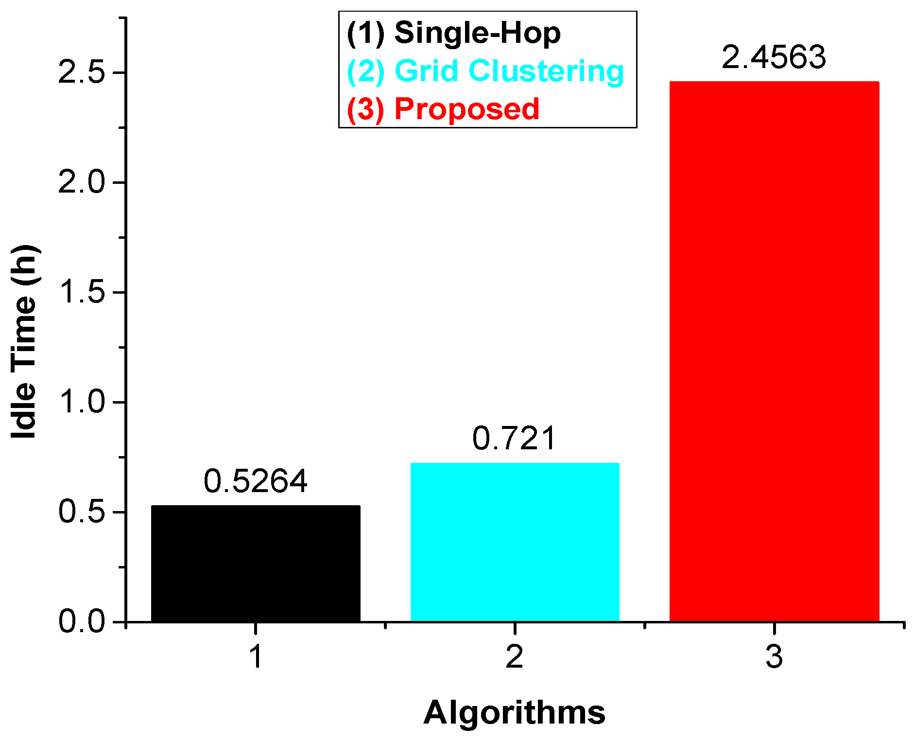
The Idle time refers to as the time spent by the wireless charging vehicle at the maintenance station. Once the charging around is accomplished, the primary objective is to maximize the idle time of the wireless charging device which plays an imperative role to augment the competence of WRSNs. However, it envisaged in Figure 4, the proposed method has increased the ratio of idle time in comparison with the literature.
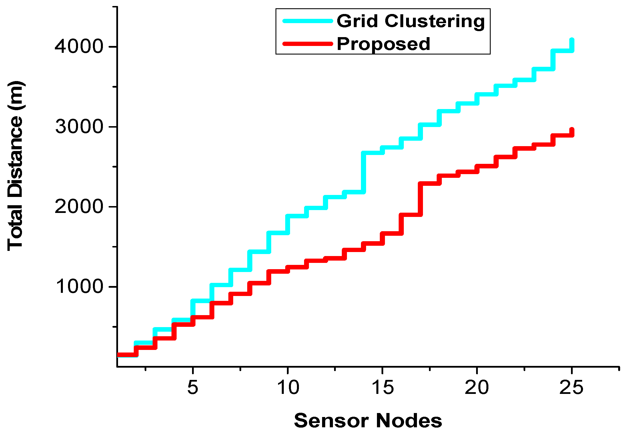
Figure 5, presents the results obtained for the total distance covered by the wireless charging device. The results illustrate that the proposed framework can reduce the total length covered by the wireless charging device.
Figure 6, shows the traveling time covered by the wireless charging device amid the existing and the proposed methodology. If a charging algorithm can charge the sensor nodes efficiently using the shortest optimal path, it may have less traveling time to replenish the sensor nodes. It has evident from the figure that the proposed algorithm is having less traveling time when compared to the benchmark algorithm.
Figure 7, shows the comparison of charging time between grid clustering and proposed algorithm. We note that the charging time of the proposed approach is shorter than that of grid clustering. The reason is that the proposed plan takes advantage of similar grouping (i.e., virtual clustering approach) along with shortest path algorithms. Furthermore, the simulation results manifested that the proposed scheme is useful in meeting the requirements of the WRSN with better network lifetime and stability period.
In the following experimental results, we essentially evaluate the charging performance of two algorithms concerning total distance, traveling time and charging time correspondingly. Nevertheless, as shown in Table 3, numerical results are given concerning total distance, travelling time and charging time.
According to Table 3, the total distance, traveling time and charging time (i.e., rechargeable cycle) of the proposed approach is less than of grid clustering. Furthermore, as a result of proposed approach pays close deliberation to location relationship along with energy awareness characteristic amid sensor nodes which results in minimizing the charging times along with charging path of the wireless charging device.
7. Conclusions
In this investigation, we have exhibited an optimization model for the problem of scheduling using a wireless charging device in the wireless rechargeable sensor network and then proposed mutually the shortest charging distance and particle swarm optimization algorithms to resolve the above issues. The virtual clustering scheme collectively used with particle swarm optimization to balance the network efficiency. We present both theoretical and practical results on the charging threshold. We evaluate the effectiveness of our proposed algorithms through extensive simulation, and experimental results have compared with the state-of-the-art algorithm. The numerical analysis evidenced that the obtained results significantly maximized the network lifetime in comparison to the existing studies. Furthermore, we will extend our work from one wireless charging device to multiple charging devices.
Author Contributions
All the authors have contributed equally to this research work.
Funding
This work was granted by Tianjin Sci-tech Planning Projects (Grant No. 14RCGFGX00846), the Natural Science Foundation of Hebei Province, China (Grant No. F2015202239).
Acknowledgments
The authors would like to show their deepest gratitude to the Hebei University of Technology for sharing their pearls of wisdom with us during the course of this research work. I gratefully acknowledge the funding received towards my doctoral study from the China Scholarship Council (CSC).
Conflicts of Interest
The authors declare no conflicts of interest.
References
- Anastasi, G.; Conti, M.; Di Francesco, M.; Passarella, A. Energy conservation in wireless sensor networks: A survey. Ad Hoc Netw. 2009, 7, 537–568. [Google Scholar] [CrossRef] [Green Version]
- Ali, A.; Ming, Y.; Chakraborty, S.; Iram, S. A comprehensive survey on real-time applications of wsn. Future Internet 2017, 9, 77. [Google Scholar] [CrossRef]
- He, S.; Chen, J.; Jiang, F.; Yau, D.K.; Xing, G.; Sun, Y. Energy provisioning in wireless rechargeable sensor networks. IEEE Trans. Mob. Comput. 2013, 12, 1931–1942. [Google Scholar] [CrossRef]
- Petrioli, C.; Spenza, D. Poster: Pro-Energy: A Novel Energy Prediction Model for Solar and Wind Energy Harvesting Wsns. In Proceedings of the 9th International Conference on Mobile Ad-Hoc and Sensor Systems (MASS 2012), Las Vegas, NV, USA, 8–11 October 2012. [Google Scholar]
- Kurs, A.; Karalis, A.; Moffatt, R.; Joannopoulos, J.D.; Fisher, P.; Soljačić, M. Wireless power transfer via strongly coupled magnetic resonances. Science 2007, 317, 83–86. [Google Scholar] [CrossRef] [PubMed]
- Fu, L.; Cheng, P.; Gu, Y.; Chen, J.; He, T. Optimal charging in wireless rechargeable sensor networks. IEEE Trans. Veh. Technol. 2016, 65, 278–291. [Google Scholar] [CrossRef]
- Xu, J.; Liu, L.; Zhang, R. Multiuser miso beamforming for simultaneous wireless information and power transfer. IEEE Trans. Signal Process. 2014, 62, 4798–4810. [Google Scholar] [CrossRef]
- Lu, X.; Wang, P.; Niyato, D.; Kim, D.I.; Han, Z. Wireless charging technologies: Fundamentals, standards, and network applications. IEEE Commun. Surv. Tutor. 2016, 18, 1413–1452. [Google Scholar] [CrossRef]
- Khaligh, A.; Zeng, P.; Zheng, C. Kinetic energy harvesting using piezoelectric and electromagnetic technologies—State of the art. IEEE Trans. Ind. Electron. 2010, 57, 850–860. [Google Scholar] [CrossRef]
- Liang, W.; Xu, W.; Ren, X.; Jia, X.; Lin, X. Maintaining large-scale rechargeable sensor networks perpetually via multiple mobile charging vehicles. ACM Trans. Sens. Netw. 2016, 12, 14. [Google Scholar] [CrossRef]
- Lu, X.; Niyato, D.; Kim, D.I.; Maso, M.; Han, Z. Wireless powered communication networks: Research directions and technological approaches. IEEE Wirel. Commun. 2017, 24, 88–97. [Google Scholar]
- Ali, A.; Ming, Y.; Si, T.; Iram, S.; Chakraborty, S. Enhancement of rwsn lifetime via firework clustering algorithm validated by ann. Information 2018, 9, 60. [Google Scholar] [CrossRef]
- Aslam, N.; Xia, K.; Haider, M.T.; Hadi, M.U. Energy-Aware Adaptive Weighted Grid Clustering Algorithm for Renewable Wireless Sensor Networks. Future Internet 2017, 9, 54. [Google Scholar] [CrossRef]
- Wang, D.; Tan, D.; Liu, L. Particle swarm optimization algorithm: An overview. Soft Comput. 2018, 22, 387–408. [Google Scholar] [CrossRef]
- Chen, Y.-C.; Jiang, J.-R. Particle swarm optimization for charger deployment in wireless rechargeable sensor networks. In Proceedings of the 2016 26th International Conference on Telecommunication Networks and Applications Conference (ITNAC), Dunedin, New Zealand, 7–9 December 2016; pp. 231–236. [Google Scholar]
- Jiang, J.-R.; Chen, Y.-C.; Lin, T.-Y. Particle swarm optimization for charger deployment in wireless rechargeable sensor networks. Int. J. Parallel Emerg. Distrib. Syst. 2018. [Google Scholar] [CrossRef]
- Lv, C.; Wang, Q.; Yan, W.; Shen, Y. Energy-balanced compressive data gathering in wireless sensor networks. J. Netw. Comput. Appl. 2016, 61, 102–114. [Google Scholar] [CrossRef]
- Tan, Y.K.; Panda, S.K. Review of Energy Harvesting Technologies for Sustainable Wsn. In Sustainable Wireless Sensor Networks; InTech: London, UK, 2010. [Google Scholar]
- Hu, C.; Wang, Y. Optimization of Charging and Data Collection in Wireless Rechargeable Sensor Networks. Int. Conf. Hum. Cent. Comput. 2016, 9567, 138–149. [Google Scholar]
- Nikoletseas, S.; Yang, Y.; Georgiadis, A. Wireless Power Transfer Algorithms, Technologies and Applications in ad hoc Communication Networks; Springer: Berlin, Germany, 2016. [Google Scholar]
- Krikidis, I.; Timotheou, S.; Nikolaou, S.; Zheng, G.; Ng, D.W.K.; Schober, R. Simultaneous wireless information and power transfer in modern communication systems. IEEE Commun. Mag. 2014, 52, 104–110. [Google Scholar] [CrossRef] [Green Version]
- PMA. Available online: http://www.powermatters.org/ (accessed on 27 August 2018).
- A4WP. Available online: http://a4wppmamerge.wwwssr6.supercp.com/ (accessed on 27 August 2018).
- WPC. Available online: http://www.wirelesspowerconsortium.com/ (accessed on 10 August 2018).
- Zhao, M.; Li, J.; Yang, Y. A framework of joint mobile energy replenishment and data gathering in wireless rechargeable sensor networks. IEEE Trans. Mob. Comput. 2014, 13, 2689–2705. [Google Scholar] [CrossRef]
- Xie, L.; Shi, Y.; Hou, Y.T.; Sherali, H.D. Making sensor networks immortal: An energy-renewal approach with wireless power transfer. IEEE/ACM Trans. Netw. 2012, 20, 1748–1761. [Google Scholar] [CrossRef]
- Peng, Y.; Li, Z.; Zhang, W.; Qiao, D. Prolonging Sensor Network Lifetime through Wireless Charging. In Proceedings of the 2010 IEEE 31st Conference on Real-Time Systems Symposium (RTSS), San Diego, CA, USA, 30 November–3 December 2010; pp. 129–139. [Google Scholar]
- Li, Z.; Peng, Y.; Zhang, W.; Qiao, D. J-roc: A joint routing and charging scheme to prolong sensor network lifetime. In Proceedings of the 2011 19th IEEE International Conference on Network Protocols, Vancouver, AB, Canada, 17–20 October 2011. [Google Scholar]
- Shi, Y.; Xie, L.; Hou, Y.T.; Sherali, H.D. On Renewable Sensor Networks with Wireless Energy Transfer. In Proceedings of the 2011 IEEE Conference on INFOCOM, Shanghai, China, 10–15 April 2011; pp. 1350–1358. [Google Scholar]
- Ren, X.; Liang, W.; Xu, W. Maximizing Charging Throughput in Rechargeable Sensor Networks. In Proceedings of the 2014 23rd International Conference on Computer Communication and Networks (ICCCN), Shanghai, China, 4–7 August 2014; pp. 1–8. [Google Scholar]
- Hu, C.; Wang, Y. Minimizing the Number of Mobile Chargers in a Large-Scale Wireless Rechargeable Sensor Network. In Proceedings of the 2015 IEEE Conference of Wireless Communications and Networking Conference (WCNC), New Orleans, LA, USA, 9–12 March 2015; pp. 1297–1302. [Google Scholar]
- Xie, L.; Shi, Y.; Hou, Y.T.; Lou, W.; Sherali, H.D. On traveling path and related problems for a mobile station in a rechargeable sensor network. In Proceedings of the 14th ACM International Symposium on Mobile Ad Hoc Networking and Computing, Bangalore, India, 29 July–1 August 2013; pp. 109–118. [Google Scholar]
- Akkaya, K.; Younis, M. An Energy-Aware Qos Routing Protocol for Wireless Sensor Networks. In Proceedings of the 23rd International Conference on Distributed Computing Systems Workshops, Providence, RL, USA, 19–22 May 2003; pp. 710–715. [Google Scholar]
- Wang, G.; Cao, G.; La Porta, T.; Zhang, W. Sensor Relocation in Mobile Sensor Networks, INFOCOM 2005. In Proceedings of the 24th Annual Joint Conference of the IEEE Computer and Communications Societies, Miami, FL, USA, 13–17 March 2005; pp. 2302–2312. [Google Scholar]
Figure 1.
A wireless rechargeable sensor network (WRSN) structural model based on clustering via single-hop & multiple-hop.
Figure 1.
A wireless rechargeable sensor network (WRSN) structural model based on clustering via single-hop & multiple-hop.

Figure 2.
WRSN data flow diagram.

Figure 3.
Energy consumption of different schemes.

Figure 4.
Idle time of difference schemes.

Figure 5.
Comparison of total distance.

Figure 6.
Comparison of traveling time.

Figure 7.
Comparison of charging time.


Table 1.
The notations used.
| Notation | Definition |
|---|---|
| WCD | Wireless charging device |
| N | Sensor nodes (SNs) |
| BS | Base Station node |
| MS | Maintenance Station |
| The maximum battery capacity of sensor nodes | |
| The minimum energy required to SNs work properly | |
| Traveling speed of the wireless charging device | |
| The full charging power | |
| The data rate generates in the network at SN | |
| Communication radius | |
| The data flow rate in the network from SN to SN at the time | |
| The energy consumption coefficient for receiving the data | |
| The energy consumption for forwarding the data from SN to SN | |
| The rate of energy consumption from SN to SN at the time | |
| The time an SN in the network performs a charging task | |
| WCD spends the time to charge sensor node | |
| The wireless charging device at the service station for vacation | |
| The centroid | |
| xi, yi | The coordinates of SN |
| The time interval between centroid and sensor node | |
| Indicates the completion of one round of transmission cycle in WRSN |
Table 2.
Simulation Setting.
| Parameters | Values |
|---|---|
| Network Size | 1000 m × 1000 m |
| Number of Nodes () | 25 |
| Initial energy ) | 10,800 J |
| Minimal energy ) | 540 J |
| Moving Speed | 5 m/S |
| Charging Power | 5 W |
| Communication radius (Rc) | 100 m |
| Path Loss | Log-Normal Shadowing |
| Antenna | Omni Directional |
| Charging Scheme | Grid Clustering, particle swarm optimization algorithm (PSO) |
| Simulation Period | 1 h |
Table 3.
Charging Performance.
| Properties Values | |||||||||
|---|---|---|---|---|---|---|---|---|---|
| Total Distance (m) | Traveling Time (s) | Charging Time (s) | |||||||
| Algorithms | 10 | 25 | 50 | 10 | 25 | 50 | 10 | 25 | 50 |
| Grid Clustering | 1884 | 4089 | 6763 | 376 | 817 | 1353 | 386 | 842 | 1395 |
| Proposed | 1245 | 2968 | 6142 | 249 | 593 | 1228 | 259 | 618 | 1277 |
© 2018 by the authors. Licensee MDPI, Basel, Switzerland. This article is an open access article distributed under the terms and conditions of the Creative Commons Attribution (CC BY) license (http://creativecommons.org/licenses/by/4.0/).
Share and Cite
MDPI and ACS Style
Ali, A.; Ming, Y.; Chakraborty, S.; Iram, S.; Si, T. The Augmented Approach towards Equilibrated Nexus Era into the Wireless Rechargeable Sensor Network. Symmetry 2018, 10, 639. https://0-doi-org.brum.beds.ac.uk/10.3390/sym10110639
AMA Style
Ali A, Ming Y, Chakraborty S, Iram S, Si T. The Augmented Approach towards Equilibrated Nexus Era into the Wireless Rechargeable Sensor Network. Symmetry. 2018; 10(11):639. https://0-doi-org.brum.beds.ac.uk/10.3390/sym10110639
Chicago/Turabian StyleAli, Ahmad, Yu Ming, Sagnik Chakraborty, Saima Iram, and Tapas Si. 2018. "The Augmented Approach towards Equilibrated Nexus Era into the Wireless Rechargeable Sensor Network" Symmetry 10, no. 11: 639. https://0-doi-org.brum.beds.ac.uk/10.3390/sym10110639
Note that from the first issue of 2016, this journal uses article numbers instead of page numbers. See further details here.