Dynamics of Trapped Solitary Waves for the Forced KdV Equation


Department of Applied Mathematics, Kyunghee University, Yongin-si, Korea
Symmetry 2018, 10(5), 129; https://0-doi-org.brum.beds.ac.uk/10.3390/sym10050129
Submission received: 27 March 2018
/
Revised: 22 April 2018
/
Accepted: 23 April 2018
/
Published: 24 April 2018
(This article belongs to the Special Issue Symmetry and Complexity)
Abstract
:The forced Korteweg-de Vries equation is considered to investigate the impact of bottom configurations on the free surface waves in a two-dimensional channel flow. In the study of shallow water waves, the bottom topography plays a critical role, which can determine the characteristics of wave motions significantly. The interplay between solitary waves and the bottom topography can exhibit more interesting dynamics of the free surface waves when the bottom configuration is more complex. In the presence of two bumps, there are multiple trapped solitary wave solutions, which remain stable between two bumps up to a finite time when they evolve in time. In this work, various stationary trapped wave solutions of the forced KdV equation are explored as the bump sizes and the distance between two bumps are varied. Moreover, the semi-implicit finite difference method is employed to study their time evolutions in the presence of two-bump configurations. Our numerical results show that the interplay between trapped solitary waves and two bumps is the key determinant which influences the time evolution of those wave solutions. The trapped solitary waves tend to remain between two bumps for a longer time period as the distance between two bumps increases. Interestingly, there exists a nontrivial relationship between the bump size and the time until trapped solitary waves remain stable between two bumps.
1. Introduction
Free surface waves of a two-dimensional channel flow for an inviscid and incompressible fluid have been studied when the rigid bottom of the channel has some obstacles [1,2]. Such free surface waves of shallow water with obstacles can be modeled by the forced Korteweg-de Vries (fKdV) equations [3,4]. There have been enormous applications of the Korteweg-de Vries (KdV) equation in various research areas such as mathematics, physics, fluid mechanics and hydrodynamics. The KdV equation with a forcing approximately describes the evolution of the free surface when a fluid flows over an obstacle. This forced KdV equation is related to the physical problems such as shallow-water waves over rocks, tsunami waves over obstacles, oceanic stratified flows encountering topographic obstacles, and acoustic waves on a crystal lattice. Moreover, it can be useful for other nonlinear differential equations including a nonlinear Schrodinger equation and a sine Gordon equation. These applications range from magnetohydrodynamic waves, geostrophic turbulence, atmosphere dynamics and the propagation of short laser pulses in optical fibers (see [5,6] and references therein).
The dynamics of the free surface wave motions is characterized by the Froude number F defined as , where C is the upstream velocity and is the critical speed of a shallow water wave with the finite depth of the channel h and the gravity constant g. It can be expressed as with the perturbation measurement to the critical value 1 for a positive small parameter , then the forced Korteweg-de Vries (fKdV) equation can be obtained. Further, the flow can be classified as supercritical if and subcritical if . For supercritical flows, there is a critical value, , such that solitary wave solutions exist when and no such solutions exist when . Solitary wave solutions present some special features such as remaining stable without any changes in shape or speed when they evolve in time. Moreover, this critical value of is dependent on the bump configuration.
The bottom topography is a key determinant for the characteristic of wave motions. Interesting surface wave phenomena can be observed when a bottom topography is rather complicated. For one bump, there has been extensive analytic and numerical work [1,3,7,8]. Cusped stationary solitary wave solutions are founded analytically and their numerical stability is shown for the Dirac delta function as forcing [9]. It is well known that there exist two branches of stationary solitary wave solutions when a semi-circular bump is given [10]. One is the near zero solitary wave with lower amplitude and the other one is a higher amplitude one -shaped wave). Analytic stability of solitary wave solutions is discussed for the time-dependent forced KdV equation when a compactly supported symmetric bump is given [7]. It is proved that the near zero solution is stable with respect to time for a sufficiently large . The other solitary wave solution -shaped solution) is unstable when it evolves in time.
Recently, more researchers pay attention to the cases where bottom configurations are more complicated [11,12]. For subcritical flows, the generalized hydraulic falls have been obtained when two bumps are given [13]. These solutions are characterized by a train of waves ‘trapped’ between two bumps satisfying the radiation conditions at the infinity. The steady surface flows over a step and a rectangular obstacle have been investigated for supercritical, subcritical waves and hydraulic falls [14]. Various stationary solutions are explored when the bottom configurations are complex including one positive bump, one negative hole, or combinations of both [15]. Stationary solutions of the forced KdV with obstacles with a negative hole have been illustrated as the amplitude and the width of a negative hole are varied [16].
Analytic and numeric stationary solutions of the forced KdV equations are studied when one bump or two bumps are given as forcing, which are in the form of - or -functions [17]. They also explored the stability of solitary waves and table-top solutions when they evolve in time. Multiple stationary supercritical solutions of the fKdV equation are discussed when two-semi-circular bumps are given [18]. Their results show that there exists only one supercritical positive solitary wave, which is stable when it evolves in time. Solitary wave solutions and their time evolutions are investigated when the rigid bottom has one negative hole [19,20]. Interestingly, there are five stationary solutions when a negative hole is given and only the near zero wave remains stable when they evolve in time [19].
In our previous study, stationary trapped solitary wave solutions have been studied for the forced Korteweg-de Vries equation when two bumps or two holes are given as the bottom configuration [21]. Some of multiple stationary solitary waves have been found and then their numerical stability has been investigated in the presence of two bumps [22]. Interestingly, multiple trapped supercritical wave solutions remain stable between two bumps for a very long time when they evolve in time. It is worth noting that the interplay between trapped solitary waves and two bumps plays a key role in determining their time evolutions. In this work, we extend the previous work by exploring the impact of different two-bump scenarios on the trapped solitary waves and their numerical stability. First, various stationary trapped solitary wave solutions of the forced KdV equation have been obtained in the presence of two bumps or two holes. As the bump size or the distance between two bumps are varied, stationary solitary waves are obtained. Next, we employ the semi-implicit finite difference method which has been developed for the homogeneous KdV equation [23]. This numerical method has been used to obtain the time evolution of the trapped stationary solitary waves. Our numerical results show that multiple trapped solitary wave solutions stay stable between two bumps for a very long time under various two-bump configurations. This indicates that the interplay between trapped solitary waves and two bumps highlights the importance in determining the dynamics of trapped solitary waves.
2. The Forced KdV Equation
2.1. Model Equation with Two-Bump Configurations
The forced KdV equation is written as follows
where is the free surface elevation measured from an undisturbed water level, and is the measurement of the perturbation of the upstream uniform flow velocity from its critical value. The external forcing is given by the topography of the rigid bottom. Our main interests in this work are numerical stability when stationary wave solutions evolve in time. Hence, the problem (1) defined in can be restricted to a finite interval for a positive constant b, where this interval is large enough to use a finite difference scheme. First, at these finite boundaries, we employ the artificial boundary condition, which has been proposed in [21]. Then, the time-independent nonlinear boundary value problem is efficiently solved using the Newton method with the artificial boundary condition which is described as
As shown in [21], the method provides a good alternative to find various stationary solutions under arbitrary two-bump configurations. Once the stationary wave solutions have been found, we take these stationary solutions as initial conditions in (1). Next, the finite difference method described in the next subsection is performed to solve the time-dependent forced KdV equation in a finite interval for .
Moreover, the bottom topography is modeled by the following functions for two bumps
Note that consists of two bumps (centered at a and ) with the distance between the boundaries of two bumps, .
2.2. Semi-Implicit Finite Difference Method
The problem (1) defined in can be restricted to a finite interval for a positive constant b. This Initial Boundary Value Problem has a third order derivative with respect to x and, due to the presence of a forcing, the direction of wave propagation is unknown. Therefore, it is not a trivial task to impose the correct boundary conditions at finite boundaries. This leads us to solve the alternative form of the forced KdV equation. This results in the following Initial Boundary Value problem
The problem involves the fourth derivative for the spatial variable, therefore four boundary conditions are required. This is done by imposing the zero Neumann boundary conditions at each boundary. Now, we employ the finite difference scheme to find the numerical solutions of equation above. Let us denote , , and where and with positive integers N and , respectively. First, the Crank-Nicolson scheme with standard difference schemes is applied to (3) and the resulting finite difference equations are written as
for , . The standard finite difference is used for forward , backward , central , , and .
Note that the nonlinear term is linearized by taking a Taylor expansion for the nonlinear convection term as
where . Therefore, the nonlinear convection term can be linearized in the following form
Substituting (6) into (4) leads to the following system
where
and
where , . This system is solved at each time step. The computational domain is taken to be b= 50 with and . Our scheme is based on the linearized implicit scheme as proposed in [23,24]. This scheme is unconditionally linearly stable with a local truncation error, . Therefore, there is no restriction on and (more details on this numerical scheme are found in [23,24]).
3. Numerical Simulations
In this section, we present numerical simulations under various two-bump configurations including two bumps (positive forcing) or two holes (negative forcing). Our main focus is on trapped solitary waves between two bumps or two holes and their stability as they evolve in time. In particular, the bottom configuration is confined as two identical or symmetric positive bumps or negative holes. First, stationary trapped solitary waves are found as varying the distance between two bumps and the bump size. Then, we investigate the impact of various bump scenarios on their numerical stability.
3.1. Trapped Solitary Waves between Two Positive Bumps
As well known, the time independent KdV equation without any forcing (i.e. ) has two exact solutions such as and with a phase shift . Also, in the presence of a single positive symmetric forcing which satisfies a compact support condition, there are two symmetric solitary wave solutions: one is near and the other one is near for all with a critical value [7]. Under two-bump configurations, with the similar argument, there exist at least two stationary solitary wave solutions, since the bump is positive and symmetric with a compact support. Recall that is defined as each bump is centered at and a and the bump height at each center is .
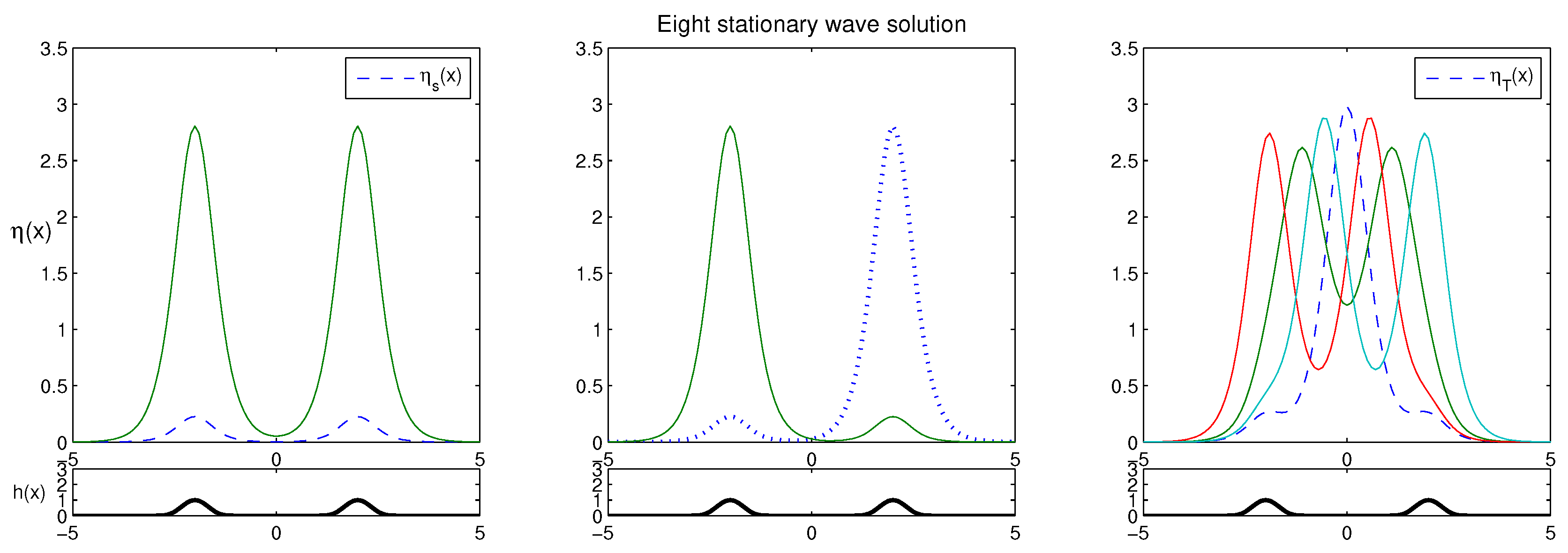
Figure 1 displays eight stationary wave solutions using the two-bump configuration and . The left panel shows two symmetric solitary wave solutions including the lower amplitude wave (blue dashed), which is the near zero solution denoted by . Two non-symmetric wave solutions (with lower and higher amplitude, respectively) are shown in the middle panel. The right panel represents four stationary wave solutions which consist of two symmetric solutions and two non-symmetric ones. The blue dashed wave illustrated in the right panel of Figure 1 depicts the solitary wave solution which is trapped between two bumps similar to (-type wave is placed in the middle of two bumps). Let this be referred to as a trapped solitary wave solution and denoted by . In this study, we focus on the dynamics of these trapped solitary waves, (a higher amplitude wave in the middle of two bumps) under various bump configurations.
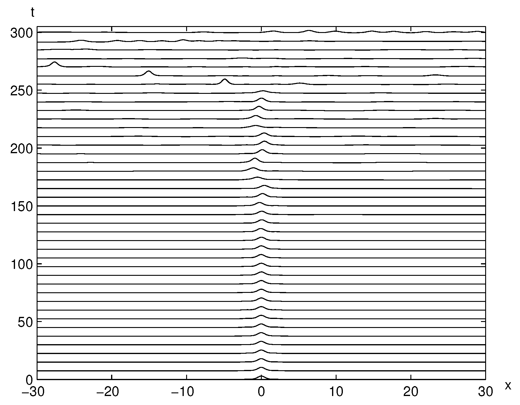
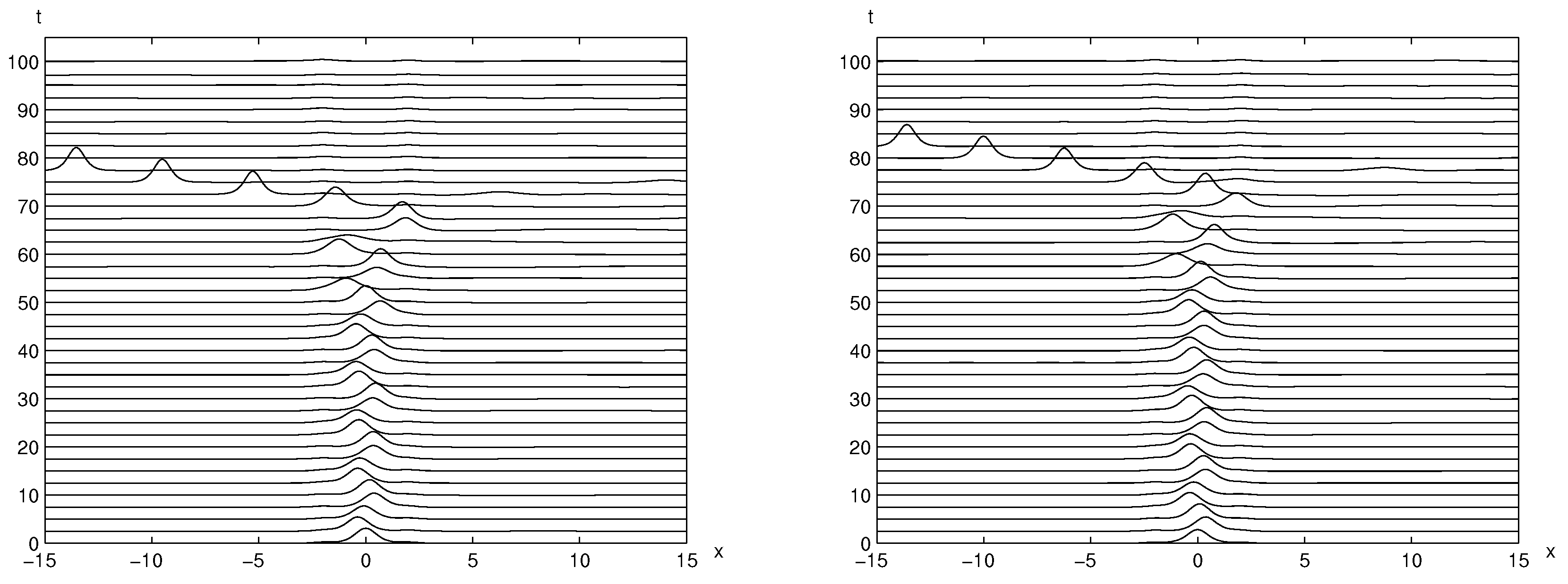
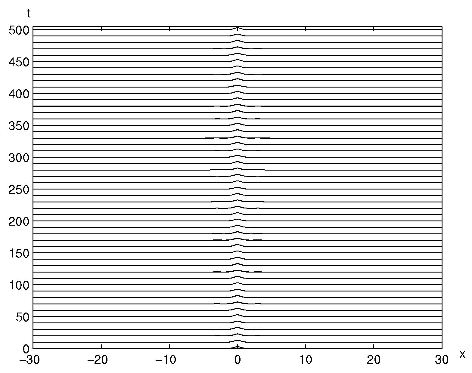
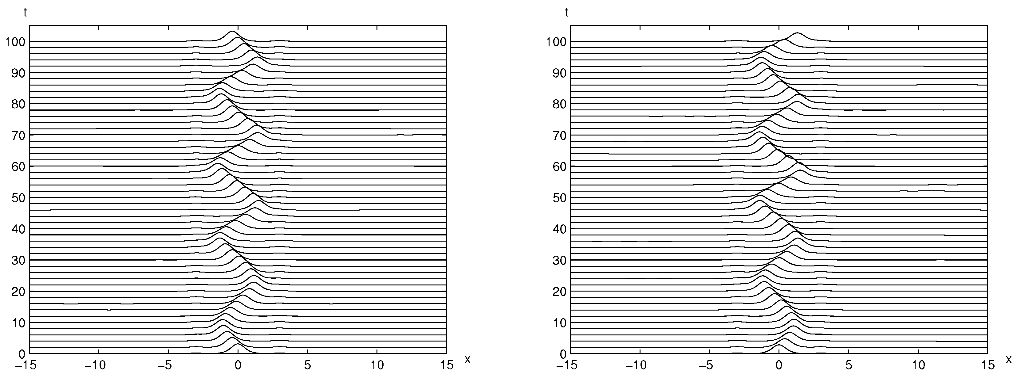
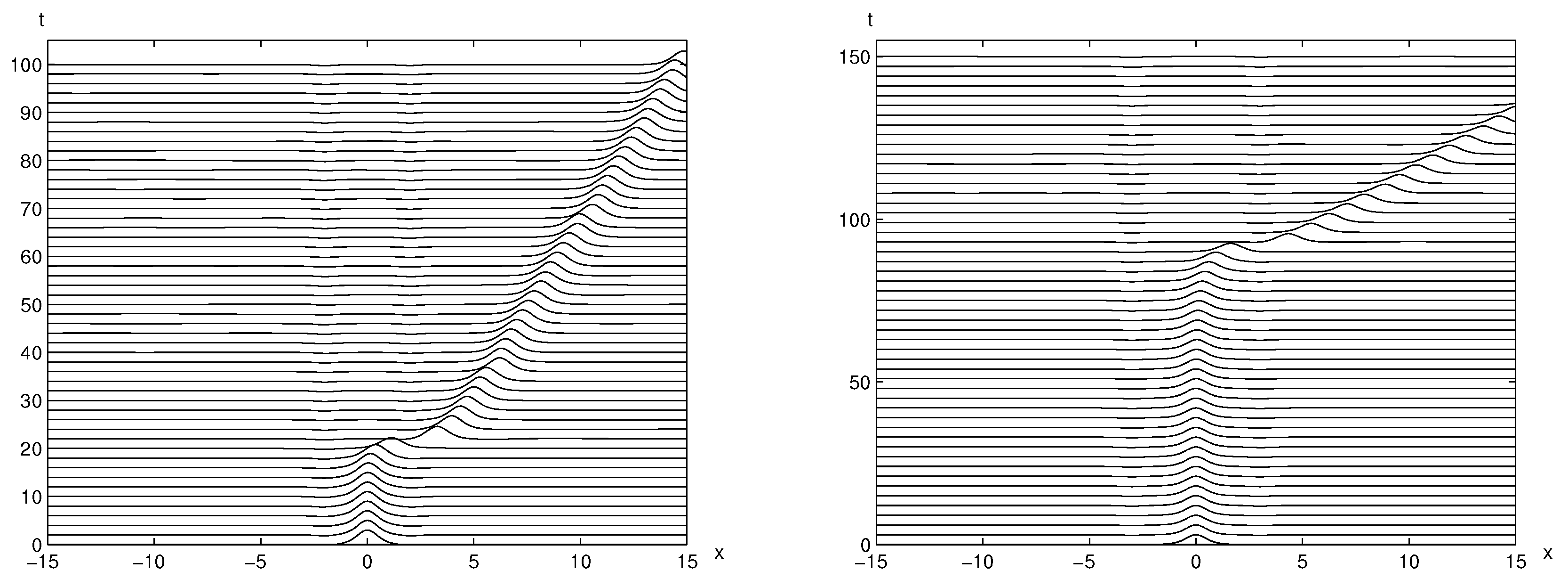
It is well known that the near zero wave solution is stable with respect to time when either single positive symmetric bump or two positive bumps is given. The solitary wave solutions with two higher amplitudes (the solid curves in the left panel of Figure 1) are moving out fast since they are placed right over the bumps and this makes them unstable in a very short time. However, the trapped solitary wave which is placed between two bumps ( in the right panel of Figure 1) remains stable for a very long time as observed [22]. Here, the time evolution of the trapped solitary wave, is revisited in Figure 2 and Figure 3. The unperturbed trapped solitary wave solution () remains stable between two bumps until in Figure 2. Figure 3 displays the time evolutions of perturbed trapped solitary wave solutions with and perturbation, respectively. Under perturbations, trapped solitary waves start moving out of two bumps around . It is worth noting that the trapped solitary wave consists of the unforced solitary wave and the near zero solitary waves with two bumps. Hence, we can conjecture that the trapped solitary wave remains stable up to a certain time due to the stable interplay between and .
3.2. The Impact of the Bump Distance on the Stability of
We investigate the impact of the distance between two bumps on the trapped solitary waves. Figure 4 illustrates three stationary trapped solitary wave solutions using three different bump distances between two bumps. All of their shapes are similar to around with the near zero wave just over each bump. The distance between two bumps are varied as 2, 4 and 6 using , and , respectively. Their time evolutions are illustrated in Figure 5 and Figure 6.
First, the time evolution of the unperturbed trapped solitary wave solution is displayed using (the distance between two bumps is 4) in Figure 5. It is interesting to observe that the trapped solitary wave solution is stable up to a very long time (simulated until ). This can be compared with the unperturbed result with stable up to in Figure 2. Next, the trapped solitary wave using are perturbed with and in Figure 6. They move back and forth between two bumps, however, they still remain between two bumps for a very long time (the results shown until ).
3.3. The Impact of the Bump Size on the Stability of
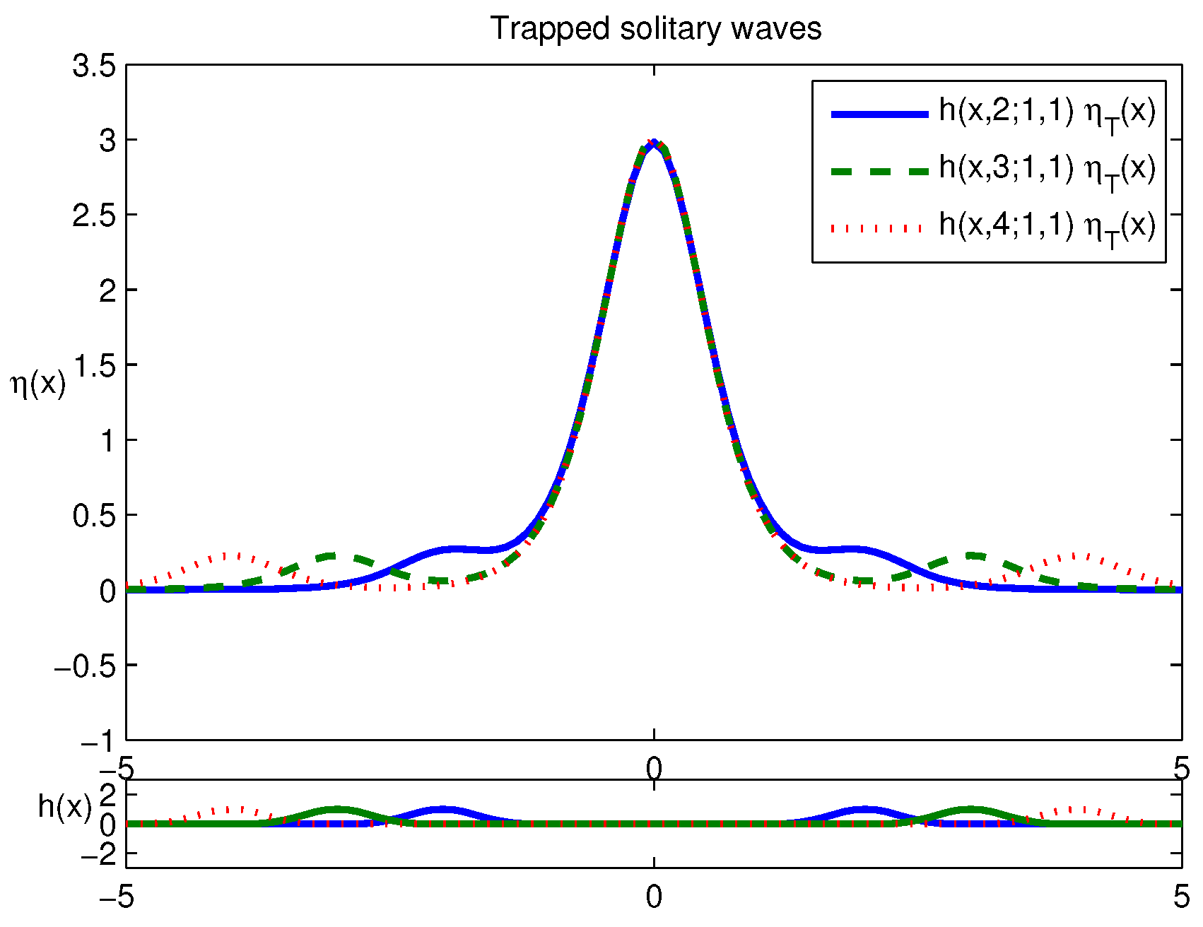
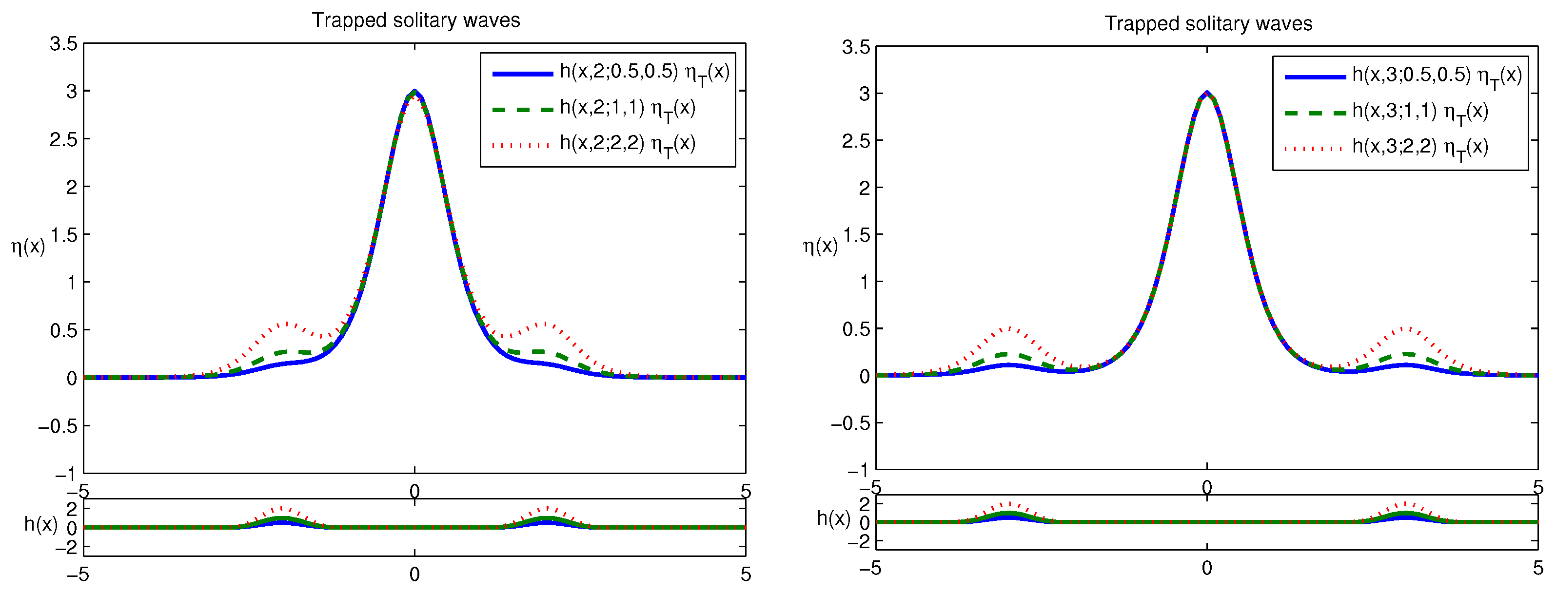
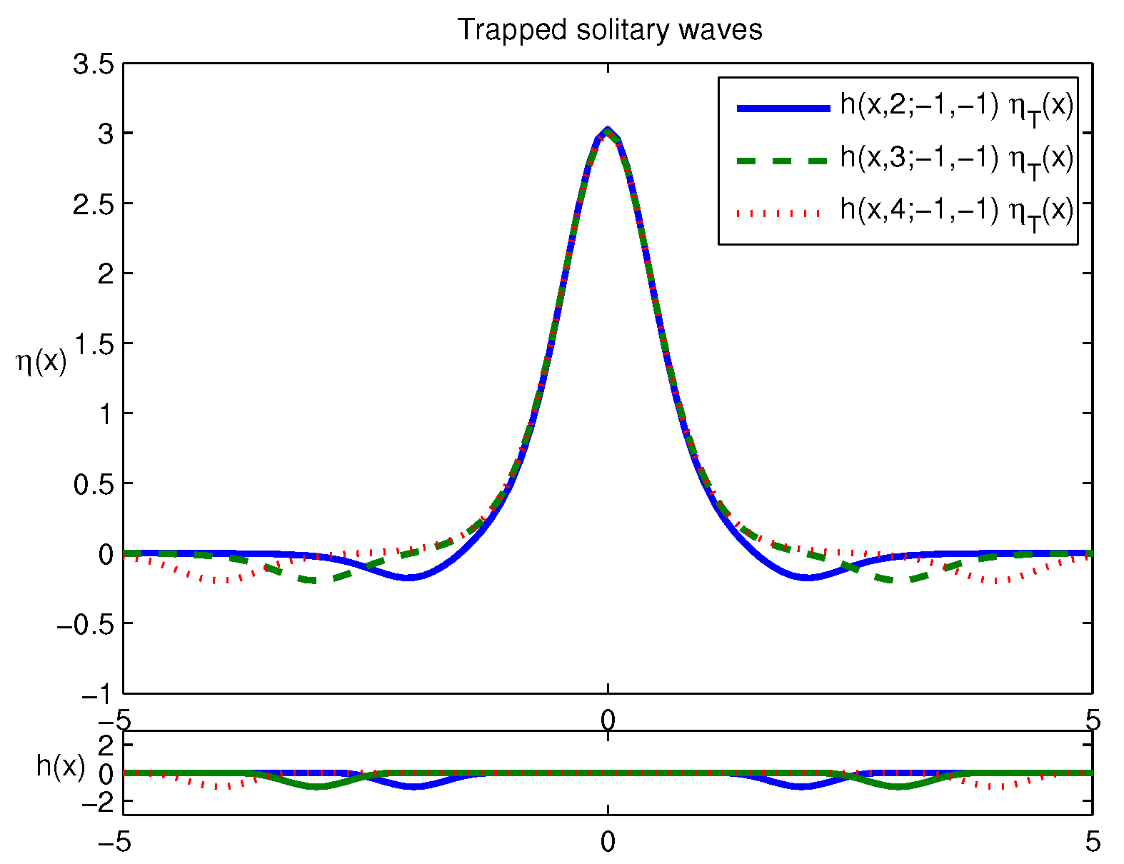
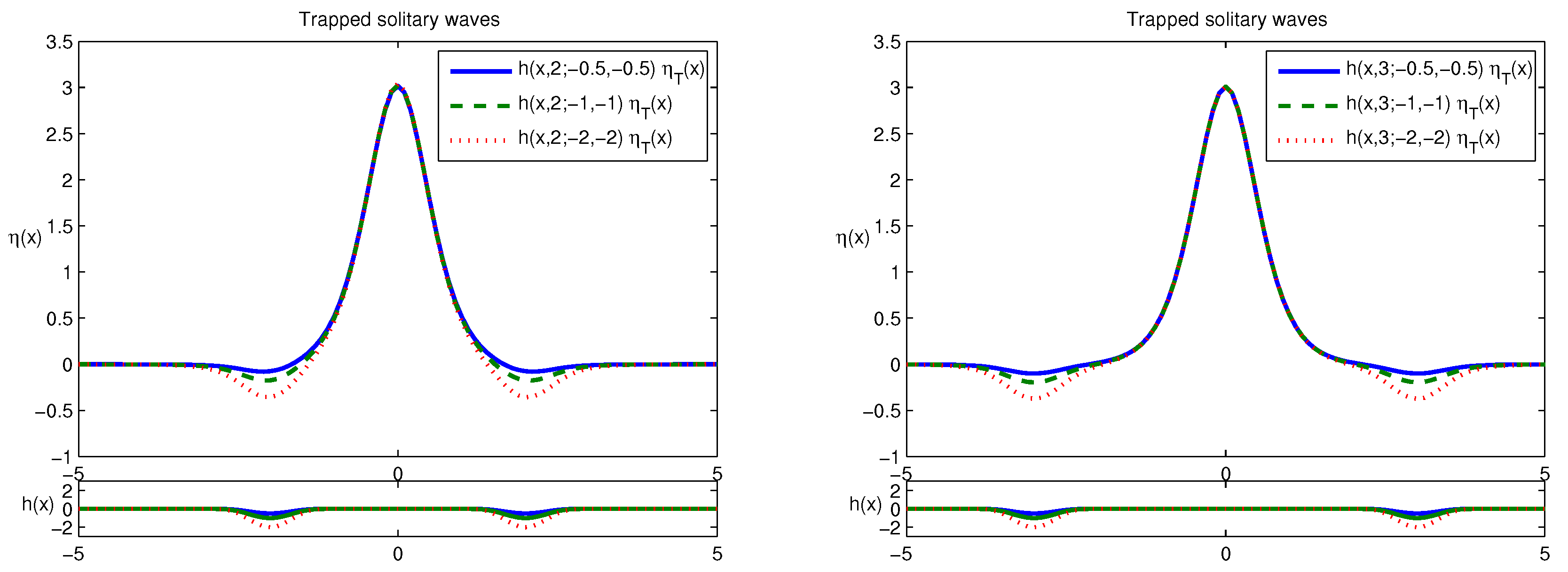
The impact of the size of two bumps on the time evolutions for trapped solitary waves has been explored. Let us consider our baseline bump size to be 1 (the bump size is defined as the maximum height of the bump at the center, which is ). Now, the bump size is varied from to 2. As shown in Figure 7, each stationary trapped solitary wave has the shape of around and the near zero wave over each bump. Also, the distance between two bumps is varied as well; the left panel shows the result with the bump distance 2 and the right panel with the bump distance 4. The amplitude of near zero wave gets higher as the bump size becomes larger in both panels.
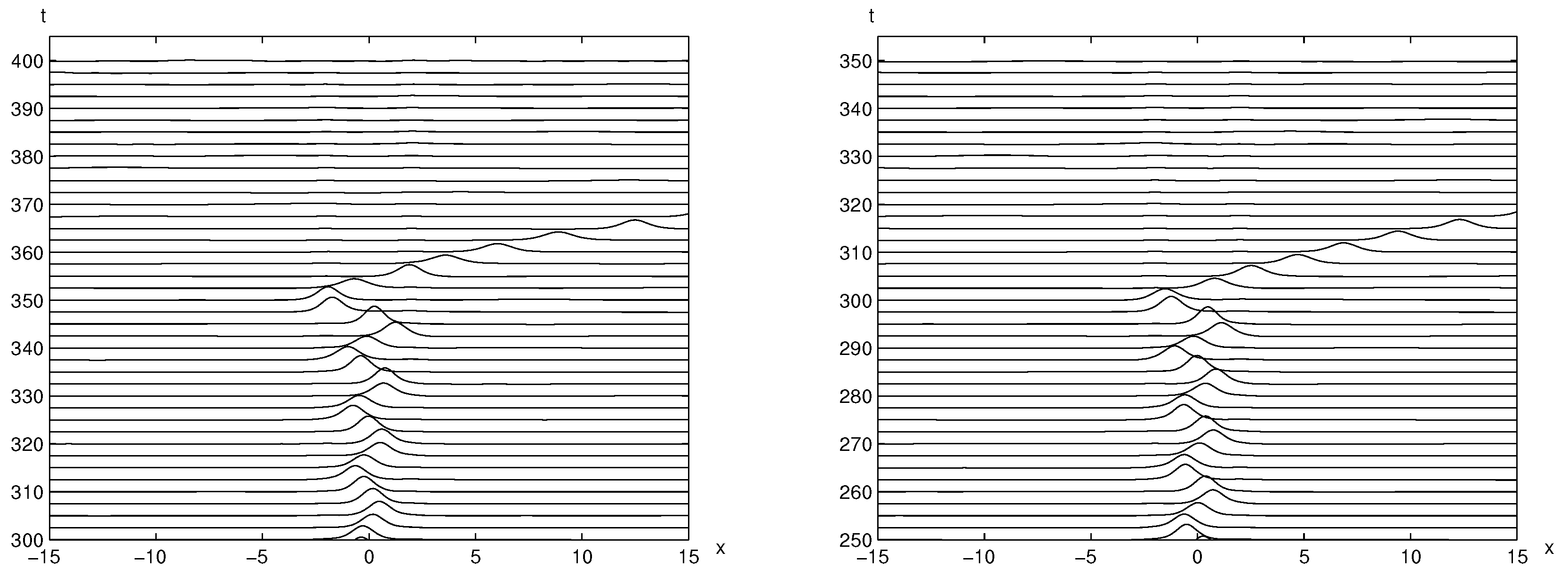
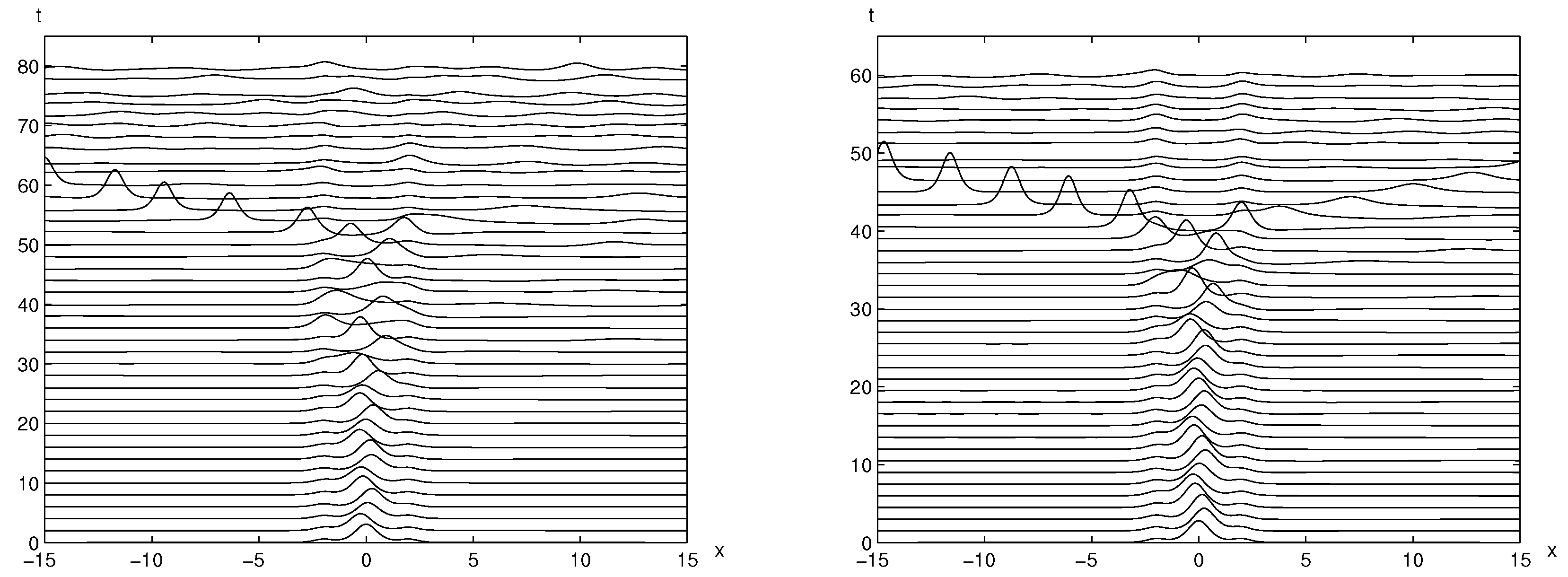
The time evolutions of the perturbed trapped solitary wave solution using with and are displayed in Figure 8. Note that the perturbed trapped solitary wave solution stays much longer between two bumps when comparing with the results in Figure 4. That implies that the trapped solitary wave with the bump size is more stable than the ones with the bump size 1. Now, using the larger bump size, Figure 9 illustrates that the perturbed trapped solitary wave solutions with the bump size 2 moves out of two bumps quickly than the results in Figure 4. This indicates that there is a critical bump size for trapped solitary waves to remain stable for a longer time. Therefore, we investigate the relationship between the bump size and the time until trapped solitary waves remain stable.
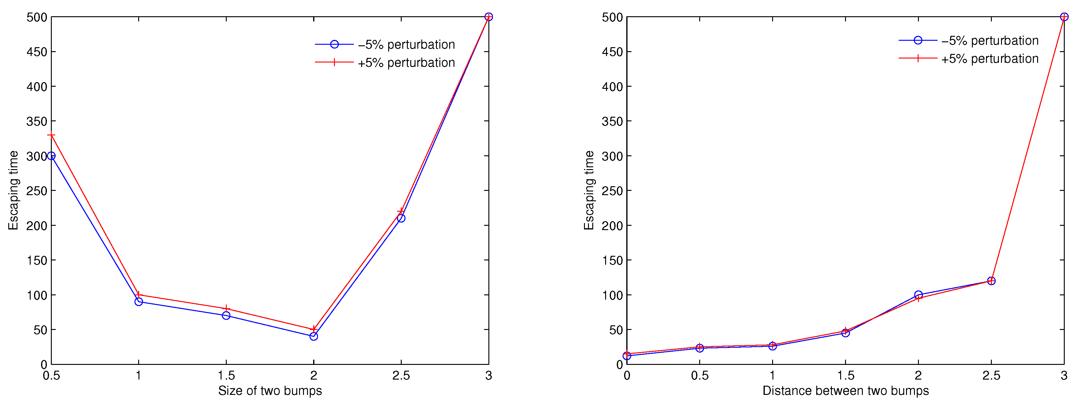
The left panel of Figure 10 displays the time when the trapped solitary wave solutions move out of two bumps as the bump size is varied. The time is measured when trapped solitary waves under (solid) or (dotted) perturbation start moving out of two bumps. The time decreases when the bump size increases from 0.5 to 2 so that it takes the minimum around the bump size 2, then the time increases again significantly as the bump size increases. Next, we investigate the relationship between the bump distance and the time until trapped solitary waves remain stable. The right panel of Figure 10 illustrates the time when the trapped solitary wave solutions move out of two bumps as the bump distance is varied. Again, the time is measured when trapped solitary waves under (solid) or (dotted) perturbation start moving out of two bumps. As seen in the right panel, the time increases as the distance between two bumps increases linearly.
3.4. Trapped Solitary Waves between Two Negative Holes
In this subsection, we present the dynamics of trapped solitary waves when two negative holes are given as the bottom configuration. As studied in [19], there are five stationary wave solutions including the near zero wave (a negative solitary wave) and the near wave in the presence of one negative bump or hole. Unlike the solitary wave of a positive bump, the near zero solitary wave exists for all when a negative bump is given. Moreover, the near zero wave is stable and the near wave is unstable when they evolve in time [19]. In the presence of two symmetric negative holes, the number of stationary solitary wave solutions increase (the larger the distance between two holes, the more various trapped solitary waves [21]).
First, stationary trapped solitary wave solutions between two holes are obtained as the distance between two holes is varied. In Figure 11, three stationary trapped solitary wave solutions are displayed under three different bump distance using , and , respectively. Each trapped solitary wave has the shape of around and the near zero negative wave over each hole. Next, Figure 12 illustrates stationary trapped solitary waves as the hole depth is varied, , and . Further, the left panel of Figure 12 shows the trapped solitary waves using the hole distance 2 and the right panel shows the trapped solitary waves using the hole distance 4.
Figure 13 and Figure 14 illustrate the time evolutions of unperturbed trapped solitary wave solutions. As seen in both figures, the trapped solitary waves move out of two holes much faster than the cases of two symmetric positive bumps. In Figure 13, the trapped solitary wave stays between two holes up to with (right) while it stays only up to with (left). This is consistent with the results for two positive bumps; the larger the distance between two holes, the longer the trapped solitary wave solution remains stable between two holes. Similarly, as we vary the depth of two holes, the time evolutions of trapped solitary waves are changing as well in a complex way. As the depth of two holes is reduced half , the trapped solitary wave remains between two holes for a longer time (see the left panel of Figure 14). The depth of two holes is increased double , the trapped solitary wave remains between two holes for a shorter time (see the right panel of Figure 14). Again, this is consistent with the results for two positive bumps.
4. Conclusions
In this work, the focus has been on the trapped solitary wave solutions of the forced KdV and their numerical stability in the presence of two bumps. We use the Newton method incorporating artificial boundary conditions to find various trapped solitary waves in the presence of two positive bumps and two negative holes. This method provides a good alternative to find various stationary wave solutions under arbitrary two-bump configurations when they are close enough (the distance between two bumps are not large) [21]. The semi-implicit finite difference method has been employed to investigate the numerical stability of these trapped solitary waves. Our previous results indicate that the number of stationary wave solutions increases as the bump distance increases and there exist multiple trapped solitary waves under different two-bump configurations [22]. In this study, we have extended the results under more various two bump configurations. Specifically, the impact of the bump distance and the bump size on numerical stability of trapped solitary waves have been investigated.
For both two positive bumps and two negative holes, the near zero solution is stable when it evolves in time. Moreover, it is worth to observe that a trapped wave solution remains stable for a very longer time between two positive bumps. As the distance between two bumps increases, trapped solitary waves stay longer in a straightforward fashion. On the other hand, the relationship for the bump size and the time trapped solitary waves to remain between the bumps is not trivial. There is a critical bump size for the trapped solitary to be stable for a longer time. Furthermore, for two negative holes, the trapped solitary waves do not remain for a long time as two positive bumps are given. Their time evolutions are characterized by the interplay between trapped solitary waves and two-bump configurations.
However, for non-symmetric bumps (two bumps or two holes with different sizes), trapped solitary waves become non-symmetric as well and they move out of two bumps in a much shorter time. Non-symmetry becomes even more significant in stationary solitary waves for the combined bottom configuration of a bump and a hole. They lose stability too fast to measure the length of time where solitary waves are stable. This highlights the importance of symmetry in the bumps and solitary waves for their stability. We find that the interplay between trapped solitary waves and two bumps becomes stronger so that they remain stable up to a certain time when two positive bumps are given. Hence, we can conjecture that two positive bumps provide a trap for some trapped wave solutions to be stable for a certain finite time.
Acknowledgments
This work was supported by the National Research Foundation of Korea (NRF) grant funded by the Korean government (MSIP) (NRF-2015R1C1A2A01054944).
Conflicts of Interest
The authors declare no conflict of interest.
Abbreviations
The following abbreviations are used in this manuscript:
| MDPI | Multidisciplinary Digital Publishing Institute |
| DOAJ | Directory of open access journals |
| TLA | Three letter acronym |
| LD | linear dichroism |
References
- Camassa, R.; Wu, T. Stability of forced solitary waves. Philos. Trans. R. Soc. Lond. A 1991, 337, 429–466. [Google Scholar] [CrossRef]
- Zabuski, N.J.; Kruskal, M.D. Interaction of “solitons” in a collisionless plasma and the recurrence of initial states. Phys. Rev. Lett. 1965, 15, 240–243. [Google Scholar] [CrossRef]
- Dias, F.; Vanden-Broeck, J.M. Generalized critical free-surface flows. J. Eng. Math. 2002, 42, 291–301. [Google Scholar] [CrossRef]
- Shen, S.S. On the accuracy of the stationary forced Korteweg-De Vries equation as a model equation for flows over a bump. Q. Appl. Math. 1995, 53, 701–719. [Google Scholar] [CrossRef]
- Crighton, D.G. Applications of KdV. Acta Appl. Math. 1995, 39, 39–67. [Google Scholar] [CrossRef]
- Hereman, W. Shallow Water Waves and Solitary Waves. In Mathematics of Complexity and Dynamical Systems; Meyers, R., Ed.; Springer: New York, NY, USA, 2012. [Google Scholar]
- Choi, J.W.; Sun, S.M.; Whang, S.I. Supercritical surface gravity waves generated by a positive forcing. Eur. J. Mech. B Fluids 2008, 27, 750–770. [Google Scholar] [CrossRef]
- Shen, S.S.; Shen, M.C.; Sun, S.M. A model equation for steady surface waves over a bump. J. Eng. Math. 1989, 23, 315–323. [Google Scholar] [CrossRef]
- Shen, S.S.; Manohar, R.P.; Gong, L. Stability of the lower cusped solitary waves. Phys. Fluids 1995, 7, 2507–2509. [Google Scholar] [CrossRef]
- Forbes, L.K. Critical free-surface flow over a semi-circular obstruction. J. Eng. Math. 1988, 22, 3–13. [Google Scholar] [CrossRef]
- Grimshaw, R.; Maleewong, M. Stability of steady gravity waves generated by a moving localised pressure disturbance in water of finite depth. Phys. Fluids 2013, 25, 006705. [Google Scholar] [CrossRef]
- Pratt, L.J. On nonlinear flow with multiple obstructions. Geophys. Astrphys. Fluid Dyn. 1984, 41, 1214–1225. [Google Scholar] [CrossRef]
- Dias, F.; Vanden-Broeck, J.M. Trapped waves between submerged obstacles. J. Fluid Mech. 2004, 509, 93–102. [Google Scholar] [CrossRef]
- Binder, B.J.; Dias, F.; Vanden-Broeck, J.M. Influence of rapid changes in a channel bottom on free-surface flows. IMA J. Appl. Math. 2008, 73, 254–273. [Google Scholar] [CrossRef]
- Binder, B.J.; Blyth, M.G.; McCue, S.W. Free-surface flow past arbitrary topography and an inverse approach for wave-free solutions. IMA J. Appl. Math. 2013, 78, 685–696. [Google Scholar] [CrossRef]
- Ee, B.K.; Grimshaw, R.H.J.; Zang, D.H.; Chow, K.W. Steady transcritical flow over a hole: Parametric map of solutions of the forced Korteweg-de Vries equation. Phys. Fluids 2010, 22, 056602. [Google Scholar] [CrossRef]
- Chardard, F.; Dias, F.; Nguyen, H.Y.; Vanden-Broeck, J.M. Stability of some stationary solutions to the forced KdV equation with one or two bumps. J. Eng. Math. 2011, 70, 175–189. [Google Scholar] [CrossRef]
- Gong, L.; Shen, S.S. Multiple wave solutions of the staionary forced Korteweg-De Vries equation and their stability. SIAM J. Appl. Math. 1994, 54, 1268–1290. [Google Scholar] [CrossRef]
- Choi, J.W.; Lin, T.; Sun, S.M.; Whang, S.I. Supercritical surface waves generated by negative or oscillatory forcing. Discret. Contin. Dyn. Syst. B 2010, 14, 1313–1335. [Google Scholar] [CrossRef]
- Choi, J.W. Free surface waves over a depression. Bull. Aust. Math. Soc. 2002, 65, 329–335. [Google Scholar] [CrossRef]
- Whang, S.I.; Lee, S.M. Absorbing boundary conditions for the stationary forced KdV equation. Appl. Math. Comput. 2008, 202, 511–519. [Google Scholar] [CrossRef]
- Lee, S.M.; Whang, S.I. Trapped Supercritical wave for the forced KdV equation with two bumps. Appl. Math. Model. 2014, 39, 2649–2660. [Google Scholar] [CrossRef]
- Feng, B.; Mitsui, T. A finite difference method for the Korteweg-de Vries and the Kadomtsev-Petviashvili equations. J. Comput. Appl. Math. 1998, 90, 95–116. [Google Scholar] [CrossRef]
- Djidjeli, K.; Price, W.; Twizell, E.; Wang, Y. Numerical methods for the solution of the third- and fifth-order dispersive Korteweg-de Vries equations. J. Comput. Appl. Math. 1995, 58, 307–336. [Google Scholar] [CrossRef]
Figure 1.
Stationary wave solutions and a two-bump configuration are shown with and . The left panel shows the stable solitary wave (the blue dashed wave) while the middle panel shows two non-symmetric waves. The right panel displays the trapped solitary wave solution , the blue dashed wave between two bumps.

Figure 2.
The time evolution of the trapped solitary wave solution is illustrated without any perturbation using and . The trapped solitary wave remains stable up to a long time up to .
Figure 2.
The time evolution of the trapped solitary wave solution is illustrated without any perturbation using and . The trapped solitary wave remains stable up to a long time up to .

Figure 3.
The time evolution of the trapped solitary wave solution is shown using and with perturbation (left) and perturbation (right), respectively. They start moving between two bumps and evolve out of two bumps around .
Figure 3.
The time evolution of the trapped solitary wave solution is shown using and with perturbation (left) and perturbation (right), respectively. They start moving between two bumps and evolve out of two bumps around .

Figure 4.
Stationary trapped solitary wave solutions and two-bump configurations are displayed using three bump distances , and , respectively.
Figure 4.
Stationary trapped solitary wave solutions and two-bump configurations are displayed using three bump distances , and , respectively.

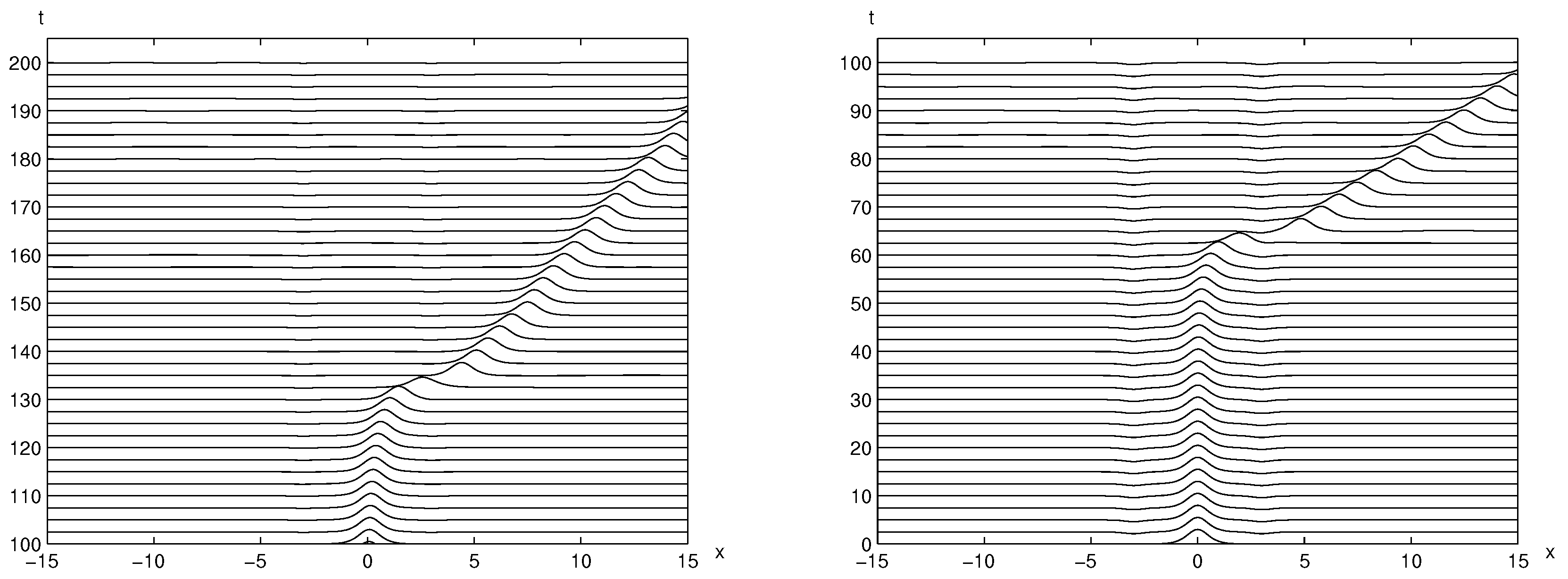
Figure 5.
The time evolution of the trapped solitary wave solution is displayed with and . The unperturbed trapped solitary wave remains stable between two bumps for a very long time (simulated up to ).
Figure 5.
The time evolution of the trapped solitary wave solution is displayed with and . The unperturbed trapped solitary wave remains stable between two bumps for a very long time (simulated up to ).

Figure 6.
The time evolution of the trapped solitary wave solution is shown for and with perturbation (left) and perturbation (right), respectively. The perturbed trapped solitary waves bounce between two bumps for a long time (shown up to ).
Figure 6.
The time evolution of the trapped solitary wave solution is shown for and with perturbation (left) and perturbation (right), respectively. The perturbed trapped solitary waves bounce between two bumps for a long time (shown up to ).

Figure 7.
Stationary trapped solitary wave solutions are displayed using three different bump sizes, , and when the distance between two bumps is 2 (left) and 4 (right), respectively.
Figure 7.
Stationary trapped solitary wave solutions are displayed using three different bump sizes, , and when the distance between two bumps is 2 (left) and 4 (right), respectively.

Figure 8.
The time evolution of the trapped solitary wave solution using and with perturbation (left) and perturbation (right), respectively. They start moving between two bumps and evolve out of two bumps around and , respectively.
Figure 8.
The time evolution of the trapped solitary wave solution using and with perturbation (left) and perturbation (right), respectively. They start moving between two bumps and evolve out of two bumps around and , respectively.

Figure 9.
The time evolution of the trapped solitary wave solution using and with perturbation (left) and perturbation (right), respectively. They start moving between two bumps and evolve out of two bumps around and , respectively.
Figure 9.
The time evolution of the trapped solitary wave solution using and with perturbation (left) and perturbation (right), respectively. They start moving between two bumps and evolve out of two bumps around and , respectively.

Figure 10.
The impact of the bottom configurations is shown on the time when perturbed trapped solitary waves start evolving out of between two bumps (the left panel for the bump size and the right panel for the bump distance).
Figure 10.
The impact of the bottom configurations is shown on the time when perturbed trapped solitary waves start evolving out of between two bumps (the left panel for the bump size and the right panel for the bump distance).

Figure 11.
Stationary trapped solitary wave solutions are shown using three two-hole configurations with three different distances, , and , respectively.
Figure 11.
Stationary trapped solitary wave solutions are shown using three two-hole configurations with three different distances, , and , respectively.

Figure 12.
Stationary trapped solitary wave solutions are displayed using three different hole sizes, , and when the distance between two holes is 2 (left) and 4 (right), respectively.
Figure 12.
Stationary trapped solitary wave solutions are displayed using three different hole sizes, , and when the distance between two holes is 2 (left) and 4 (right), respectively.

Figure 13.
The time evolution of trapped solitary wave solution is displayed with and (left) and (right), respectively. The unperturbed trapped solitary wave remains stable between two holes for a very short time (see the left panel). It remains for a longer time when the distance increases (stable up to in the right panel).

Figure 14.
The time evolution of trapped solitary wave solution with and (left) and (right), respectively. The unperturbed trapped solitary wave remains stable between two holes up to (see the left panel). It remains for a shorter time when the depth of holes increases to (stable up to in the right panel).

© 2018 by the author. Licensee MDPI, Basel, Switzerland. This article is an open access article distributed under the terms and conditions of the Creative Commons Attribution (CC BY) license (http://creativecommons.org/licenses/by/4.0/).
Share and Cite
MDPI and ACS Style
Lee, S. Dynamics of Trapped Solitary Waves for the Forced KdV Equation. Symmetry 2018, 10, 129. https://0-doi-org.brum.beds.ac.uk/10.3390/sym10050129
AMA Style
Lee S. Dynamics of Trapped Solitary Waves for the Forced KdV Equation. Symmetry. 2018; 10(5):129. https://0-doi-org.brum.beds.ac.uk/10.3390/sym10050129
Chicago/Turabian StyleLee, Sunmi. 2018. "Dynamics of Trapped Solitary Waves for the Forced KdV Equation" Symmetry 10, no. 5: 129. https://0-doi-org.brum.beds.ac.uk/10.3390/sym10050129
Note that from the first issue of 2016, this journal uses article numbers instead of page numbers. See further details here.