Computing Zagreb Indices and Zagreb Polynomials for Symmetrical Nanotubes

Abstract

Topological indices are numbers related to sub-atomic graphs to allow quantitative structure-movement/property/danger connections. These topological indices correspond to some specific physico-concoction properties such as breaking point, security, strain vitality of chemical compounds. The idea of topological indices were set up in compound graph hypothesis in view of vertex degrees. These indices are valuable in the investigation of mitigating exercises of specific Nanotubes and compound systems. In this paper, we discuss Zagreb types of indices and Zagreb polynomials for a few Nanotubes covered by cycles.

1. Introduction

Mathematical chemistry becomes an interesting branch of science in which we talk about and foresee the concoction structure by utilizing numerical apparatuses and does not really allude to the quantum mechanics. As a branch of numerical science where we apply devices of graph hypothesis, chemical graph theory was introduced and extensively studied to show the compound wonder scientifically. This is more imperative to state that the hydrogen particles are regularly overlooked in any sub-atomic graph. Topological indices are really a numeric measures related to the constitution synthetic material implying for relationship of concoction structure with numerous physio-substance features, compound responsiveness or biological activity. Motivated by the wide applications of topological indices, the topological indices of graphs are studied extensively [1,2,3].

A nano structure is a question of middle size among both molecular and microscopic structures. Such a material is determined through designing at atomic scale, which is something that has a physical measurement littler than one hundred nanometers, running from bunches of particles to many dimensional layers. Carbon Nanotubes (CNTs) with allotropes of carbon whose shapes are usually hollow and round possess some kinds of nanostructure.

For a graph G, the degree of a vertex w is the cardinality of edges incident to w and denoted by $dgr\left(s\right)$. A molecular graph is a basic limited graph in which vertices mean the atoms and edges indicate the compound bonds in fundamental substance structures.

For a graph G, a topological index $Tp\left(G\right)$ is a value which can be obtained by a computing method from G. Moreover, if graphs G and F are isomorphic, then the result $Tp\left(F\right)=Tp\left(G\right)$ holds. Wiener [4] initially figured out an idea for a topological index in the early years, and at that time, he took a shot at breaking point of paraffin. He defined this record to be the way number. Afterwards, such a concept was renamed the Wiener index. As we know, the Wiener record is the first posed index and it is one of the most attractive indices, from not only a hypothetical perspective but applications, and characterized as the total of separations among vertices in G, see for subtle elements [5].

The first Zagreb index, a very old topological index, was initiated in 1972 [6] and later many variations of Zagreb index were proposed, e.g., Shirdel et al. [7] in 2013 described a novel index under the name of “hyper-Zagreb index” and it was defined to be

$$HM\left(G\right)=\sum _{sr\in E\left(G\right)}{\left[dgr\left(s\right)+dgr\left(r\right)\right]}^2$$

(1)

in [8], two new versions of Zagreb indices were put forward, which are the first multiple Zagreb index $P{M}_1\left(G\right)$ and the second multiple Zagreb index $P{M}_2\left(G\right)$. More precisely, they are formulated as follows.

$$P{M}_1\left(G\right)=\prod _{sr\in E\left(G\right)}[dgr\left(s\right)+dgr\left(r\right)]$$

(2)

$$P{M}_2\left(G\right)=\prod _{sr\in E\left(G\right)}[dgr\left(s\right)\times dgr\left(r\right)]$$

(3)

Some properties of the indices $P{M}_1\left(G\right),P{M}_2\left(G\right)$ of specific chemical structures were investigated in [9].

To investigate more interesting properties of $P{M}_1\left(G\right),P{M}_2\left(G\right)$ of a graph G, the first Zagreb Polynomial $M_1(G,x)$ and the second Zagreb Polynomial $M_2(G,x)$ are proposed [10,11] and put forward as

$$M_1(G,x)=\sum _{sr\in E\left(G\right)}{x}^{\left[dgr\right(s)+dgr(r\left)\right]}$$

(4)

$$M_2(G,x)=\sum _{sr\in E\left(G\right)}{x}^{\left[dgr\right(s)\times dgr(r\left)\right]}$$

(5)

2. Applications of Nanostructure and Topological Indices

In the past few decades, graph theory was widely applied as a tool to study physical and chemical properties of materials. More and more people are interested in this field and as a result chemical graph theory was introduces, and later various topological indices were studied and defined. Moreover, as a combination of chemistry, mathematics and nano science, nanotechnology was also studied by means of chemical graph theory. Among these, quantitative structure–activity relationship (QSAR) and quantitative structure-property relationship (QSPR) are analyzed to predict the properties of nanostructure and biological activities. To study QSAR and QSPR, hyper-Zagreb index, first multiple Zagreb index, second multiple Zagreb index and Zagreb polynomials are applied to predict the bioactivity of nanostructures [12,13,14,15].

The Zagreb index is defined to be a topological descriptor which is related to substantial synthetic qualities of the atoms [16]. The particle bond network hyper Zagreb index gives a decent connection to the security of direct dendrimers and also the stretched pharmacies and for processing the strain vitality of cyclo alkanes [17,18,19,20,21]. To relate with some physico-concoction properties, multiple Zagreb index bears much preferred prescient control over the prescient energy of the dendrimers [22,23,24]. The first and second Zagreb indices were revealed to be used to research the $\pi$-electron energy of various microscopic particles [25,26,27].

3. ${\mathit{HAC}}_{\mathit{5}}{\mathit{C}}_{\mathit{7}}[\mathit{p},\mathit{q}]$ Nanotube

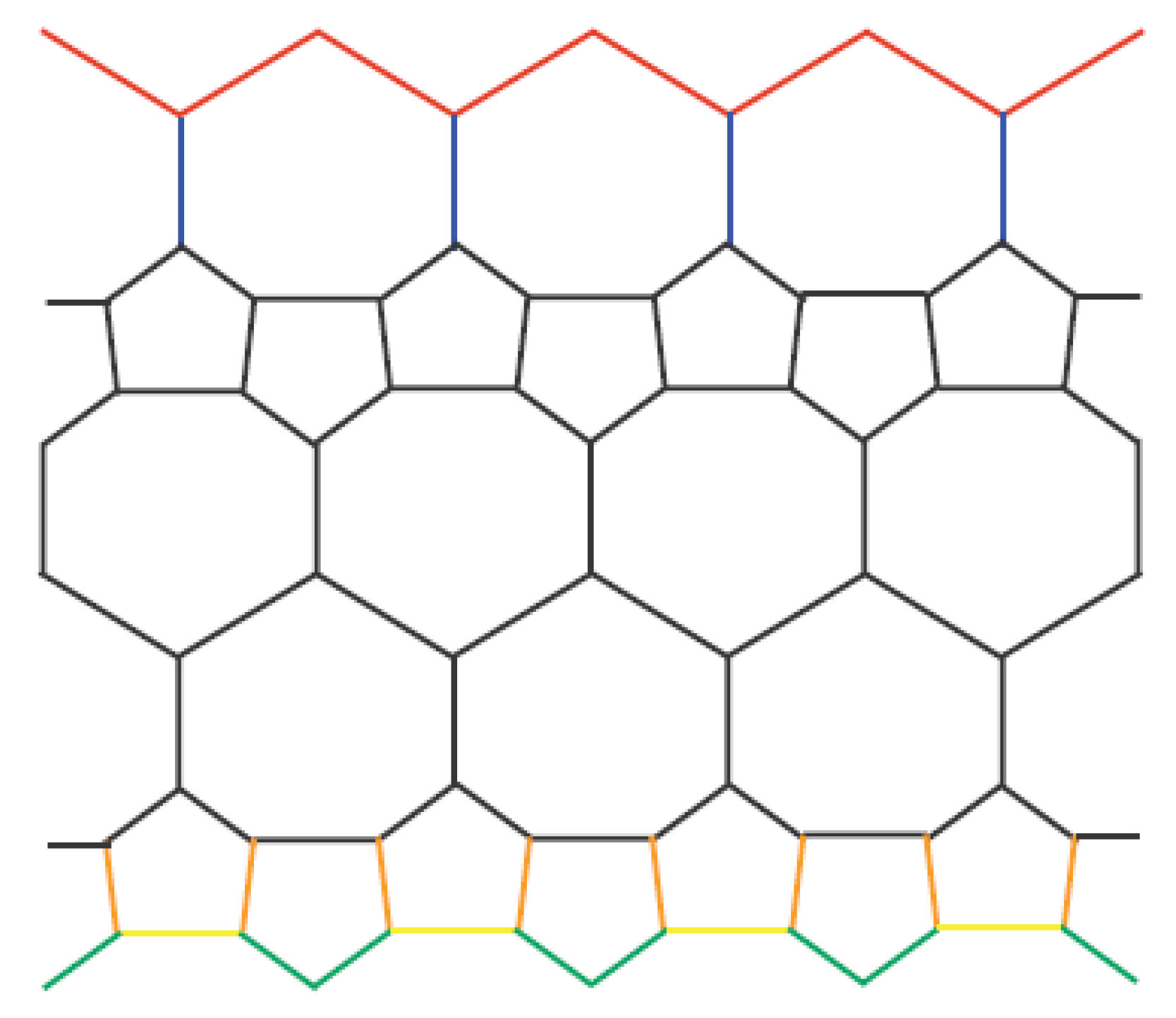
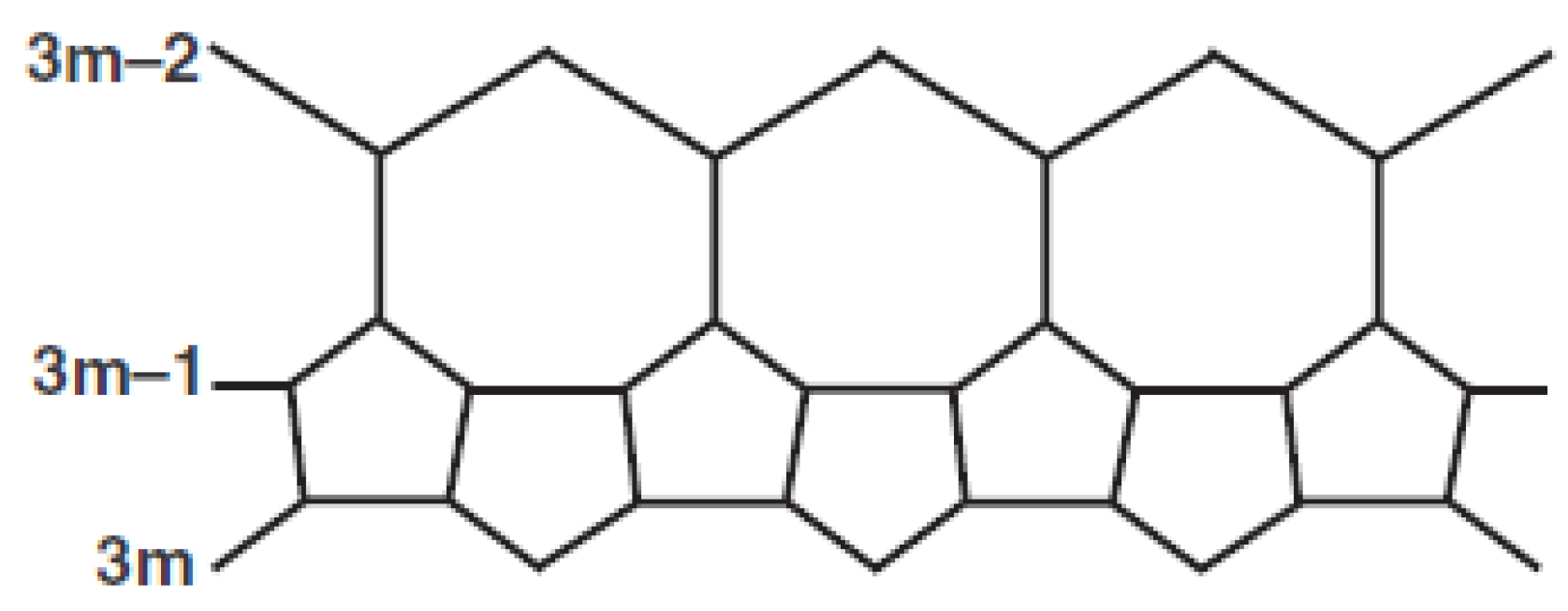
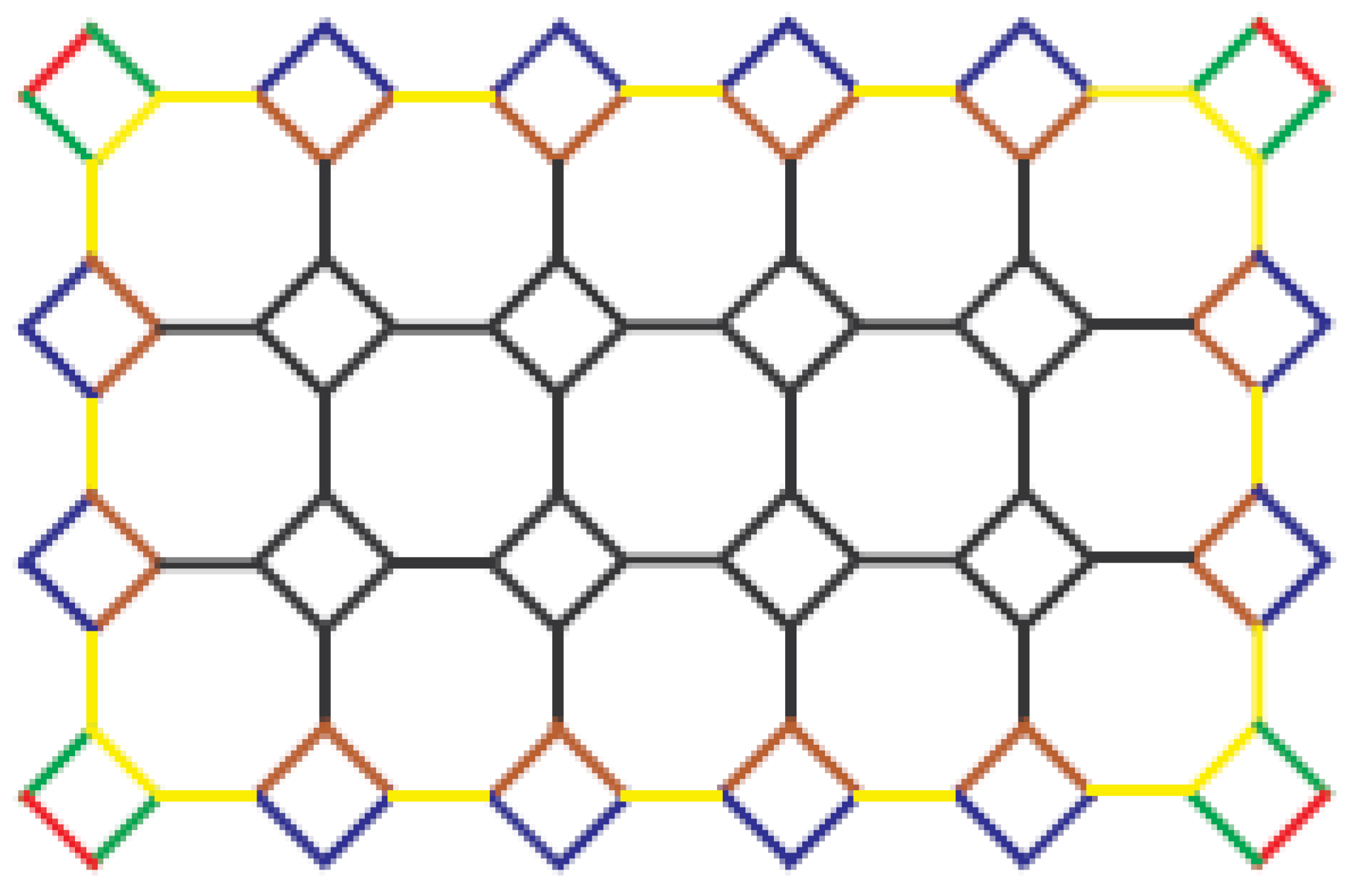
The $HA{C}_5{C}_7[p,q]$ Nanotube can be studied as a $C_5{C}_7$ net and it consists of $C_5$s and $C_7$s with the trivalent decorations. An example is presented in Figure 1, which can be decorated in a cylindrical or toroidal manner. The 2-dimensional lattice of $HA{C}_5{C}_7[p,q]$ were ever been discussed in [28], in which p and q are the cardinalites of heptagons in one row and periods in whole lattice, respectively. As an example, such a Nanotube with three rows is presented in Figure 2.

3.1. Methodology of $HA{C}_5{C}_7[p,q]$ Nanotube Formulas

In the Nanotube $HA{C}_5{C}_7[p,q],(p,q\ge 1)$, we have that $V\left(HA{C}_5{C}_7[p,q]\right)=8pq+p$ and $E\left(HA{C}_5{C}_7[p,q]\right)=12pq-p$. The cardinality of vertices of degree two and three are $2p+2$ and $8pq-p-2$, respectively. According to their sum the the degree over its neighbors of each vertex, the edge set can be partitioned to six disjoint sets as follows.

• $E_1\left(HA{C}_5{C}_7[p,q]\right)=\left\{sr\in E\left(HA{C}_5{C}_7[p,q]\right)\mid dgr\left(s\right)=6,dgr\left(r\right)=7\right\}$
• $E_2\left(HA{C}_5{C}_7[p,q]\right)=\left\{sr\in E\left(HA{C}_5{C}_7[p,q]\right)\mid dgr\left(s\right)=6,dgr\left(r\right)=8\right\}$
• $E_3\left(HA{C}_5{C}_7[p,q]\right)=\left\{sr\in E\left(HA{C}_5{C}_7[p,q]\right)\mid dgr\left(s\right)=7,dgr\left(r\right)=9\right\}$
• $E_4\left(HA{C}_5{C}_7[p,q]\right)=\left\{sr\in E\left(HA{C}_5{C}_7[p,q]\right)\mid dgr\left(s\right)=8,dgr\left(r\right)=8\right\}$
• $E_5\left(HA{C}_5{C}_7[p,q]\right)=\left\{sr\in E\left(HA{C}_5{C}_7[p,q]\right)\mid dgr\left(s\right)=8,dgr\left(r\right)=9\right\}$
• $E_6\left(HA{C}_5{C}_7[p,q]\right)=\left\{sr\in E\left(HA{C}_5{C}_7[p,q]\right)\mid dgr\left(s\right)=9,dgr\left(r\right)=9\right\}$

The cardinality of edges in $E_1\left(HA{C}_5{C}_7[p,q]\right)$, $E_2\left(HA{C}_5{C}_7[p,q]\right)$ and $E_5\left(HA{C}_5{C}_7[p,q]\right)$ are $2p$. The cardinality of edges in $E_3\left(HA{C}_5{C}_7[p,q]\right)$ and $E_4\left(HA{C}_5{C}_7[p,q]\right)$ are p. The cardinality of edges in $E_6\left(HA{C}_5{C}_7[p,q]\right)$ is $12pq-9p$. Such a partition is shown in Figure 1 in which red, green, blue, yellow, brown and black edges are the edges belong to $E_1\left(HA{C}_5{C}_7[p,q]\right)$, $E_2\left(HA{C}_5{C}_7[p,q]\right)$, $E_3\left(HA{C}_5{C}_7[p,q]\right)$, $E_4\left(HA{C}_5{C}_7[p,q]\right)$, $E_5\left(HA{C}_5{C}_7[p,q]\right)$ and $E_6\left(HA{C}_5{C}_7[p,q]\right)$ respectively.

3.2. Main Results for $HA{C}_5{C}_7[p,q]$ Nanotube

In this section, we will obtain hyper-Zagreb index $HM\left(G\right)$, first multiple Zagreb index $P{M}_1\left(G\right)$, second multiple Zagreb index $P{M}_2\left(G\right)$, Zagreb polynomials $M_1(G,x)$, $M_2(G,x)$ for $HA{C}_5{C}_7[p,q],(p,q\ge 1)$ Nanotube.

• Hyper Zagreb index of${\mathit{HAC}}_{\mathit{5}}{\mathit{C}}_{\mathit{7}}[\mathit{p},\mathit{q}]$Nanotube
  Let G be the $HA{C}_5{C}_7[p,q]$ Nanotube. Then by Equations (1), we have

  $$\begin{array}{ccc}\hfill HM\left(G\right)& =& \sum _{sr\in E\left(G\right)}{\left[dgr\left(s\right)+dgr\left(r\right)\right]}^2\hfill \\ \hfill HM\left(G\right)& =& \sum _{sr\in E_1}{\left[dgr\left(s\right)+dgr\left(r\right)\right]}^2+\sum _{sr\in E_2}{\left[dgr\left(s\right)+dgr\left(r\right)\right]}^2+\sum _{sr\in E_3}{\left[dgr\left(s\right)+dgr\left(r\right)\right]}^2\hfill \\ & +& \sum _{sr\in E_4}{\left[dgr\left(s\right)+dgr\left(r\right)\right]}^2+\sum _{sr\in E_5}{\left[dgr\left(s\right)+dgr\left(r\right)\right]}^2+\sum _{sr\in E_6}{\left[dgr\left(s\right)+dgr\left(r\right)\right]}^2\hfill \\ & =& {13}^2|E_1|+{14}^2|E_2|+{16}^2|E_3|+{16}^2|E_4|+{17}^2|E_5|+{18}^2\left|E_6\right|\hfill \\ & =& 169\left(2p\right)+196\left(2p\right)+256p+256p+289\left(2p\right)+324(12pq-9p)=3888pq-1092p\hfill \end{array}$$
• Multiple Zagreb indices of${\mathit{HAC}}_{\mathit{5}}{\mathit{C}}_{\mathit{7}}[\mathit{p},\mathit{q}]$Nanotube
  Let G be the $HA{C}_5{C}_7[p,q]$ Nanotube. Then by Equations (2) and (3), we have

  $$\begin{array}{ccc}\hfill P{M}_1\left(G\right)& =& \prod _{sr\in E\left(G\right)}[dgr\left(s\right)+dgr\left(r\right)]\hfill \\ \hfill P{M}_1\left(G\right)& =& \prod _{sr\in E_1}\left[dgr\left(s\right)+dgr\left(r\right)\right]\times \prod _{sr\in E_2}\left[dgr\left(s\right)+dgr\left(r\right)\right]\times \prod _{sr\in E_3}\left[dgr\left(s\right)+dgr\left(r\right)\right]\hfill \\ & \times & \prod _{sr\in E_4}\left[dgr\left(s\right)+dgr\left(r\right)\right]\times \prod _{sr\in E_5}\left[dgr\left(s\right)+dgr\left(r\right)\right]\times \prod _{sr\in E_6}\left[dgr\left(s\right)+dgr\left(r\right)\right]\hfill \\ & =& {13}^{|E_1|}\times {14}^{|E_2|}\times {16}^{|E_3|}\times {16}^{|E_4|}\times {17}^{|E_5|}\times {18}^{|E_6|}\hfill \\ & =& {13}^{2p}\times {14}^{2p}\times {16}^p\times {16}^p\times {17}^{2p}\times {18}^{(12pq-9p)}\hfill \end{array}$$

  $$\begin{array}{ccc}\hfill P{M}_2\left(G\right)& =& \prod _{sr\in E\left(G\right)}[dgr\left(s\right)\times dgr\left(r\right)]\hfill \\ \hfill P{M}_2\left(G\right)& =& \prod _{sr\in E_1}\left[dgr\left(s\right)\times dgr\left(r\right)\right]\times \prod _{sr\in E_2}\left[dgr\left(s\right)\times dgr\left(r\right)\right]\times \prod _{sr\in E_3}\left[dgr\left(s\right)\times dgr\left(r\right)\right]\hfill \\ & \times & \prod _{sr\in E_4}\left[dgr\left(s\right)\times dgr\left(r\right)\right]\times \prod _{sr\in E_5}\left[dgr\left(s\right)\times dgr\left(r\right)\right]\times \prod _{sr\in E_6}\left[dgr\left(s\right)\times dgr\left(r\right)\right]\hfill \\ & =& {42}^{|E_1|}\times {48}^{|E_2|}\times {63}^{|E_3|}\times {64}^{|E_4|}\times {72}^{|E_5|}\times {81}^{|E_6|}\hfill \\ & =& {42}^{2p}\times {48}^{2p}\times {63}^p\times {64}^p\times {72}^{2p}\times {81}^{(12pq-9p)}\hfill \end{array}$$
• Zagreb Polynomials of${\mathit{HAC}}_{\mathit{5}}{\mathit{C}}_{\mathit{7}}[\mathit{p},\mathit{q}]$Nanotube
  Let G be the $HA{C}_5{C}_7[p,q]$ Nanotube. Then by Equations (4) and (5), we have

  $$\begin{array}{ccc}\hfill M_1(G,x)& =& \sum _{sr\in E\left(G\right)}{x}^{\left[dgr\right(s)+dgr(r\left)\right]}\hfill \\ \hfill M_1(G,x)& =& \sum _{sr\in E_1}{x}^{\left[dgr\right(s)+dgr(r\left)\right]}+\sum _{sr\in E_2}{x}^{\left[dgr\right(s)+dgr(r\left)\right]}+\sum _{sr\in E_3}{x}^{\left[dgr\right(s)+dgr(r\left)\right]}\hfill \\ & +& \sum _{sr\in E_4}{x}^{\left[dgr\right(s)+dgr(r\left)\right]}+\sum _{sr\in E_5}{x}^{\left[dgr\right(s)+dgr(r\left)\right]}+\sum _{sr\in E_6}{x}^{\left[dgr\right(s)+dgr(r\left)\right]}\hfill \\ & =& \sum _{sr\in E_1}{x}^{13}+\sum _{sr\in E_2}{x}^{14}+\sum _{sr\in E_3}{x}^{16}+\sum _{sr\in E_4}{x}^{16}+\sum _{sr\in E_5}{x}^{17}+\sum _{sr\in E_6}{x}^{18}\hfill \\ & =& |E_1|x^{13}+|E_2|x^{14}+|E_3|x^{16}+|E_4|x^{16}+|E_5|x^{17}+\left|E_6\right|x^{18}\hfill \\ & =& 2p{x}^{13}+2p{x}^{14}+p{x}^{16}+p{x}^{16}+2p{x}^{17}+(12pq-9p)x^{18}\hfill \end{array}$$

  $$\begin{array}{ccc}\hfill M_2(G,x)& =& \sum _{sr\in E\left(G\right)}{x}^{\left[dgr\right(s)\times dgr(r\left)\right]}\hfill \\ \hfill M_2(G,x)& =& \sum _{sr\in E_1}{x}^{\left[dgr\right(s)\times dgr(r\left)\right]}+\sum _{sr\in E_2}{x}^{\left[dgr\right(s)\times dgr(r\left)\right]}+\sum _{sr\in E_3}{x}^{\left[dgr\right(s)\times dgr(r\left)\right]}\hfill \\ & +& \sum _{sr\in E_4}{x}^{\left[dgr\right(s)\times dgr(r\left)\right]}+\sum _{sr\in E_5}{x}^{\left[dgr\right(s)\times dgr(r\left)\right]}+\sum _{sr\in E_6}{x}^{\left[dgr\right(s)\times dgr(r\left)\right]}\hfill \\ & =& \sum _{sr\in E_1}{x}^{42}+\sum _{sr\in E_2}{x}^{48}+\sum _{sr\in E_3}{x}^{63}+\sum _{sr\in E_4}{x}^{64}+\sum _{sr\in E_5}{x}^{72}+\sum _{sr\in E_6}{x}^{81}\hfill \\ & =& |E_1|x^{42}+|E_2|x^{48}+|E_3|x^{63}+|E_4|x^{64}+|E_5|x^{72}+\left|E_6\right|x^{81}\hfill \\ & =& 2p{x}^{42}+2p{x}^{48}+p{x}^{63}+p{x}^{64}+2p{x}^{72}+(12pq-9p)x^{81}\hfill \end{array}$$

4. ${\mathit{HAC}}_{\mathit{5}}{\mathit{C}}_{\mathit{6}}{\mathit{C}}_{\mathit{7}}[\mathit{p},\mathit{q}]$ Nanotube

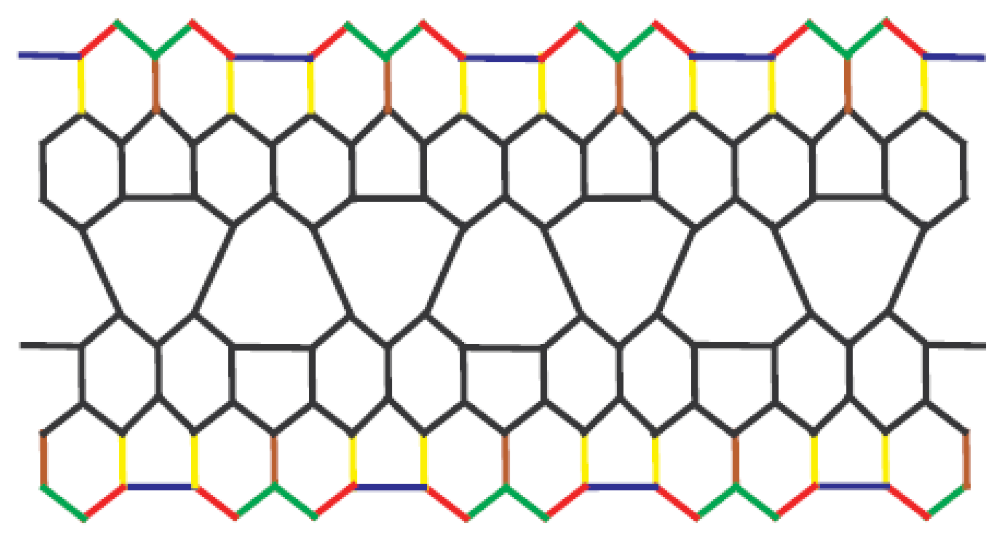
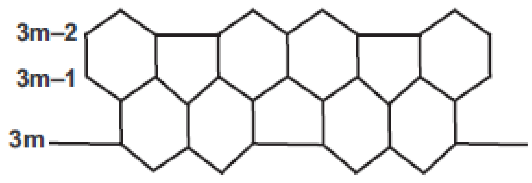
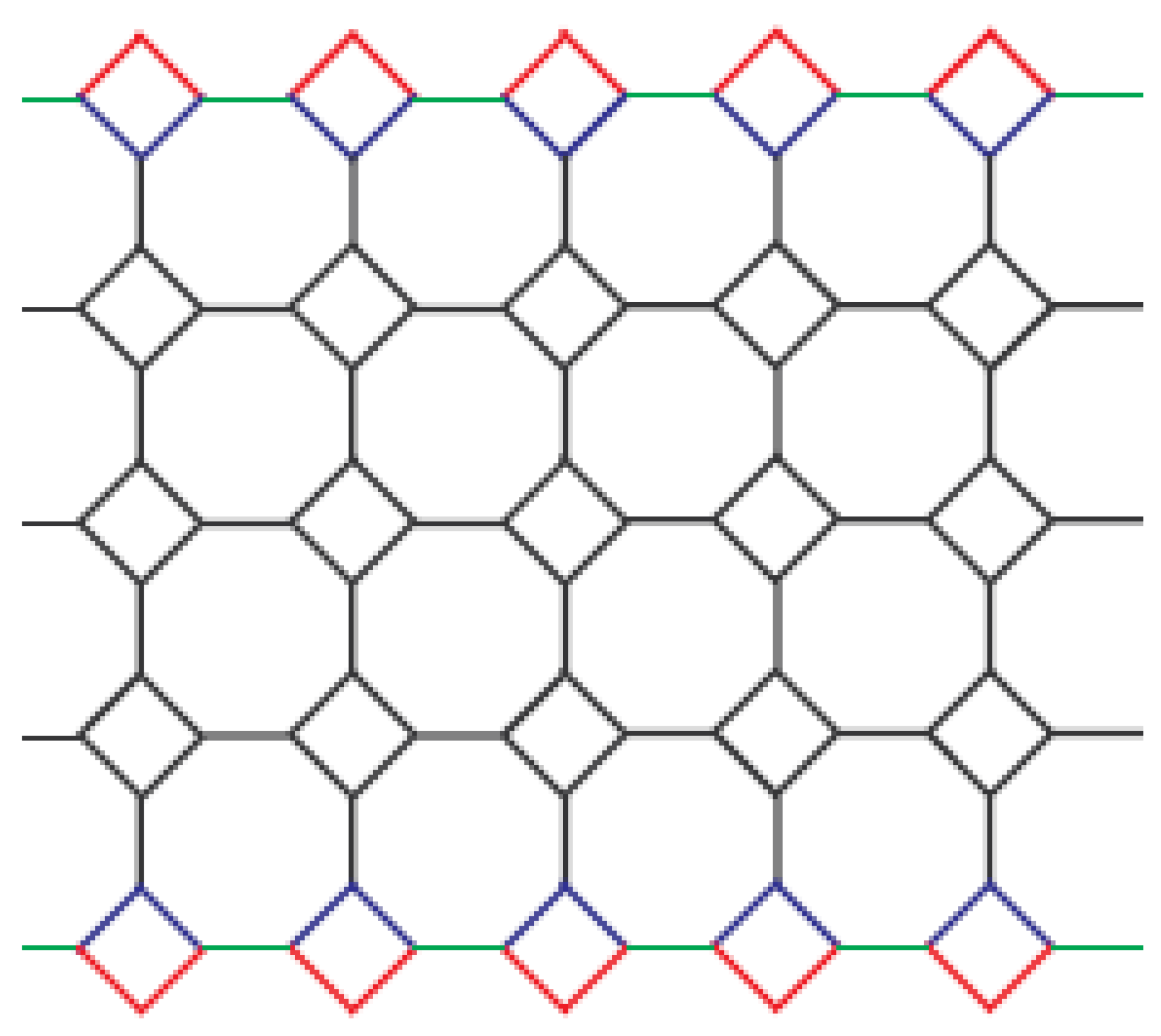
The $HA{C}_5{C}_6{C}_7[p,q]$ Nanotube is a $C_5{C}_6{C}_7$ net and constructed by using $C_{5}s,C_{6}s$ and $C_{7}s$ alternately with the trivalent decorations as demonstrated in Figure 3. These tessellations of $C_{5}s,C_{6}s$ and $C_{7}s$ are usually decorated in a cylindrical or a torodial manner. The 2-dimensional lattice of $HA{C}_5{C}_6{C}_7[p,q]$ is obtained by repeating pentagons for q rows and p columns. The construction of this Nanotube can be found in [29]. As an example, a Nanotube with three rows is shown in Figure 4.

4.1. Methodology of Carbon Graphite $HA{C}_5{C}_6{C}_7[p,q]$ Formulas

For the Nanotube $HA{C}_5{C}_6{C}_7[p,q],(p,q\ge 1)$ (see Figure 2), we have $V\left(HA{C}_5{C}_6{C}_7[p,q]\right)=8pq+p$ and $E\left(HA{C}_5{C}_6{C}_7[p,q]\right)=12pq-p$, and its edge set can be partitioned as follows.

• $E_1\left(HA{C}_5{C}_6{C}_7[p,q]\right)=\left\{sr\in E\left(HA{C}_5{C}_6{C}_7[p,q]\right)\mid dgr\left(s\right)=6,dgr\left(r\right)=7\right\}$
• $E_2\left(HA{C}_5{C}_6{C}_7[p,q]\right)=\left\{sr\in E\left(HA{C}_5{C}_6{C}_7[p,q]\right)\mid dgr\left(s\right)=6,dgr\left(r\right)=8\right\}$
• $E_3\left(HA{C}_5{C}_6{C}_7[p,q]\right)=\left\{sr\in E\left(HA{C}_5{C}_6{C}_7[p,q]\right)\mid dgr\left(s\right)=7,dgr\left(r\right)=8\right\}$
• $E_4\left(HA{C}_5{C}_6{C}_7[p,q]\right)=\left\{sr\in E\left(HA{C}_5{C}_6{C}_7[p,q]\right)\mid dgr\left(s\right)=8,dgr\left(r\right)=8\right\}$
• $E_5\left(HA{C}_5{C}_6{C}_7[p,q]\right)=\left\{sr\in E\left(HA{C}_5{C}_6{C}_7[p,q]\right)\mid dgr\left(s\right)=8,dgr\left(r\right)=9\right\}$
• $E_6\left(HA{C}_5{C}_6{C}_7[p,q]\right)=\left\{sr\in E\left(HA{C}_5{C}_6{C}_7[p,q]\right)\mid dgr\left(s\right)=9,dgr\left(r\right)=9\right\}$

The cardinality of edges in $E_1\left(HA{C}_5{C}_6{C}_7[p,q]\right)$, $E_2\left(HA{C}_5{C}_6{C}_7[p,q]\right)$ and $E_5\left(HA{C}_5{C}_6{C}_7[p,q]\right)$ are $4p$, the cardinality of edges in $E_3\left(HA{C}_5{C}_6{C}_7[p,q]\right)$ and $E_4\left(HA{C}_5{C}_6{C}_7[p,q]\right)$ are $2p$ while the cardinality of edges in $E_6\left(HA{C}_5{C}_6{C}_7[p,q]\right)$ are $24pq-18p$. The representatives of these partitioned edge set are demonstrated in Figure 3, in which the edge set with color green, red, brown, blue, yellow and black are $E_1\left(HA{C}_5{C}_6{C}_7[p,q]\right)$, $E_2\left(HA{C}_5{C}_6{C}_7[p,q]\right)$, $E_3\left(HA{C}_5{C}_6{C}_7[p,q]\right)$, $E_4\left(HA{C}_5{C}_6{C}_7[p,q]\right)$, $E_5\left(HA{C}_5{C}_6{C}_7[p,q]\right)$ and $E_6\left(HA{C}_5{C}_6{C}_7[p,q]\right)$ respectively.

4.2. Main Results for $HA{C}_5{C}_6{C}_7[p,q]$ Nanotube

In this section, we derive hyper-Zagreb index $HM$, first multiple Zagreb index $P{M}_1$, second multiple Zagreb index $P{M}_2$ and Zagreb polynomials for $HA{C}_5{C}_6{C}_7[p,q]$ Nanotube.

• Hyper Zagreb index of${\mathit{HAC}}_{\mathit{5}}{\mathit{C}}_{\mathit{6}}{\mathit{C}}_{\mathit{7}}[\mathit{p},\mathit{q}]$Nanotube
  Let G be the $HA{C}_5{C}_6{C}_7[p,q]$ Nanotube. Then by Equation (1), we have

  $$\begin{array}{ccc}\hfill HM\left(G\right)& =& \sum _{sr\in E\left(G\right)}{\left[dgr\left(s\right)+dgr\left(r\right)\right]}^2\hfill \\ \hfill HM\left(G\right)& =& \sum _{sr\in E_1}{\left[dgr\left(s\right)+dgr\left(r\right)\right]}^2+\sum _{sr\in E_2}{\left[dgr\left(s\right)+dgr\left(r\right)\right]}^2+\sum _{sr\in E_3}{\left[dgr\left(s\right)+dgr\left(r\right)\right]}^2\hfill \\ & +& \sum _{sr\in E_4}{\left[dgr\left(s\right)+dgr\left(r\right)\right]}^2+\sum _{sr\in E_5}{\left[dgr\left(s\right)+dgr\left(r\right)\right]}^2+\sum _{sr\in E_6}{\left[dgr\left(s\right)+dgr\left(r\right)\right]}^2\hfill \\ & =& {13}^2|E_1|+{14}^2|E_2|+{15}^2|E_3|+{16}^2|E_4|+{17}^2|E_5|+{18}^2\left|E_6\right|\hfill \\ & =& 169\left(4p\right)+196\left(4p\right)+225\left(2p\right)+256\left(2p\right)+289\left(4p\right)+324(24pq-18p)\hfill \\ & =& 7776pq-2254p\hfill \end{array}$$
• Multiple Zagreb indices of${\mathit{HAC}}_{\mathit{5}}{\mathit{C}}_{\mathit{6}}{\mathit{C}}_{\mathit{7}}[\mathit{p},\mathit{q}]$Nanotube
  Let G be the $HA{C}_5{C}_6{C}_7[p,q]$ Nanotube. Then by Equations (2) and (3), we have

  $$\begin{array}{ccc}\hfill P{M}_1\left(G\right)& =& \prod _{sr\in E\left(G\right)}[dgr\left(s\right)+dgr\left(r\right)]\hfill \\ \hfill P{M}_1\left(G\right)& =& \prod _{sr\in E_1}\left[dgr\left(s\right)+dgr\left(r\right)\right]\times \prod _{sr\in E_2}\left[dgr\left(s\right)+dgr\left(r\right)\right]\times \prod _{sr\in E_3}\left[dgr\left(s\right)+dgr\left(r\right)\right]\hfill \\ & \times & \prod _{sr\in E_4}\left[dgr\left(s\right)+dgr\left(r\right)\right]\times \prod _{sr\in E_5}\left[dgr\left(s\right)+dgr\left(r\right)\right]\times \prod _{sr\in E_6}\left[dgr\left(s\right)+dgr\left(r\right)\right]\hfill \\ & =& {13}^{|E_1|}\times {14}^{|E_2|}\times {15}^{|E_3|}\times {16}^{|E_4|}\times {17}^{|E_5|}\times {18}^{|E_6|}\hfill \\ & =& {13}^{4p}\times {14}^{4p}\times {15}^{2p}\times {16}^{2p}\times {17}^{4p}\times {18}^{(24pq-18p)}\hfill \end{array}$$

  $$\begin{array}{ccc}\hfill P{M}_2\left(G\right)& =& \prod _{sr\in E\left(G\right)}[dgr\left(s\right)\times dgr\left(r\right)]\hfill \\ \hfill P{M}_2\left(G\right)& =& \prod _{sr\in E_1}\left[dgr\left(s\right)\times dgr\left(r\right)\right]\times \prod _{sr\in E_2}\left[dgr\left(s\right)\times dgr\left(r\right)\right]\times \prod _{sr\in E_3}\left[dgr\left(s\right)\times dgr\left(r\right)\right]\hfill \\ & \times & \prod _{sr\in E_4}\left[dgr\left(s\right)\times dgr\left(r\right)\right]\times \prod _{sr\in E_5}\left[dgr\left(s\right)\times dgr\left(r\right)\right]+\prod _{sr\in E_6}\left[dgr\left(s\right)\times dgr\left(r\right)\right]\hfill \\ & =& {42}^{|E_1|}\times {48}^{|E_2|}\times {56}^{|E_3|}\times {64}^{|E_4|}\times {72}^{|E_5|}\times {81}^{|E_6|}\hfill \\ & =& {42}^{4p}\times {48}^{4p}\times {56}^{2p}\times {64}^{2p}\times {72}^{4p}\times {81}^{(24pq-18p)}\hfill \end{array}$$
• Zagreb polynomials of${\mathit{HAC}}_{\mathit{5}}{\mathit{C}}_{\mathit{6}}{\mathit{C}}_{\mathit{7}}[\mathit{p},\mathit{q}]$Nanotube
  Let G be the graph of $HA{C}_5{C}_6{C}_7[p,q]$ Nanotube. Then by Equations (4) and (5), we have

  $$\begin{array}{ccc}\hfill M_1(G,x)& =& \sum _{sr\in E\left(G\right)}{x}^{\left[dgr\right(s)+dgr(r\left)\right]}\hfill \\ \hfill M_1(G,x)& =& \sum _{sr\in E_1}{x}^{\left[dgr\right(s)+dgr(r\left)\right]}+\sum _{sr\in E_2}{x}^{\left[dgr\right(s)+dgr(r\left)\right]}+\sum _{sr\in E_3}{x}^{\left[dgr\right(s)+dgr(r\left)\right]}\hfill \\ & +& \sum _{sr\in E_4}{x}^{\left[dgr\right(s)+dgr(r\left)\right]}+\sum _{sr\in E_5}{x}^{\left[dgr\right(s)+dgr(r\left)\right]}+\sum _{sr\in E_6}{x}^{\left[dgr\right(s)+dgr(r\left)\right]}\hfill \\ & =& \sum _{sr\in E_1}{x}^{13}+\sum _{sr\in E_2}{x}^{14}+\sum _{sr\in E_3}{x}^{16}+\sum _{sr\in E_4}{x}^{16}+\sum _{sr\in E_5}{x}^{17}+\sum _{sr\in E_6}{x}^{18}\hfill \\ & =& |E_1|x^{13}+|E_2|x^{14}+|E_3|x^{15}+|E_4|x^{16}+|E_5|x^{17}+\left|E_6\right|x^{18}\hfill \\ & =& 4p{x}^{13}+4p{x}^{14}+2p{x}^{15}+2p{x}^{16}+4p{x}^{17}+(24pq-18p)x^{18}\hfill \end{array}$$

  $$\begin{array}{ccc}\hfill M_2(G,x)& =& \sum _{sr\in E\left(G\right)}{x}^{\left[dgr\right(s)\times dgr(r\left)\right]}\hfill \\ \hfill M_2(G,x)& =& \sum _{sr\in E_1}{x}^{\left[dgr\right(s)\times dgr(r\left)\right]}+\sum _{sr\in E_2}{x}^{\left[dgr\right(s)\times dgr(r\left)\right]}+\sum _{sr\in E_3}{x}^{\left[dgr\right(s)\times dgr(r\left)\right]}\hfill \\ & +& \sum _{sr\in E_4}{x}^{\left[dgr\right(s)\times dgr(r\left)\right]}+\sum _{sr\in E_5}{x}^{\left[dgr\right(s)\times dgr(r\left)\right]}+\sum _{sr\in E_6}{x}^{\left[dgr\right(s)\times dgr(r\left)\right]}\hfill \\ & =& \sum _{sr\in E_1}{x}^{42}+\sum _{sr\in E_2}{x}^{48}+\sum _{sr\in E_3}{x}^{56}+\sum _{sr\in E_4}{x}^{64}+\sum _{sr\in E_5}{x}^{72}+\sum _{sr\in E_6}{x}^{81}\hfill \\ & =& |E_1|x^{42}+|E_2|x^{48}+|E_3|x^{56}+|E_4|x^{64}+|E_5|x^{72}+\left|E_6\right|x^{81}\hfill \\ & =& 4p{x}^{42}+4p{x}^{48}+2p{x}^{56}+2p{x}^{64}+4p{x}^{72}+(24pq-18p)x^{81}\hfill \end{array}$$

5. ${\mathit{TUC}}_{\mathit{4}}{\mathit{C}}_{\mathit{8}}[\mathit{p},\mathit{q}]$ Nanotube and Nanotorus

We will use the notations and notions of Diudea and Graovac, and the 2D lattice of $TU{C}_4{C}_8[p,q]$ Nanotorus is denoted by $KTUC[p,q]$ (see Figure 5) and the $TU{C}_4{C}_8[p,q]$ Nanotube is denoted by $GTUC[p,q]$ (see Figure 6). A $TU{C}_4{C}_8[p,q]$ Nanotube is constructed in such a way that the total cardinality of octagons in each row equalsp p and the total cardinality of octagons in each column equals q. An example is presented in Figure 6. In $TU{C}_4{C}_8[p,q]$ Nanotube, the total cardinality of octagons and squares are the same as those in each row, and in $TU{C}_4{C}_8[p,q]$ Nanotorus the total cardinality of octagons and squares are the same as those in each row and column. In 2D lattice of $TU{C}_4{C}_8[p,q]$ Nanotorus, the total cardinality of squares in rows and columns are $(p+1)$ and $(q+1)$, respectively (cf. [30,31]).

The cardinalities of the vertex and edge set of $KTUC[p,q]$ and $GTUC[p,q]$ are presented in the following

Table 1. Order and size of Nanotorus $KTUC[p,q]$ and Nanotube $GTUC[p,q]$.

${\mathit{TUC}}_4{\mathit{C}}_8[\mathit{p},\mathit{q}]$	$\mathit{KTUC}[\mathit{p},\mathit{q}]$	$\mathit{GTUC}[\mathit{p},\mathit{q}]$
$\left|V\right|$	$(4p^2+4p)(q+1)$	$4pq+4p$
$\left|E\right|$	$6pq+5p+5q+4$	$6pq+5p$

.

5.1. Methodology of $KTUC[p,q],(p,q\ge 1)$ Nanotorus Formulas

For the Nanotorus $KTUC[p,q],(p,q\ge 1)$, we have that the number of vertices in $KTUC[p,q]$ is $4p(p+1)(q+1)$ and the number of edges is $6pq+5(p+q)+4$. The edge set can be partitioned into the following six disjoint sets:

• $E_1\left(KTUC[p,q]\right)=\left\{sr\in E\left(KTUC[p,q]\right)\mid dgr\left(s\right)=5,dgr\left(r\right)=5\right\}$
• $E_2\left(KTUC[p,q]\right)=\left\{sr\in E\left(KTUC[p,q]\right)\mid dgr\left(s\right)=5,dgr\left(r\right)=8\right\}$
• $E_3\left(KTUC[p,q]\right)=\left\{sr\in E\left(KTUC[p,q]\right)\mid dgr\left(s\right)=6,dgr\left(r\right)=8\right\}$
• $E_4\left(KTUC[p,q]\right)=\left\{sr\in E\left(KTUC[p,q]\right)\mid dgr\left(s\right)=8,dgr\left(r\right)=8\right\}$
• $E_5\left(KTUC[p,q]\right)=\left\{sr\in E\left(KTUC[p,q]\right)\mid dgr\left(s\right)=8,dgr\left(r\right)=9\right\}$
• $E_6\left(KTUC[p,q]\right)=\left\{sr\in E\left(KTUC[p,q]\right)\mid dgr\left(s\right)=9,dgr\left(r\right)=9\right\}$

We can obtain that $|E_1\left(KTUC[p,q]\right)|=4$, $|E_2\left(KTUC[p,q]\right)|=8$, $|E_3\left(KTUC[p,q]\right)|=4(p+q-2)$, $|E_4\left(KTUC[p,q]\right)|=2(p+q+2)$, $|E_5\left(KTUC[p,q]\right)|=4(p+q-2)$ and $|E_6\left(KTUC[p,q]\right)|=6pq-5p-5q+4$, and the representatives of these partitioned edge set are demonstrated in Figure 5, in which the edge set with color red, green, blue, yellow, brown and black are $E_1\left(KTUC[p,q]\right)$, $E_2\left(KTUC[p,q]\right)$, $E_3\left(KTUC[p,q]\right)$, $E_4\left(KTUC[p,q]\right)$, $E_5\left(KTUC[p,q]\right)$ and $E_6\left(KTUC[p,q]\right)$ respectively.

5.2. Main Results for $KTUC[p,q],(p,q\ge 1)$ Nanotorus

• Hyper Zagreb index of$\mathit{KTUC}[\mathit{p},\mathit{q}],(\mathit{p},\mathit{q}\ge \mathit{1})$Nanotorus
  Let $G=KTUC[p,q]$. Now using Equation (1), we have

  $$\begin{array}{ccc}\hfill HM\left(G\right)& =& \sum _{sr\in E\left(G\right)}{\left[dgr\left(s\right)+dgr\left(r\right)\right]}^2\hfill \\ \hfill HM\left(K\right)& =& \sum _{sr\in E_1}{\left[dgr\left(s\right)+dgr\left(r\right)\right]}^2+\sum _{sr\in E_2}{\left[dgr\left(s\right)+dgr\left(r\right)\right]}^2+\sum _{sr\in E_3}{\left[dgr\left(s\right)+dgr\left(r\right)\right]}^2\hfill \\ & +& \sum _{sr\in E_4}{\left[dgr\left(s\right)+dgr\left(r\right)\right]}^2+\sum _{sr\in E_5}{\left[dgr\left(s\right)+dgr\left(r\right)\right]}^2+\sum _{sr\in E_6}{\left[dgr\left(s\right)+dgr\left(r\right)\right]}^2\hfill \\ & =& {10}^2|E_1|+{13}^2|E_2|+{14}^2|E_3|+{16}^2|E_4|+{17}^2|E_5|+{18}^2\left|E_6\right|\hfill \\ & =& 100\left(4\right)+169\left(8\right)+196(4p+4q-8)+256(2p+2q+4)\hfill \\ & +& 289(4p+4q-8)+324(6pq-5p-5q+4)\hfill \\ & =& 1944pq+832(p+q)+192\hfill \end{array}$$
• Multiple Zagreb indices of$\mathit{KTUC}[\mathit{p},\mathit{q}],(\mathit{p},\mathit{q}\ge \mathit{1})$Nanotorus
  Let $G=KTUC[p,q]$. Now using Equations (2) and (3) we have

  $$\begin{array}{ccc}\hfill P{M}_1\left(G\right)& =& \prod _{sr\in E\left(G\right)}[dgr\left(s\right)+dgr\left(r\right)]\hfill \\ \hfill P{M}_1\left(K\right)& =& \prod _{sr\in E_1}\left[dgr\left(s\right)+dgr\left(r\right)\right]\times \prod _{sr\in E_2}\left[dgr\left(s\right)+dgr\left(r\right)\right]\times \prod _{sr\in E_3}\left[dgr\left(s\right)+dgr\left(r\right)\right]\hfill \\ & \times & \prod _{sr\in E_4}\left[dgr\left(s\right)+dgr\left(r\right)\right]\times \prod _{sr\in E_5}\left[dgr\left(s\right)+dgr\left(r\right)\right]\times \prod _{sr\in E_6}\left[dgr\left(s\right)+dgr\left(r\right)\right]\hfill \\ & =& {10}^{|E_1|}\times {13}^{|E_2|}\times {14}^{|E_3|}\times {16}^{|E_4|}\times {17}^{|E_5|}\times {18}^{|E_6|}\hfill \\ & =& {10}^4\times {13}^8\times {14}^{(4p+4q-8)}\times {16}^{(2p+2q+4)}\times {17}^{(4p+4q-8)}\times {18}^{(6pq-5p-5q+4)}\hfill \end{array}$$

  $$\begin{array}{ccc}\hfill P{M}_2\left(G\right)& =& \prod _{sr\in E\left(G\right)}[dgr\left(s\right)\times dgr\left(r\right)]\hfill \\ \hfill P{M}_2\left(K\right)& =& \prod _{sr\in E_1}\left[dgr\left(s\right)\times dgr\left(r\right)\right]\times \prod _{sr\in E_2}\left[dgr\left(s\right)\times dgr\left(r\right)\right]\times \prod _{sr\in E_3}\left[dgr\left(s\right)\times dgr\left(r\right)\right]\hfill \\ & \times & \prod _{sr\in E_4}\left[dgr\left(s\right)\times dgr\left(r\right)\right]\times \prod _{sr\in E_5}\left[dgr\left(s\right)\times dgr\left(r\right)\right]\times \prod _{sr\in E_6}\left[dgr\left(s\right)\times dgr\left(r\right)\right]\hfill \\ & =& {25}^{|E_1|}\times {40}^{|E_2|}\times {48}^{|E_3|}\times {64}^{|E_4|}\times {72}^{|E_5|}\times {81}^{|E_6|}\hfill \\ & =& {25}^4\times {40}^8\times {48}^{(4p+4q-8)}\times {64}^{(2p+2q+4)}\times {72}^{(4p+4q-8)}\times {81}^{(6pq-5p-5q+4)}\hfill \end{array}$$
• Zagreb polynomials of$\mathit{KTUC}[\mathit{p},\mathit{q}],(\mathit{p},\mathit{q}\ge \mathit{1})$Nanotorus
  Let $G=KTUC[p,q]$. Now using Equations (4) and (5) we have

  $$\begin{array}{ccc}\hfill M_1(G,x)& =& \sum _{sr\in E\left(G\right)}{x}^{\left[dgr\right(s)+dgr(r\left)\right]}\hfill \\ \hfill M_1(K,x)& =& \sum _{sr\in E_1}{x}^{\left[dgr\right(s)+dgr(r\left)\right]}+\sum _{sr\in E_2}{x}^{\left[dgr\right(s)+dgr(r\left)\right]}+\sum _{sr\in E_3}{x}^{\left[dgr\right(s)+dgr(r\left)\right]}\hfill \\ & +& \sum _{sr\in E_4}{x}^{\left[dgr\right(s)+dgr(r\left)\right]}+\sum _{sr\in E_5}{x}^{\left[dgr\right(s)+dgr(r\left)\right]}+\sum _{sr\in E_6}{x}^{\left[dgr\right(s)+dgr(r\left)\right]}\hfill \end{array}$$

  $$\begin{array}{ccc}\hfill M_1(K,x)& =& \sum _{sr\in E_1}{x}^{10}+\sum _{sr\in E_2}{x}^{13}+\sum _{sr\in E_3}{x}^{14}+\sum _{sr\in E_4}{x}^{16}+\sum _{sr\in E_5}{x}^{17}+\sum _{sr\in E_6}{x}^{18}\hfill \\ & =& |E_1|x^{10}+|E_2|x^{13}+|E_3|x^{14}+|E_4|x^{16}+|E_5|x^{17}+\left|E_6\right|x^{18}\hfill \\ & =& 4x^{10}+8x^{13}+(4p+4q-8)x^{14}+(2p+2q+4)x^{16}\hfill \\ & +& (4p+4q-8)x^{17}+(6pq-5p-5q+4)x^{18}\hfill \end{array}$$

  $$\begin{array}{ccc}\hfill M_2(G,x)& =& \sum _{sr\in E\left(G\right)}{x}^{\left[dgr\right(s)\times dgr(r\left)\right]}\hfill \\ \hfill M_2(K,x)& =& \sum _{sr\in E_1}{x}^{\left[dgr\right(s)\times dgr(r\left)\right]}+\sum _{sr\in E_2}{x}^{\left[dgr\right(s)\times dgr(r\left)\right]}+\sum _{sr\in E_3}{x}^{\left[dgr\right(s)\times dgr(r\left)\right]}\hfill \\ & +& \sum _{sr\in E_4}{x}^{\left[dgr\right(s)\times dgr(r\left)\right]}+\sum _{sr\in E_5}{x}^{\left[dgr\right(s)\times dgr(r\left)\right]}+\sum _{sr\in E_6}{x}^{\left[dgr\right(s)\times dgr(r\left)\right]}\hfill \\ & =& \sum _{sr\in E_1}{x}^{25}+\sum _{sr\in E_2}{x}^{40}+\sum _{sr\in E_3}{x}^{48}+\sum _{sr\in E_4}{x}^{64}+\sum _{sr\in E_5}{x}^{72}+\sum _{sr\in E_6}{x}^{81}\hfill \\ & =& |E_1|x^{25}+|E_2|x^{40}+|E_3|x^{48}+|E_4|x^{64}+|E_5|x^{72}+\left|E_6\right|x^{81}\hfill \\ & =& 4x^{25}+8x^{40}+(4p+4q-8)x^{48}+(2p+2q+4)x^{64}\hfill \\ & +& (4p+4q-8)x^{72}+(6pq-5p-5q+4)x^{81}\hfill \end{array}$$

5.3. Methodology and Results of $GTUC[p,q],(p,q\ge 1)$ Nanotube Formulas

For the Nanotube $GTUC[p,q],(p,q\ge 1)$, we know that the number of vertices in $GTUC[p,q]$ are $4p(q+1)$ and the number of edges are $6pq+5p$. The edge set can be partitioned into the following four disjoint sets:

• $E_1\left(GTUC[p,q]\right)=\left\{sr\in E\left(GTUC[p,q]\right)\mid dgr\left(s\right)=6,dgr\left(r\right)=8\right\}$
• $E_2\left(GTUC[p,q]\right)=\left\{sr\in E\left(GTUC[p,q]\right)\mid dgr\left(s\right)=8,dgr\left(r\right)=8\right\}$
• $E_3\left(GTUC[p,q]\right)=\left\{sr\in E\left(GTUC[p,q]\right)\mid dgr\left(s\right)=8,dgr\left(r\right)=9\right\}$
• $E_4\left(GTUC[p,q]\right)=\left\{sr\in E\left(GTUC[p,q]\right)\mid dgr\left(s\right)=9,dgr\left(r\right)=9\right\}$

The cardinality of edges in $E_1\left(GTUC[p,q]\right)$ are $4p$, in $E_2\left(GTUC[p,q]\right)$ are $2p$, in $E_3\left(GTUC[p,q]\right)$ are $4p$ and in $E_4\left(GTUC[p,q]\right)$ are $6pq-5p$. The representatives of these edge set partitions are shown in Figure 6 in which red, green, blue and black edges are the edges belong to $E_1\left(GTUC[p,q]\right)$, $E_2\left(GTUC[p,q]\right)$, $E_3\left(GTUC[p,q]\right)$ and $E_4\left(GTUC[p,q]\right)$ respectively. Now using Equations (1)–(5), we have

• Hyper Zagreb index of$\mathit{GTUC}[\mathit{p},\mathit{q}],(\mathit{p},\mathit{q}\ge \mathit{1})$Nanotube
  Let $G=GTUC[p,q]$. Now using Equation (1), we have

  $$\begin{array}{ccc}\hfill HM\left(G\right)& =& \sum _{sr\in E\left(G\right)}{\left[dgr\left(s\right)+dgr\left(r\right)\right]}^2\hfill \\ \hfill HM\left(G\right)& =& \sum _{sr\in E_1}{\left[dgr\left(s\right)+dgr\left(r\right)\right]}^2+\sum _{sr\in E_2}{\left[dgr\left(s\right)+dgr\left(r\right)\right]}^2\hfill \\ & +& \sum _{sr\in E_3}{\left[dgr\left(s\right)+dgr\left(r\right)\right]}^2+\sum _{sr\in E_4}{\left[dgr\left(s\right)+dgr\left(r\right)\right]}^2\hfill \\ & =& {14}^2|E_1|+{16}^2|E_2|+{17}^2|E_3|+{18}^2\left|E_4\right|\hfill \\ & =& 196\left(4p\right)+256\left(2p\right)+289\left(4p\right)+324(6pq-5p)\hfill \\ & =& 1944pq+832p\hfill \end{array}$$
• Multiple Zagreb indices of$\mathit{GTUC}[\mathit{p},\mathit{q}],(\mathit{p},\mathit{q}\ge \mathit{1})$Nanotube
  Let $G=GTUC[p,q]$. Now using Equations (2) and (3) we have

  $$\begin{array}{ccc}\hfill P{M}_1\left(G\right)& =& \prod _{sr\in E\left(G\right)}[dgr\left(s\right)+dgr\left(r\right)]\hfill \\ \hfill P{M}_1\left(G\right)& =& \prod _{sr\in E_1}\left[dgr\left(s\right)+dgr\left(r\right)\right]\times \prod _{sr\in E_2}\left[dgr\left(s\right)+dgr\left(r\right)\right]\hfill \\ & \times & \prod _{sr\in E_3}\left[dgr\left(s\right)+dgr\left(r\right)\right]\times \prod _{sr\in E_4}\left[dgr\left(s\right)+dgr\left(r\right)\right]\hfill \\ & =& {14}^{|E_1|}\times {16}^{|E_2|}\times {17}^{|E_3|}\times {18}^{|E_4|}\hfill \\ & =& {14}^{\left(4p\right)}\times {16}^{\left(2p\right)}\times {17}^{\left(4p\right)}\times {18}^{(6pq-5p)}\hfill \\ \hfill P{M}_2\left(G\right)& =& \prod _{sr\in E\left(G\right)}[dgr\left(s\right)\times dgr\left(r\right)]\hfill \\ \hfill P{M}_2\left(G\right)& =& \prod _{sr\in E_1}\left[dgr\left(s\right)\times dgr\left(r\right)\right]\times \prod _{sr\in E_2}\left[dgr\left(s\right)\times dgr\left(r\right)\right]\hfill \\ & \times & \prod _{sr\in E_3}\left[dgr\left(s\right)\times dgr\left(r\right)\right]\times \prod _{sr\in E_4}\left[dgr\left(s\right)\times dgr\left(r\right)\right]\hfill \\ & =& {48}^{|E_1|}\times {64}^{|E_2|}\times {72}^{|E_3|}\times {81}^{|E_4|}\hfill \\ & =& {48}^{\left(4p\right)}\times {64}^{\left(2p\right)}\times {72}^{\left(4p\right)}\times {81}^{(6pq-5p)}\hfill \end{array}$$
• Zagreb polynomials of$\mathit{GTUC}[\mathit{p},\mathit{q}],(\mathit{p},\mathit{q}\ge \mathit{1})$Nanotube
  Let $G=GTUC[p,q]$. Now using Equations (4) and (5) we have

  $$\begin{array}{ccc}\hfill M_1(G,x)& =& \sum _{sr\in E\left(G\right)}{x}^{\left[dgr\right(s)+dgr(r\left)\right]}\hfill \\ \hfill M_1(G,x)& =& \sum _{sr\in E_1}{x}^{\left[dgr\right(s)+dgr(r\left)\right]}+\sum _{sr\in E_2}{x}^{\left[dgr\right(s)+dgr(r\left)\right]}\hfill \\ & +& \sum _{sr\in E_3}{x}^{\left[dgr\right(s)+dgr(r\left)\right]}+\sum _{sr\in E_4}{x}^{\left[dgr\right(s)+dgr(r\left)\right]}\hfill \\ & =& \sum _{sr\in E_1}{x}^{14}+\sum _{sr\in E_2}{x}^{16}+\sum _{sr\in E_3}{x}^{17}+\sum _{sr\in E_4}{x}^{18}\hfill \end{array}$$

  $$\begin{array}{ccc}\hfill M_1(G,x)& =& |E_1|x^{14}+|E_2|x^{16}+|E_3|x^{17}+\left|E_4\right|x^{18}\hfill \\ & =& \left(4p\right)x^{14}+\left(2p\right)x^{16}+\left(4p\right)x^{17}+(6pq-5p)x^{18}\hfill \\ \hfill M_2(G,x)& =& \sum _{sr\in E\left(G\right)}{x}^{\left[dgr\right(s)\times dgr(r\left)\right]}\hfill \\ \hfill M_2(G,x)& =& \sum _{sr\in E_1}{x}^{\left[dgr\right(s)\times dgr(r\left)\right]}+\sum _{sr\in E_2}{x}^{\left[dgr\right(s)\times dgr(r\left)\right]}\hfill \\ & +& \sum _{sr\in E_3}{x}^{\left[dgr\right(s)\times dgr(r\left)\right]}+\sum _{sr\in E_4}{x}^{\left[dgr\right(s)\times dgr(r\left)\right]}\hfill \\ & =& \sum _{sr\in E_1}{x}^{48}+\sum _{sr\in E_2}{x}^{64}+\sum _{sr\in E_3}{x}^{72}+\sum _{sr\in E_4}{x}^{81}\hfill \\ & =& |E_1|x^{48}+|E_2|x^{64}+|E_3|x^{72}+\left|E_4\right|x^{81}\hfill \\ & =& \left(4p\right)x^{48}+\left(2p\right)x^{64}+\left(4p\right)x^{72}+(6pq-5p)x^{81}\hfill \end{array}$$

6. Comparisons and Discussion

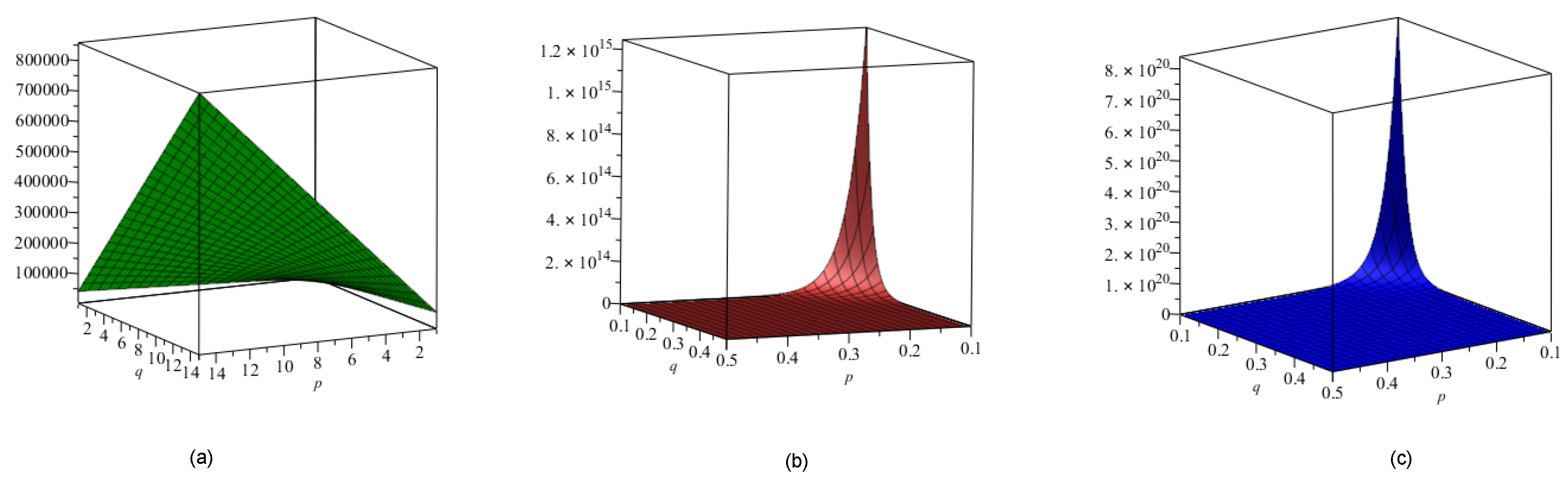
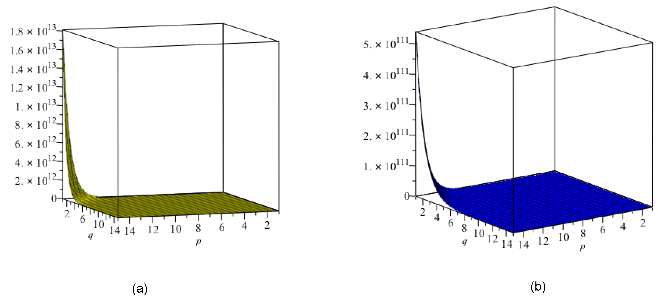
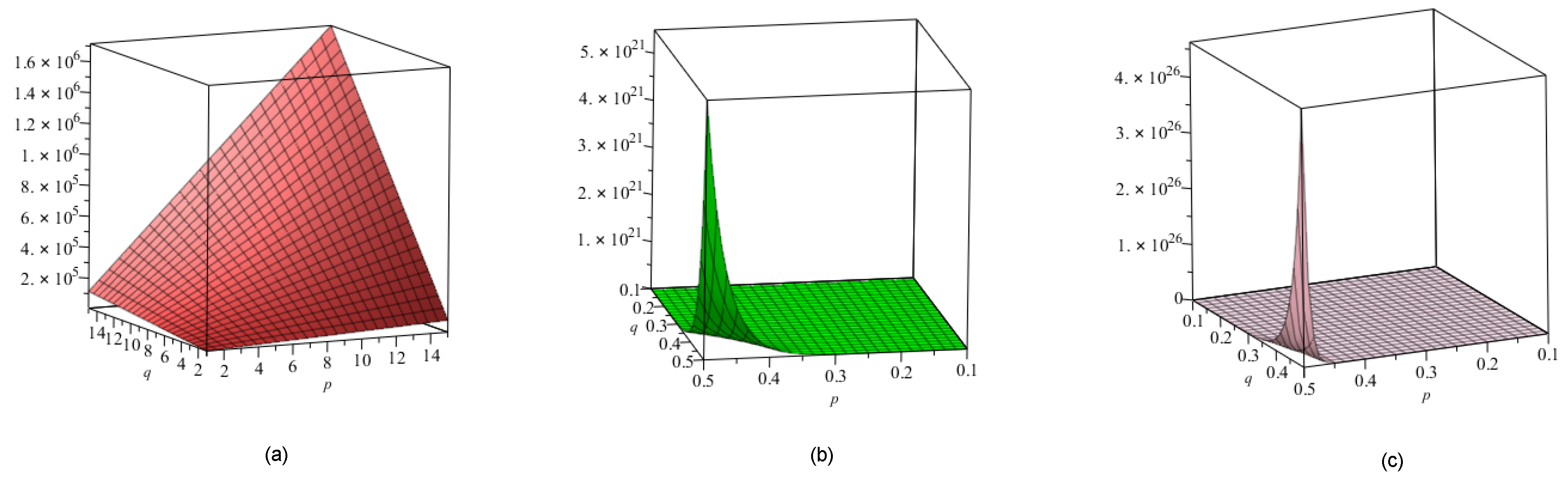
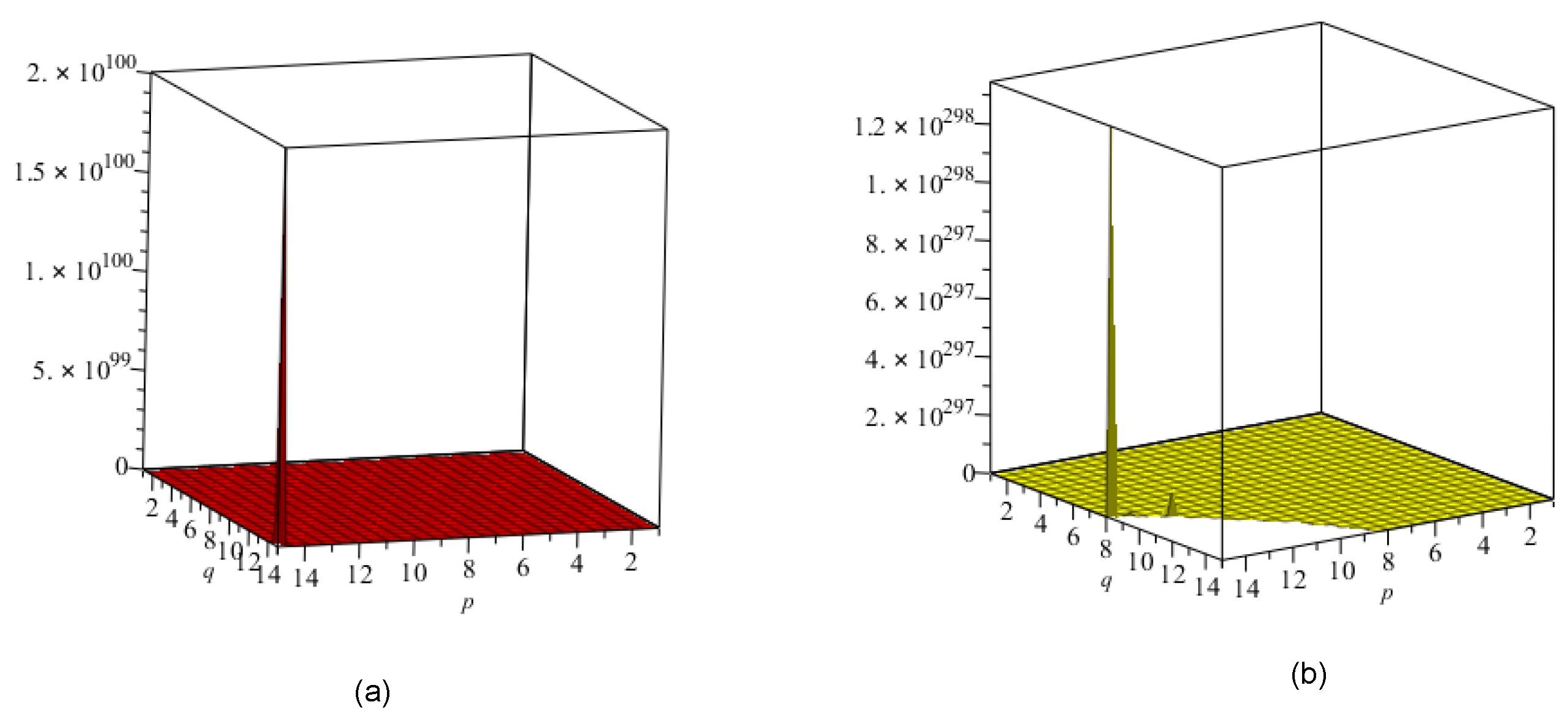
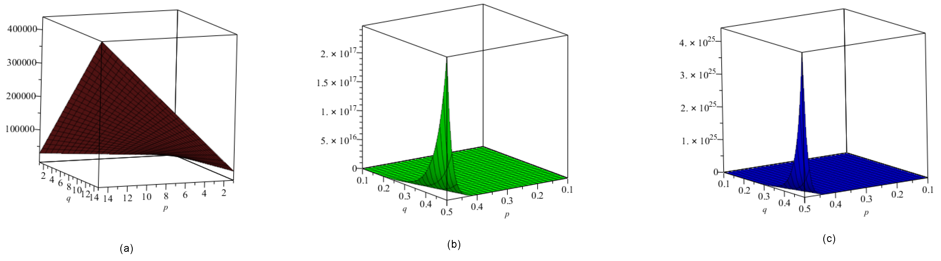
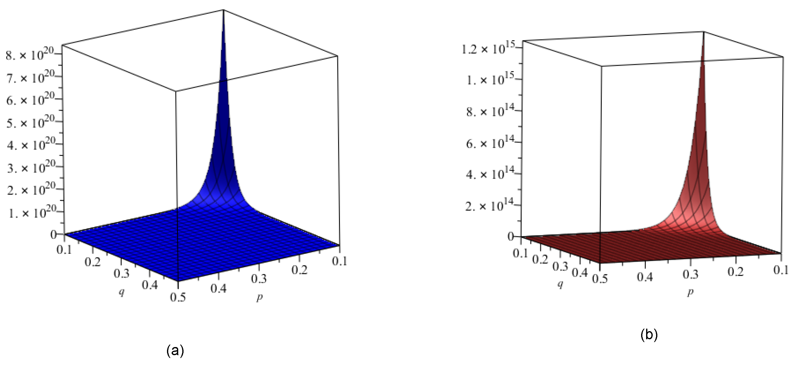
• Firstly, we have obtained some indices of $HA{C}_5{C}_7[p,q]$ Nanotube for any p and q. Now from

  Table 2. Comparison of all indices for $HA{C}_5{C}_7[p,q]$ Nanotube.

  $[\mathit{p},\mathit{q}]$	$\mathit{HM}\left(\mathit{G}\right)$	${\mathit{PM}}_1\left(\mathit{G}\right)$	${\mathit{PM}}_2\left(\mathit{G}\right)$
  $[1,1]$	2796	$2.11\times {10}^{11}$	$3.4\times {10}^{15}$
  $[2,2]$	$13,368$	$3.31\times {10}^{25}$	$4.5\times {10}^{28}$
  $[3,3]$	$31,716$	$4.21\times {10}^{55}$	$6.61\times {10}^{62}$
  $[4,4]$	$57,840$	$6.57\times {10}^{95}$	$8.72\times {10}^{98}$

  , it can be seen that all indices are in increasing order as the values of $p,q$ increase. Finally, we depicted the the graphical representation of $HA{C}_5{C}_7[p,q]$ Nanotube for hyper Zagreb index, first and second multiple Zagreb index in Figure 7 and for first and second Zagreb polynomial in Figure 8.
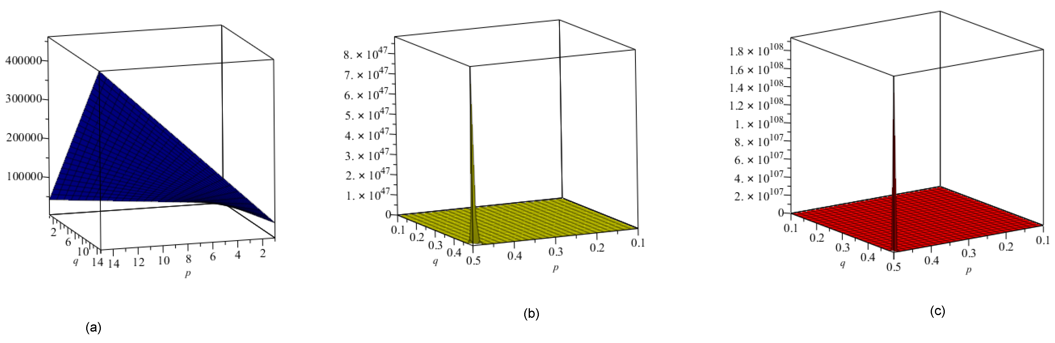
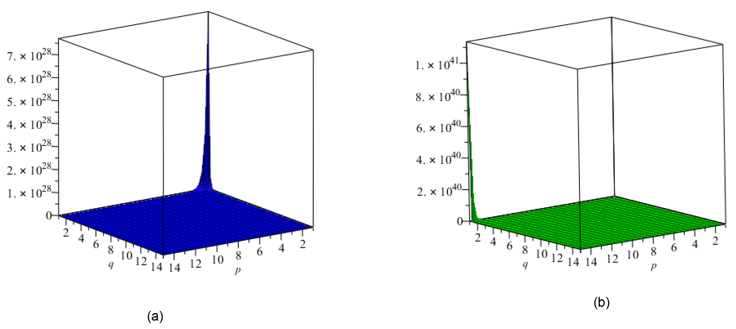
• Secondly, we have worked out many indices of $HA{C}_5{C}_6{C}_7[p,q]$ Nanotube for each p and q. Now from

  Table 3. Comparison of all indices for $HA{C}_5{C}_6{C}_7[p,q]$ Nanotube.

  $[\mathit{p},\mathit{q}]$	$\mathit{HM}\left(\mathit{G}\right)$	${\mathit{PM}}_1\left(\mathit{G}\right)$	${\mathit{PM}}_2\left(\mathit{G}\right)$
  $[1,1]$	5522	$3.4\times {10}^{13}$	$4.5\times {10}^{16}$
  $[2,2]$	$26,596$	$5.3\times {10}^{26}$	$6.5\times {10}^{31}$
  $[3,3]$	$63,222$	$6.31\times {10}^{65}$	$7.62\times {10}^{72}$
  $[4,4]$	$115,400$	$7.57\times {10}^{98}$	$9.82\times {10}^{99}$

  , we can easily see that all indices are in increasing order as the values of $p,q$ increase. Finally, we gave the the graphical representation of $HA{C}_5{C}_6{C}_7[p,q]$ Nanotube for hyper Zagreb index, first and second multiple Zagreb index in Figure 9 and for first and second Zagreb polynomial in Figure 10.
• Now, we have worked out various indices of $KTUC[p,q],(p,q\ge 1)$ Nanotorus with different p and q. Now from

  Table 4. Comparison of all indices for $KTUC[p,q],(p,q\ge 1)$ Nanotorus.

  $[\mathit{p},\mathit{q}]$	$\mathit{HM}\left(\mathit{G}\right)$	${\mathit{PM}}_1\left(\mathit{G}\right)$	${\mathit{PM}}_2\left(\mathit{G}\right)$
  $[1,1]$	2996	$3.2\times {10}^{12}$	$4.5\times {10}^{18}$
  $[2,2]$	$11,296$	$4.6\times {10}^{27}$	$5.7\times {10}^{30}$
  $[3,3]$	$22,680$	$6.8\times {10}^{58}$	$6.21\times {10}^{61}$
  $[4,4]$	$37,952$	$8.7\times {10}^{96}$	$7.8\times {10}^{97}$

  , we have that each index increases with the values of $p,q$ increasing. Finally, we depicted the the graphical representation of $KTUC[p,q],(p,q\ge 1)$ Nanotorus for hyper Zagreb index, first and second multiple Zagreb index in Figure 11 and for first and second Zagreb polynomial in Figure 12.
• At the end of this section, we have computed substantial indices of $GTUC[p,q],(p,q\ge 1)$ Nanotube for different values of $p,q$. Now from

  Table 5. Comparison of all indices for $GTUC[p,q],(p,q\ge 1)$ Nanotube.

  $[\mathit{p},\mathit{q}]$	$\mathit{HM}\left(\mathit{G}\right)$	${\mathit{PM}}_1\left(\mathit{G}\right)$	${\mathit{PM}}_2\left(\mathit{G}\right)$
  $[1,1]$	2776	$1.2\times {10}^{14}$	$2.3\times {10}^{15}$
  $[2,2]$	9440	$3.6\times {10}^{21}$	$4.5\times {10}^{25}$
  $[3,3]$	$19,992$	$5.8\times {10}^{53}$	$5.23\times {10}^{51}$
  $[4,4]$	$34,432$	$7.7\times {10}^{95}$	$6.7\times {10}^{96}$

  , it can be seen that all indices are in increasing order as the values of $p,q$ increase. We also provided the the graphical representation of $GTUC[p,q],(p,q\ge 1)$ Nanotube for hyper Zagreb index, first and second multiple Zagreb index in Figure 13 and for first and second Zagreb polynomial in Figure 14.

7. Conclusions

In this paper, we computed various topological indices of Nanotubes. More precisely, we determined second multiple Zagreb index $P{M}_2\left(G\right)$, hyper-Zagreb index $HM\left(G\right)$, first multiple Zagreb index $P{M}_1\left(G\right)$, and Zagreb polynomials $M_1(G,x)$, $M_2(G,x)$ for certain Nanotubes. We conclude that the the Zagreb indices are in increasing order as the values of $p,q$ increase. In addition, the hyper Zagreb index gives a decent connection to the security of nonstructural objects and the stretched pharmacies, and for processing the strain vitality of Nanotubes. The first and second Zagreb polynomials are helpful to find the features of $\pi$-electron energy of the microscopic particles in the inner part of Nanostructural objects.

References

- Naji, A.M.; Soner, N.D.; Gutman, I. On leap Zagreb indices of graphs. Commun. Comb. Optim. 2017, 2, 99–117. [Google Scholar]
- Shao, Z.; Wu, P.; Gao, Y.; Gutman, I.; Zhang, X. On the maximum ABC index of graphs without pendent vertices. Appl. Math. Comput. 2017, 315, 298–312. [Google Scholar] [CrossRef]
- Shao, Z.; Wu, P.; Zhang, X.; Dimitrov, D.; Liu, J. On the maximum ABC index of graphs with prescribed size and without pendent vertices. IEEE Access 2018, 6, 27604–27616. [Google Scholar] [CrossRef]
- Wiener, H. Structural determination of paraffin boiling points. J. Am. Chem. Soc. 1947, 69, 17–20. [Google Scholar] [CrossRef] [PubMed]
- Dobrynin, A.A.; Entringer, R.; Gutman, I. Wiener index of trees: Theory and applications. Acta Appl. Math. 2001, 66, 211–249. [Google Scholar] [CrossRef]
- Gutman, I.; Trinajstic, N. Graph theory and molecular orbitals. Total ϕ-electron energy of alternant hydrocarbons. Chem. Phys. Lett. 1972, 17, 535–538. [Google Scholar] [CrossRef]
- Shirdel, G.H.; RezaPour, H.; Sayadi, A.M. The hyper-Zagreb Index of Graph Operations. Iran. J. Math. Chem. 2013, 4, 213–220. [Google Scholar]
- Ghorbani, M.; Azimi, N. Note on multiple Zagreb indices. Iran. J. Math. Chem. 2012, 3, 137–143. [Google Scholar]
- Eliasi, M.; Iranmanesh, A.; Gutman, I. Multiplicative version of first Zagreb index. MATCH Commun. Math. Comput. Chem. 2012, 68, 217–230. [Google Scholar]
- Furtula, B.; Gutman, I.; Dehmer, M. On structure-sensitivity of degree-based topological indices. Appl. Math. Comput. 2013, 219, 8973–8978. [Google Scholar] [CrossRef]
- Gutman, I.; Das, K.C. Some Properties of the Second Zagreb Index. MATCH Commun. Math. Comput. Chem. 2004, 50, 103–112. [Google Scholar]
- Farahani, M.R. The hyper zegreb index of TUSC4C8(S) Nanotubes. Int. J. Eng. Technol. Res. 2015, 3, 1–6. [Google Scholar]
- Hayat, S.; Imran, M. Computation of topological indices of certain networks. Appl. Math. Comput. 2014, 240, 213–228. [Google Scholar] [CrossRef]
- Iranmanesh, A.; Alizadeh, Y. Computing wiener index of HAC5C7[p,q] Nanotubes by gap program. Iran. J. Math. Sci. Inform. 2008, 3, 1–12. [Google Scholar]
- Iranmanesh, A.; Zeraatkar, M. Computing ga index of HAC5C7[p,q] and HAC5C6C7[p,q] Nanotubes. Optoelectron. Adv. Mater.-Rapid Commun. 2011, 5, 790–792. [Google Scholar]
- Gao, W.; Siddiqui, M.K.; Naeem, M.; Rehman, N.A. Topological Characterization of Carbon Graphite and Crystal Cubic Carbon Structures. Molecules 2017, 22, 1469. [Google Scholar] [CrossRef] [PubMed]
- Bača, M.; Horváthová, J.; Mokrišová, M.; Suhányiová, A. On topological indices of fullerenes. Appl. Math. Comput. 2015, 251, 154–161. [Google Scholar] [CrossRef]
- Bača, M.; Horváthová, J.; Mokrišová, M.; Semanicová-Fenovcíková, A.; Suhányiová, A. On topological indices of carbon Nanotube network. Can. J. Chem. 2015, 93, 1–4. [Google Scholar] [CrossRef]
- Gao, W.; Farahani, M.R.; Siddiqui, M.K.; Jamil, M.K. On the First and Second Zagreb and First and Second Hyper-Zagreb Indices of Carbon Nanocones CNCk[n]. J. Comput. Theor. Nanosci. 2016, 13, 7475–7482. [Google Scholar] [CrossRef]
- Gao, W.; Farahani, M.R.; Jamil, M.K.; Siddiqui, M.K. The Redefined First, Second and Third Zagreb Indices of Titania Nanotubes TiO2[m,n]. Open Biotechnol. J. 2016, 10, 272–277. [Google Scholar] [CrossRef]
- Gao, W.; Siddiqui, M.K.; Imran, M.; Jamil, M.K.; Farahani, M.R. Forgotten Topological Index of Chemical Structure in Drugs. Saudi Pharm. J. 2016, 24, 258–267. [Google Scholar] [CrossRef] [PubMed]
- Imran, M.; Hayat, S.; Mailk, M.Y.H. On topological indices of certain interconnection networks. Appl. Math. Comput. 2014, 244, 936–951. [Google Scholar] [CrossRef]
- Hayat, S.; Imran, M. Computation of certain topological indices of Nanotubes covered by C5 and C7. J. Comput. Theor. Nanosci. 2015, 12, 1–9. [Google Scholar]
- Imran, M.; Siddiqui, M.K.; Naeem, M.; Iqbal, M.A. On Topological Properties of Symmetric Chemical Structures. Symmetry 2018, 10, 173. [Google Scholar] [CrossRef]
- Siddiqui, M.K.; Gharibi, W. On Zagreb Indices, Zagreb Polynomials of Mesh Derived Networks. J. Comput. Theor. Nanosci. 2016, 13, 8683–8688. [Google Scholar] [CrossRef]
- Siddiqui, M.K.; Imran, M.; Ahmad, A. On Zagreb indices, Zagreb polynomials of some nanostar dendrimers. Appl. Math. Comput. 2016, 280, 132–139. [Google Scholar] [CrossRef]
- Siddiqui, M.K.; Naeem, M.; Rahman, N.A.; Imran, M. Computing topological indicesof certain networks. J. Optoelectron. Adv. Mater. 2016, 18, 884–892. [Google Scholar]
- Mahmiani, A.; Iranmanesh, A. Edge-Szeged Index of HAC5C7[r,p] Nanotube. MATCH Commun. Math. Comput. Chem. 2009, 62, 397–417. [Google Scholar]
- Yazdani, J.; Bahrami, A. Padmakar-Ivan, Omega and Sadhana Polynomial of HAC5C6C7 Nanotubes. Dig. J. Nanomater. Biostruct. 2009, 4, 507–517. [Google Scholar]
- Ashrafi, A.R.; Dosli, T.; Saheli, M. The eccentric connectivity index of TUC4C8(R) Nanotubes. MATCH Commun. Math. Comput. Chem. 2011, 65, 221–230. [Google Scholar]
- Ghorbani, M. Computing ABC4 index of nanostar dendrimers. Optoelectron. Adv. Mater.-Rapid Commun. 2010, 4, 1419–1422. [Google Scholar]
Figure 1.
Nanotube with and .
Figure 2.
The mth period of Nanotube.
Figure 3.
Figure 4.
Figure 5.
2D-lattice of Nanotorus with and .
Figure 6.
Nanotube Nanotube with and .
Figure 7.
(a) Hyper Zagreb index; (b) First multiple Zagreb index; (c) Second multiple Zagreb index.
Figure 8.
(a) First Zagreb polynomial; (b) Second multiple Zagreb polynomial.
Figure 9.
Figure 10.
Figure 11.
Figure 12.
Figure 13.
Figure 14.