Article

Probabilistic Linguistic Preference Relation-Based Decision Framework for Multi-Attribute Group Decision Making

1
School of Computing, SASTRA University, Thanjavur-613401, Tamil Nadu, India
2
Department of Mathematics, National Institute of Technology, Durgapur-713209, West Bengal, India
3
Department of General Studies, Higher College of Technology, Fujairah-4114, UAE
*
Author to whom correspondence should be addressed.
Submission received: 26 November 2018 / Revised: 12 December 2018 / Accepted: 17 December 2018 / Published: 20 December 2018

Abstract

:
With trending competition in decision-making process, linguistic decision-making is gaining attractive attention. Previous studies on linguistic decision-making have neglected the occurring probability (relative importance) of each linguistic term which causes unreasonable ranking of objects. Further, decision-makers’ (DMs) often face difficulties in providing apt preference information for evaluation. Motivated by these challenges, in this paper, we set our proposal on probabilistic linguistic preference relation (PLPR)-based decision framework. The framework consists of two phases viz., (a) missing value entry phase and (b) ranking phase. In phase (a), the missing values of PLPR are filled using a newly proposed automatic procedure and consistency of PLPR is ensured using a consistency check and repair mechanism. Following this, in phase (b), objects are ranked using newly proposed analytic hierarchy process (AHP) method under PLPR context. The practicality of the proposal is validated by using two numerical examples viz., green supplier selection problem for healthcare and the automobile industry. Finally, the strength and weakness of the proposal are discussed by comparing with similar methods.

1. Introduction

Decision-making is an inevitable aspect of human life which involves uncertainty and vagueness. The process of selecting a suitable object for the task brings cognitive thought processes into the picture, which is dynamic and competing in nature [1]. DMs often face difficulties in expressing their opinions in a sensible manner and to alleviate the issue to a certain extent; they adopt linguistic preference information [2]. Previous studies on linguistic decision process [2,3,4] have claimed that (a) linguistic preferences are simple and straightforward information which can be directly obtained from the DM, (b) also, these linguistic preferences mitigate the cost of inaccuracies to some extent. Motivated by these claims; scholars presented different decision-making framework under the linguistic context, of which, some are reviewed here. Zadeh [5] framed the genesis of a linguistic variable and applied the same for approximate reasoning. Later, Herrera et al. [2] fabricated the initial idea of the linguistic decision process and proposed a sequential decision framework in a linguistic environment. Following this, Herrera et al. [3,6] presented the consensus model for group decision-making under the linguistic context. Inspired by the power of linguistic theory, Xu [7] extended the geometric mean and ordered weighted geometric aggregation operator for a linguistic domain. Further, He et al. [8] put forward a new entropy measure for linguistic-based group decision-making.
Though linguistic decision-making is an attractive concept, DMs still face difficulties in rationally rating the objects. The main reason for this difficulty is the cognitive behavior of the human mind, which encourages pair-wise comparative analysis rather than a standalone rating [9]. Motivated by the power of pair-wise comparison and linguistic term set (LTS), Herrera et al. [10,11] proposed the linguistic preference relation (LPR) concept for group decision-making and investigated some choice functions for the same. Following this, Xu [12] put forward some deviation measures for decision-making process under LPR context. Recently, Molinera et al. [13] developed new fuzzy ontologies for linguistic preference information and applied the same for decision-making. Wang and Xu [14] put forward an interactive algorithm for filling the missing LPR values using consistency measures and repaired the consistency of the same using the repairing mechanism.
Inspired by the power of linguistic information and its substantial use in decision-making, Rodriguez [15] proposed the hesitant fuzzy linguistic term set (HFLTS) which is an extension to LTS under hesitant fuzzy environment [16]. The HFLTS allowed DMs to give different choices of preference for the same instance, which managed uncertainty to some extent. Motivated by the power of HFLTS, Zhu and Xu [17] put forward the hesitant fuzzy linguistic preference relation (HFLPR), which is an extension to preference relation under HFLTS context. They also investigated some consistency measures for the same. Following this, Wang and Xu [18] presented the concept of extended hesitant fuzzy preference relation and studied some consistency measures for the same. Wu [19] presented a consensus model based on possibility distribution for HFLPR and validated the applicability of same for decision-making process. Recently, Song and Hu [20] proposed a decision framework for handling incomplete HFLPR and applied the same for real-time group decision-making problem. Tuysuz and Simsek [21] extended the popular AHP method under HFLTS context and applied the same for assessing the performance of cargo factory.
Though the HFLPR is able to manage DMs’ hesitation in preference information, the occurring probability (distribution assessment) of each linguistic term in the decision-making process is neglected. In many practical applications, all linguistic choices by the DM do not bear the same importance and hence, ignoring the occurring probability of each linguistic term is unreasonable and illogical. To circumvent this challenge, Zhang et al. [22] introduced the concept of linguistic distribution assessment (LDA) and associated symbolic proportion for each linguistic term. Later, Pang et al. [23] generalized the idea of LDA by allowing partial ignorance ( i p i 1 ) in preference elicitation and termed it as probabilistic linguistic term set (PLTS) which is an extension to HFLTS with probability concept. Recently, Zhang et al. [24] put forward the concept of incomplete LDA which is similar to PLTS and used in for decision-making. Inspired by the superiority of PLTS in associating occurring probability to each linguistic term; Bai et al. [25] presented a new comparison method use area concept for PLTS. Later, Liao et al. [26] extended the programming model to PLTS for multi-attribute decision-making (MADM). Liu and Teng [27] extended the Muirhead mean aggregation operator to PLTS for group decision-making. Zhang et al. [28,29] put forward the probabilistic linguistic preference relation (PLPR) concept which is an extension to preference relation under PLTS context and some additive consistency and consensus reaching measures were also investigated. Recently, Xie et al. [30] proposed probabilistic uncertain preference relation and applied the same for virtual reality application. Recently, attracted by the power of PLPR, Wu and Liao [31] proposed gain-lost dominance score method under PLTS for consensus reaching. Xie et al. [32] extended AHP (analytic hierarchy process) method and applied the same for assessing the performance of a new area. Since the concept of PLPR just began, we gained motivation to throw some light towards this concept and set our research focus in this direction.
Based on the review conducted above, some genuine challenges/lacunas are identified which are presented in a nutshell below:
(1)
Investigation of decision process using the preference relation proves to be effective than investigation using attribute driven methods [28]. The reason for this is evident from the ease of pair-wise comparison mechanism, which allows DMs to produce sensible preference information about each object with respect to a specific criterion. Also, the process of pair-wise comparison closely resembles with the practical decision process. Thus, motivated by the power of pair-wise comparison, we set our proposal in this context.
(2)
Since PLPR is a recent research topic, the challenge of automatic filling of missing values under PLPR context needs to be addressed. DMs often get confused between objects (alternatives) due to external pressure and lack of sufficient knowledge. This forces DMs to be ignorant and hesitant towards a certain pair of objects which eventually leads to missing values in the preference relation(s).
(3)
Checking and repairing the consistency of PLPRs in an automated fashion by using a systematic procedure is also an interesting challenge to be addressed. The consistency of preference relation is substantial aspect for rational and reasonable decision-making. Due to various external pressures, DMs often face difficulty in providing a consistent preference relation for evaluation and manual repairing of the preference relation is an ordeal and unreasonable. Though, Xie et al. [32] presented a method for consistency check and repair, they are complex and computationally intensive as they involve logarithmic function and iterative calculation of Eigen vectors.
(4)
Furthermore, extension of ranking methods under PLPR context is also an attractive challenge to be addressed for sensible prioritization of objects. DMs prefer systematic scientific procedure for selection of objects rather than random guess. Though, Xie et al. [32] extended AHP method, they converted the PLTS information into single value by using possibility degree measure which causes potential loss of information leading to unreasonable prioritization of objects.
Motivated by these challenges and with the view of alleviating these challenges, in this paper, we propose a new scientific decision framework, which consists of two phases viz., (1) missing value entry phase and (2) ranking phase. Xu [33] clearly pointed out that, (i) DMs are often unwilling to reconstruct the evaluation matrix and (ii) also the chance for the manually reconstructed matrix to be consistent is very less. Thus, motivated by these claims,
(1)
In the first phase of the proposal, a new automated procedure for filling the missing values is presented.
(2)
Following this, a new systematic procedure is proposed for checking the consistency of PLPRs and inconsistent PLPRs are repaired automatically in an iterative manner. Unlike method discussed in [32], the proposed procedure uses simple and straightforward operational law(s) of PLEs.
(3)
Further, in the second phase of the proposal, a new extension to AHP method under PLPR context is presented for suitable selection of the object from the set of objects. Unlike method [32], the proposed extension for AHP retains the PLTS information throughout the formulation and mitigates information loss which allows reasonable prioritization of objects.
(4)
Finally, the practicality, strength, and weakness of the proposal are realized by using green supplier selection problem.
The rest of the paper is constructed as Section 2 for preliminaries, Section 3 for calculation of missing values and ranking of objects. Section 4 presents a numerical example for demonstrating the practical use of the framework. Section 5 presents the comparative study and Section 6 gives the concluding remarks and future works.

2. Preliminaries

Let us review some basics of LTS and PLTS concepts.
Definition 1
([12]). Consider a LTS S defined by { s α | α [ n , n ] } with n being the limits of the term set and s n and s n are the lower and upper bounds of the term set. The s α is a linguistic term set with the following characteristics:
(a) 
s α and s β are two linguistic term sets with s α > s β only if α > β .
(b) 
The negation of s α is denoted by n e g ( s α ) and is given by n e g ( s α ) = s α . As a special case, n e g ( s 0 ) = s 0 .
Definition 2
([23]). Consider a LTS S defined by { s α | α [ n , n ] } , then the PLTS is defined by:
L ( p ) = { L t ( p t ) | L t S , 0 p t 1 , t = 1 , 2 , , # L ( p ) , i = 1 # L ( s ) p i t 1 }
where L t is the tth linguistic term and p t is the associated occurring probability of the tth linguistic term.
Note 1: The concept of PLTS [23] is a generalization to LDA [22] that allows partial ignorance ( i p i 1 ) in preference elicitation and the concept of incomplete LDA [24] is similar to PLTS.
Remark 1.
For brevity of representation, we denote a probabilistic linguistic element (PLE) as { r t ( p t ) } where r is the subscript of the linguistic term, p is the corresponding probability of the linguistic term and t is the number of instances.
Definition 3
([29]). The PLPR is a square matrix of the form R = ( L i j t ( p i j t ) ) n × n with L i i t = { s 0 } , p j i t = p i j t and L j i t = n e g ( L i j t ) .
Definition 4
([23]). Consider two PLEs, L 1 ( p ) and L 2 ( p ) as defined before. Then,
L 1 ( p ) L 2 ( p ) = { r 1 t + r 2 t ; p 1 t × p 2 t } = { r 3 t ( p 3 t ) } = L 3 t ( p )
λ L 1 ( p ) = { r 1 t × λ ; p 1 t } = L 3 t ( p )
where t = 0 , 1 , , # L ( p ) .
Remark 2.
The operational laws defined in Definition 4 are valid only when the length of the PLEs is equal. If the length is unequal, we apply method from [23] to make the length of PLEs equal. Also from Equations (2) and (3), we observe that the linguistic term of PLE sometimes gets outside the boundary which can be transformed to PLTS within the boundary by using [28].

3. Proposed Decision Framework under Probabilistic Linguistic Preference Relation (PLPR) Context

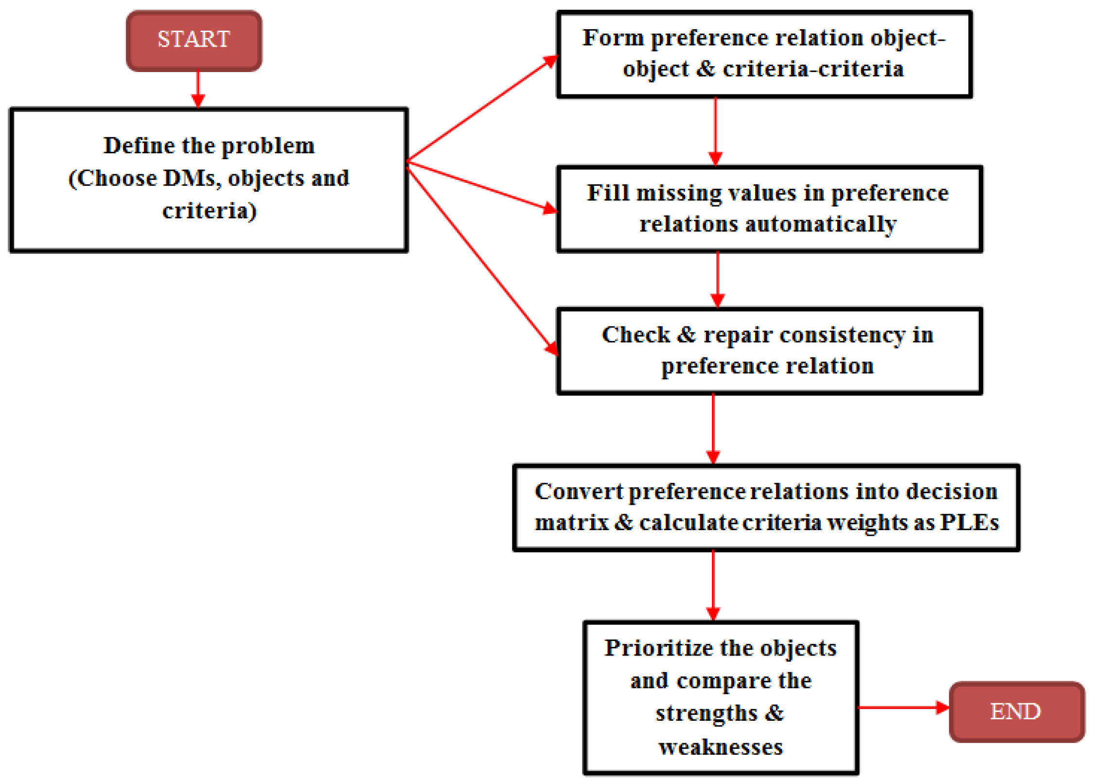
3.1. Proposed Architecture of PLPR Based Decision Framework

The architecture of the proposed scientific decision framework is presented in Figure 1 which is simple and straightforward to understand.

3.2. Proposed Automatic Procedure for Filling Missing Values and Consistency Check and Repair for PLPRs

In this section, the procedure for finding the missing values of a PLPR is presented. Generally, DMs find pairwise comparison as an easier option for rating alternatives [28]. DMs rate the alternatives upon each criterion and sometimes they are unwilling or confused between alternatives’ performance over a specific criterion and this forces them to ignore such rating. As a result, the decision matrix is now incomplete and further processing becomes difficult. To circumvent this issue, an automated procedure is proposed which automatically fits a value to the missing information. Zhang et al. [33] claimed that “(a) manual entry of missing values by some random information is unreasonable and causes potential loss of information and (b) returning of decision matrix to the DM for re-entry is also unreasonable and computationally ineffective”. Motivated by such claims, in this paper, an automated procedure is presented under PLTS context for filling missing values.
The procedure for automated filling of missing value is given below:
Step 1: Consider a PLPR R = { L i j t ( p i j t ) } n × n which has PLEs. Identify the instance which is missing. If j > i + 1 , then the missing instance can be automatically estimated (follow steps below), else follow Equation (4).
R i j = { i = 1 m r i j m , i = 1 m p i j m }   j i + 1
where r i j is the subscript of the linguistic term, p i j is the associated occurring probability of the linguistic term and m is the order of the matrix.
Step 2: When j > i + 1 , apply Equation (5) to automatically estimate the missing values.
R i j = m i n ( ( k = 1 j i 1 { r ( i + k ) ( i + k + 1 ) } ) , ( k = 1 j i 1 { r ( i + k ) ( i + k + 1 ) }     k = 1 j i 1 { ( 1 r ( i + k ) ( i + k + 1 ) ) ) } ) ) and
m i n ( ( k = 1 j i 1 { p ( i + k ) ( i + k + 1 ) } ) , ( k = 1 j i 1 { p ( i + k ) ( i + k + 1 ) }     k = 1 j i 1 { ( 1 p ( i + k ) ( i + k + 1 ) ) } ) )
where is an operator given in Definition 4.
Note 2: The result from Equation (5) is also a PLE and the values that go out of bounds when operator is applied are transformed using Remark 2.
Step 3: Check the consistency of the matrix R = ( { L i j t ( p i j t ) } ) n × n by using Equations (6) and (7).
R i j z = ( { L i j t ( p i j t ) } ) n × n
where L i j t and p i j t can be calculated by using Equation (7).
L i j t ( p i j t ) = { 1 m ( e = 1 m ( L i e ( p ) L e j ( p ) ) )   i j { s 0 }         o t h e r w i s e
where is an operator given in Definition 4.
Here linguistic terms are added as per Definition 4 and transformation procedure is applied to those terms that exceed the limits. However, the corresponding probability terms are calculated by using weighted geometry method to avoid unreasonable probability values. The personal opinion on each alternative is given by the DM with i = 1 n ω i = 1 .
Step 4: Calculate the distance between R i j and R i j z by using Equation (8) to determine the consistency index ( C I ).
C I ( R ) = d ( R i j , R i j z ) = 2 m ( m 1 ) i = 1 m j = i + 1 m ( t = 1 # L ( p ) ( p i j t × p i j t ) ( r i j t r i j t T ) ) 2
where T is the cardinality of the LTS, r is the subscript of the PLTS and p is the corresponding probability of the term set.
Note 3: The distance formula described in Equation (8) obeys the desirable distance properties viz., non-negative, non-degenerate, symmetric and transitive.
Step 5: The consistency values obtained from step 4 ( C I ( R ) ) are compared with the standard consistency value ( C I ˜ ( R ) ) (suggested as 0.05 by DMs). If C I ( R )   C I ˜ ( R ) then, R is acceptable; else R is unacceptable and automatic repairing must be done by following the steps below.
Step 6: Repair the inconsistent PLPR automatically by using Equation (9).
R i j z + 1 = ( L i j ( p ) ) 1 τ σ ( L i j ( p ) ) τ σ { ( L i j ( p ) ) 1 τ σ ( L i j ( p ) ) τ σ } { ( 1 L i j ( p ) ) 1 τ σ ( 1 L i j ( p ) ) τ σ }
where L i j ( p ) = { r i j ( p i j ) } , L i j ( p ) = { r i j ( p i j ) } , τ and σ are parameters in the range [0,1].
Note that this repairing is an iterative process and until consistent matrix is obtained, we apply the procedure.
Step 7: Repeat the steps 5 and 6 iteratively till a PLPR of acceptable consistency is obtained.

3.3. Proposed Analytic Hierarchy Process (AHP) Method under PLPR Context

Analytic hierarchy process (AHP) is a classical ranking method that is based on the pairwise comparison concept [34]. This ranking method works with preference relations and weight of each alternative is determined. Based on the weight values, alternative are ranked and the suitable object is selected for the process. Recently, Emrouznejad and Marra [35] conducted a comprehensive review on AHP method and identified its diverse applicability in MCDM and the interesting variants of AHP. Clearly from the review, extension of AHP to PLTS context is a new idea for exploration and the work of Xie et al. [32] framed the genesis for the same. Some lacunas are discussed in Section 1 which motivates the proposed extension of AHP under PLPR context.
Now, we present the procedure for ranking objects using the proposed extension to AHP under PLPR context.
Step 1: Define the problem under multi-attributes decision-making context and determine the number of objects, attributes and DMs. Use PLEs as preference information.
Step 2: Suppose, m objects and n attributes are considered, n PLPRs of order ( m × m ) is formed. Following this, a PLPR of order ( n × n ) is formed for the attributes.
Step 3: Check the consistency of all PLPRs using the procedure presented in Section 3.2 and repair the inconsistent PLPR. Apply Equation (2) to the PLPR of order ( n × n ) . This forms a weight vector for the attributes which is probabilistic linguistic in nature.
Step 4: Following step 3, we aggregate the PLEs from ( m × m ) matrices using Equation (2) to form a decision matrix with PLTS information of order ( m × n ) where m is the number of alternatives and n is the number of attributes.
Step 5: The attribute weights and decision matrix are taken from steps 3 and 4 respectively and Equation (2) is applied to obtain a vector of order ( m × 1 ) for each of the m alternatives.
Step 6: The vector obtained from step 6 contains PLTS information which is used for the final ranking by applying Equation (10).
φ i = k = 1 # L ( p ) ( r i k × p i k )
where r i is the subscript of the ith object and p i is the probability of the corresponding ith object.
Thus, the object which has large φ i value is ranked first and so on.

4. Numerical Example

4.1. Green Supplier Selection for Healthcare Center

Indian healthcare industries are gaining high interest in recent times because of its diverse spectrum of high-tech equipment, highly skilled professionals, eco-friendly infrastructure etc. On April 2015, IBEF (Indian brand equity foundation) conducted a survey and identified that Indian healthcare industries are a big asset for the nation with an outreach of USD 280 billion by 2020. The report also showed that India is ranked third in the global healthcare sector. With the motive of igniting the spirit, GoI (government of India) started many interesting and innovative initiatives (www.ibef.org) like “signing of MoA (memorandum of agreement) with WHO (world health organization) for promoting public health in India, signing MoU (memorandum of understanding) with medical agencies of BRICS to facilitate healthy medical products”. A study by Healthcare Design magazine showed that “each year, expenditure on energy usage by healthcare is USD 8 billion” which drives them to place a concrete carbon footprint. To better reduce the CO2 emission and energy usage, healthcare must tune their thoughts towards green technologies and selection of equipment suppliers who follow green standards ISO 14000 and 14001 actively.
With this train of thought, we consider a healthcare center in Tirchy that wants to expand its service and hospitality for the betterment of the people in and around the region and also reduce its contribution in carbon footprint by adopting green technology. To do so, the management decides to renovate certain policies of the hospital which include proper and hygienic service to patients, proper and effective resource management, purchase of equipment from green suppliers and intense and sensible care at critical times. Surfing through the previous reports, the management finds an urgent need to make a reasonable decision with regards to the purchase of surgical equipment for the health center. An expert committee of three members viz., chief doctor ( E 1 ) , senior stock manager ( E 2 ) and chief technical officer ( E 3 ) is formed and suitable supplier is chosen using a systematic scientific approach. Initially, seven green suppliers are chosen for the process and out of these seven suppliers four green suppliers who actively follow ISO 14000 and 14001 standards are selected based on the pre-screening test. Now, the committee decides four attributes for evaluation of four green suppliers. The committee plans to do the pairwise comparison and used PLTS information for rating. The details of these four attributes are given below:
  • Hygiene and safety ( C 1 ) : This attribute measures the amount of care given by the suppliers in adhering to the green technologies and standards.
  • Quality of equipment ( C 2 ) : The longevity and correctness of the product is determined from this attribute.
  • On-time delivery ( C 3 ) : Delivery of product at right time under critical scenario is determined from this attribute.
  • Cost of equipment ( C 4 ) : This attribute determines the total cost involved during the product life cycle.
Let us now consider the following procedure for evaluation:
Step 1: Construct four PLPRs of order ( 4 × 4 ) with PLTS information. Each criterion is taken and the DMs form pairwise comparison matrices with each supplier over a specific criterion.
The missing values in Table 1 are determined using Equation (5) and it is shown in Table 2. Clearly, the missing values which are calculated is also a PLE.
Step 2: Construct one PLPR matrix of order ( 4 × 4 ) to determine the weights of the attributes. The Equation (2) is used to determine the weight of each criterion. The weight values are probabilistic linguistic in nature.
From Table 3 we obtain the weight value (relative importance) for each criterion. By applying Equation (2) we get the weight values as PLEs and it is given by C 1 = { 2 , ( 0.32 ) , 1 , ( 0.37 ) , 2 , ( 0.41 ) } , C 2 = { 1 , ( 0.49 ) , 0 , ( 0.37 ) , 2 , ( 0.38 ) } , C 3 = { 1 , ( 0.30 ) , 1 , ( 0.32 ) , 2 , ( 0.38 ) } and C 4 = { 1 , ( 0.35 ) , 2 , ( 0.45 ) , 0 , ( 0.44 ) } .
Step 3: Check the consistency of all PLPRs and repair those PLPRs that are inconsistent in nature. Follow the procedure from Section 3.2 for automatic repairing of inconsistent PLPR.
All the above four PLPR matrices are checked for consistency by using the Equations (6) and (7). The child PLPR matrices ( R i z ) are initially formed from all four parent PLPR matrices ( R i ) and the distance between each of these PLPRs is calculated. These distance values are shown in Table 4. Just for an example, let us consider the child matrix corresponding to C 1 and the distance between the parent and child matrices are calculated and it is given in Table 4.
R 1 z = ( { 0 , ( 1 ) , 0 , ( 1 ) , 0 , ( 1 ) } { 2 , ( 0.15 ) , 0 , ( 0.14 ) , 2 , ( 0.2 ) } { 2 , ( 0.17 ) , 2 , ( 0.12 ) , 2 , ( 0.12 ) } { 2 , ( 0.17 ) , 1 , ( 0.15 ) , 2 , ( 0.15 ) } { 2 , ( 0.15 ) , 0 , ( 0.14 ) , 2 , ( 0.2 ) } { 0 , ( 1 ) , 0 , ( 1 ) , 0 , ( 1 ) } { 2 , ( 0.16 ) , 2 , ( 0.15 ) , 2 , ( 0.16 ) } { 2 , ( 0.16 ) , 1 , ( 0.18 ) , 2 , ( 0.2 ) } { 2 , ( 0.17 ) , 2 , ( 0.12 ) , 2 , ( 0.12 ) } { 2 , ( 0.16 ) , 2 , ( 0.15 ) , 2 , ( 0.16 ) } { 0 , ( 1 ) , 0 , ( 1 ) , 0 , ( 1 ) } { 2 , ( 0.18 ) , 2 , ( 0.16 ) , 2 , ( 0.12 ) } { 2 , ( 0.17 ) , 1 , ( 0.15 ) , 2 , ( 0.15 ) } { 2 , ( 0.16 ) , 1 , ( 0.18 ) , 2 , ( 0.2 ) } { 2 , ( 0.18 ) , 2 , ( 0.16 ) , 2 , ( 0.12 ) } { 0 , ( 1 ) , 0 , ( 1 ) , 0 , ( 1 ) } )
These values are compared against the standard value C I ˜ ( R ) (0.05). Since the distance values of the first three PLPRs are greater than 0.05, it is inconsistent and so we apply Equation (9) to repair these matrices. Just for an example, consider the child matrix of C 1 which becomes consistent in the second iteration with the distance value of 0.0136 which is less than the threshold 0.05. Further, child matrix of C 2 and C 3 are also inconsistent which are repaired using Equation (9) and the distance value is given by 0.018 (second iteration) and 0.019 (first iteration) which is less than the threshold value 0.05.
R 1 z + 1 = ( { 0 , ( 1 ) , 0 , ( 1 ) , 0 , ( 1 ) } { 2 , ( 0.13 ) , 0 , ( 0.12 ) , 2 , ( 0.16 ) } { 2 , ( 0.14 ) , 2 , ( 0.12 ) , 2 , ( 0.11 ) } { 2 , ( 0.14 ) , 2 , ( 0.13 ) , 2 , ( 0.13 ) } { 2 , ( 0.13 ) , 0 , ( 0.12 ) , 2 , ( 0.16 ) } { 0 , ( 1 ) , 0 , ( 1 ) , 0 , ( 1 ) } { 2 , ( 0.14 ) , 2 , ( 0.13 ) , 2 , ( 0.14 ) } { 2 , ( 0.13 ) , 1 , ( 0.15 ) , 2 , ( 0.16 ) } { 2 , ( 0.14 ) , 2 , ( 0.12 ) , 2 , ( 0.11 ) } { 2 , ( 0.14 ) , 2 , ( 0.13 ) , 2 , ( 0.14 ) } { 0 , ( 1 ) , 0 , ( 1 ) , 0 , ( 1 ) } { 2 , ( 0.15 ) , 2 , ( 0.13 ) , 2 , ( 0.1 ) } { 2 , ( 0.14 ) , 2 , ( 0.13 ) , 2 , ( 0.13 ) } { 2 , ( 0.13 ) , 1 , ( 0.15 ) , 2 , ( 0.16 ) } { 2 , ( 0.15 ) , 2 , ( 0.13 ) , 2 , ( 0.1 ) } { 0 , ( 1 ) , 0 , ( 1 ) , 0 , ( 1 ) } )
Step 4: Apply the proposed ranking method from Section 3.3 over the consistent PLPRs and obtain a suitable supplier for the process. The four PLPR matrices of order ( m × m ) and attributes weight matrix of order ( n × 1 ) are aggregated using the operator defined in Definition 4. The resultant matrix is given in Table 5.
Table 5 is formed after applying Equation (2) over the attributes-alternative pair. When Equation (2) is applied, a vector of order ( 1 × n ) is obtained for all m suppliers and finally, a decision matrix of order ( m × n ) with PLTS information is shown in Table 5. By using the procedure given in Section 3.3 on Table 5, we obtain final rank values as shown in Table 6.
From Table 6, we observe that the ranking order is given by S 1 > S 4 > S 2 > S 3 and S 1 is chosen as a suitable supplier for the healthcare. Further, suppliers S 4 , S 2 and S 3 are for backup plans. When method from [21] is applied, the ranking order becomes S 4 > S 1 > S 2 > S 3 which is different from the ranking order obtained by the proposed framework. This is evident from the fact that the method discussed in [21] does not contain occurring probability values.
Step 5: Compare the strength and weakness of the proposal with state of the art methods. Readers are encouraged to refer Section 5 for the same.

4.2. Green Supplier Selection for Automobile Industry in India

Automobile industries in India are booming at a faster pace providing economic growth and global market improvement. These industries drive avenues of employment to approximately 13 million people in India. As per the 2013–14 annual report on automobiles, a grand total of 21,500,165 vehicles were produced which eventually boomed the revenue for India. Despite the attractive advantages, the pollution caused by these industries is huge which affect the living beings and the environment as a whole. A study found that by 2020, almost half of the cars in India will use diesel and roughly 620,000 people will die due to respiratory issues (https://community.data.gov.in/automobiles-and-pollution-in-india/). This alarming analysis motivates automobile industries to choose green suppliers for purchasing their raw materials. Green suppliers actively monitor their system and practices to ensure limited emission of environmental pollutants. These suppliers strongly follow the ISO 14000 and 14001 standards pertaining to the adoption of green practices and technologies.
Motivated by this background, in this paper, we plan to provide a systematic framework for suitable selection of green supplier from the set of suppliers for leading automobile industry in India (name anonymous). Let E = ( e 1 , e 2 , e 3 ) be a set of three DMs who constitute the expert committee. G = ( g 1 , g 2 , g 3 , g 4 ) and C = ( c 1 , c 2 , c 3 , c 4 ) be the set of green suppliers and the corresponding evaluation attributes respectively. Since the attributes used in Section 4.1 adhere to the green standards, we adopt the same in this example also. Initally, eight green suppliers were chosen for the process and based on pre-screening and Delphi method, four green suppliers are finalized for evaluation. These suppliers actively obey ISO 14,000 and 14,001 standards and they are evaluated under four attributes adapted from Section 4.1. Following steps are presented for the systematic selection of green supplier:
Step 1. Form the PLPRs supplier wise for each criterion. This produces four matrices of order 4 × 4 that correspond to one preference relation for each criterion.
Step 2: Fill the missing values by using the proposed procedure given in Section 3.2. The missing values are represented by “X” in Table 7 and these values are filled systematically using procedure proposed in Section 3.2 and the values are PLEs (refer Table 8).
Step 3: Determine the consistency of each PLPR and repair the inconsistent PLPR iteratively using the proposed procedure given in Section 3.2. The d ( R 1 , R 1 z ) is 0.13 which is inconsistent and it is made consistent in two iterations with d ( R 1 , R 1 z ) as 0.013. Further, d ( R 2 , R 2 z ) is 0.091 which is inconsistent and it is made consistent in two iterations with d ( R 2 , R 2 z ) as 0.03. The d ( R 3 , R 3 z ) and d ( R 4 , R 4 z ) are 0.14 and 0.11 respectively which is inconsistent and it is made consistent with in a single iteration with d ( R 3 , R 3 z ) as 0.021 and 0.025 respectively.
R 1 z + 1 = ( { 0 , ( 1 ) , 0 , ( 1 ) , 0 , ( 1 ) } { 2 , ( 0.15 ) , 2 , ( 0.12 ) , 2 , ( 0.17 ) } { 2 , ( 0.16 ) , 2 , ( 0.13 ) , 2 , ( 0.13 ) } { 2 , ( 0.15 ) , 1 , ( 0.13 ) , 0 , ( 0.15 ) } { 2 , ( 0.15 ) , 2 , ( 0.12 ) , 2 , ( 0.17 ) } { 0 , ( 1 ) , 0 , ( 1 ) , 0 , ( 1 ) } { 2 , ( 0.16 ) , 0 , ( 0.14 ) , 0 , ( 0.16 ) } { 2 , ( 0.16 ) , 2 , ( 0.14 ) , 2 , ( 0.19 ) } { 2 , ( 0.16 ) , 2 , ( 0.13 ) , 2 , ( 0.13 ) } { 2 , ( 0.16 ) , 0 , ( 0.14 ) , 0 , ( 0.16 ) } { 0 , ( 1 ) , 0 , ( 1 ) , 0 , ( 1 ) } { 2 , ( 0.17 ) , 0 , ( 0.15 ) , 1 , ( 0.15 ) } { 2 , ( 0.15 ) , 1 , ( 0.13 ) , 0 , ( 0.15 ) } { 2 , ( 0.16 ) , 2 , ( 0.14 ) , 2 , ( 0.19 ) } { 2 , ( 0.17 ) , 0 , ( 0.15 ) , 1 , ( 0.15 ) } { 0 , ( 1 ) , 0 , ( 1 ) , 0 , ( 1 ) } )
Just as an example, the consistent PLPR R 1 ( 2 ) after second iteration is shown above.
Step 4: From step 3, we obtain consistent PLPRs which are used for prioritizing green suppliers and selection of a suitable green supplier for the automobile industry. The extended AHP under PLPR context (from Section 3.3) is used for prioritization of green suppliers.
Table 9 shows the decision matrix which is formed by applying Equation (2) over Table 8. The elements of Table 9 are PLEs and the order of the matrix is 4 × 4 .
The green suppliers are prioritized by applying Equation (2) on Table 9. Table 9 depicts the PLPR values after step 5 of Section 3.3. We again apply Equation (2) on Table 9 to obtain a vector (order 4 × 1 ) of PLEs corresponding to each green supplier. The green suppliers are prioritized using the vector and it is given by: S 1 = { 2 , ( 0.57 ) , 2 , ( 0.58 ) , 2 , ( 0.58 ) } ; S 2 = { 2 , ( 0.53 ) , 2 , ( 0.54 ) , 2 , ( 0.55 ) } ; S 3 = { 1 , ( 0.59 ) , 1 , ( 0.59 ) , 0 , ( 0.60 ) } and S 1 = { 1 , ( 0.52 ) , 0 , ( 0.53 ) , 0 , ( 0.54 ) } .
By applying Equation (10) on this vector, we obtain the ranking order as S 1 S 2 S 4 S 3 .
Step 5: Compare the superiority and weakness of the proposed framework with other methods (refer Section 5 for details).

5. Comparative Analysis: PLPR Based Decision Framework vs. Others

In this section, we make a comparative analysis of the proposed decision framework with [32] and [21]. The method [32] presents an extension to AHP method under PLTS context and method [21] extends AHP method to HFLTS context. In order to maintain homogeneity in the process of comparison, the proposed decision framework is compared with [32] and [21]. Table 10 shows the analysis of these methods under the theoretic and numeric perspectives. The theoretic factors are chosen based on intuition and the numeric factors are chosen from [36].
The strengths of the proposed decision framework are:
(1)
Unlike methods [21,27], the proposed framework can handle missing values in the PLPR in a much sensible and rational manner by automatically filling the missing values using a systematic procedure.
(2)
Though, method [27] presents a procedure for consistency check and repair, it is complex and computationally intensive as it involves Eigen vector calculation and uses logarithmic function. To circumvent the issue, the proposed framework presents a systematic procedure for consistency check and repairing inconsistent PLPRs. The procedure automatically repairs inconsistency in an iterative manner with less intervention from DMs. The proposed procedure is computationally feasible as it uses operational law(s) of PLTS.
(3)
Method [21] extends AHP under HFLTS context for ranking objects which loses potential probability information and hence, produces unreasonable ranking of objects. Further, method [27] extends AHP under PLTS context but, loses some information when transforming PLTS information to single values using possibility degree. To circumvent the issue, the proposed framework presents a method for ranking objects by extending the popular AHP under PLPR context. The preference information is retained throughout the formulation and hence, information loss is mitigated in an effective manner.
(4)
The practicality of the proposed framework is also realized by solving green supplier selection problem for a healthcare center.
(5)
Also, from the time complexity analysis, we can observe that proposed decision framework and method [27] has three crucial operations viz., (a) filling missing values, (b) check & repair of inconsistent and (c) ranking of objects with m objects and n attributes. Operation (a) takes O ( m 2 ) time complexity, operation (b) takes O ( m 2 ) time complexity and operation (c) takes O ( m 2 ( n + 1 ) ) . So, the complexity of the proposed decision framework is O ( 3 m 2 + n m 2 ) O ( m 2 ) . In contrary, the complexity of [27] (by similar analysis) is O ( m 3 + m 2 + n m 2 ) O ( m 3 ) which is evidently complex than the proposed decision framework.
Some weaknesses of the proposed framework are:
(1)
It is computationally complex because of the idea of pair-wise comparison.
(2)
Also, the agility for judgment is slow (refer Table 7) because of the pair-wise comparison.

6. Conclusions

This paper presents a new scientific decision framework under the PLPR context for rational decision-making under critical situations. The missing values are sensibly filled by using a systematic approach. Also, the consistency of the PLPR is determined and inconsistent PLPRs are repaired using the proposed method. Finally, the AHP method is extended to PLPR for selecting a suitable object from the set of objects. The practicality of the proposed decision framework is demonstrated by solving equipment supplier selection problem for a healthcare center. Also, the strengths and weaknesses of the proposal are realized by comparison with other methods under both theoretic and numeric perspectives.
Some managerial implications are presented in a nutshell below:
(1)
The proposed framework can be used as a “ready-to-use” framework for rational decision-making under uncertain situations.
(2)
Also, the consistency of the information is ensured by using a systematic procedure without loss of substantial preference information.
(3)
This framework can be used by the managers for proper planning of inventory and management of profit and risk the organization.
(4)
Further, customers can use this framework as a supplementary aid for making rational decisions.
As a part of the future scope, we plan the following research directions: (i) to present new methods for ranking under pair-wise comparison ideas; (ii) to enhance the consistency of the PLPRs under both additive and multiplicative context; (iii) to develop methods for consensus reaching by gaining motivation from [38,39] and strategic weight calculation inspired by [40,41].

Author Contributions

The individual contribution and responsibilities of the authors were as follows: R.K., K.S.R. and M.I.A. designed the research model, collected, pre-processed, and analyzed the data and the obtained results, and worked on the development of the paper. S.K. and S.K.T. provided good advice throughout the research by giving suggestions on model design, methodology, and inferences, and refined the manuscript. All the authors have read and approved the final manuscript.

Funding

This research was funded by University Grants Commission (UGC), India and Department of Science & Technology (DST), India under grant number F./2015-17/RGNF-2015-17-TAM-83 and SR/FST/ETI-349/2013.

Acknowledgments

Authors thank the editors and the anonymous reviewers for their insightful comments which improved the quality of the paper.

Conflicts of Interest

The authors declare no conflict of interest.

References

  1. Triantaphyllou, E.; Shu, B. Multi-attributes decision-making: an operations research approach. Encycl. Electr. Electron. Eng. 1998, 15, 175–186. [Google Scholar]
  2. Herrera, F.; Herrera-Viedma, E.; Verdegay, J.L. A sequential selection process in group decision-making with a linguistic assessment approach. Inf. Sci. 1995, 239, 223–239. [Google Scholar] [CrossRef]
  3. Herrera, F.; Herrera-Viedma, E.; Verdegay, J.L. Linguistic measures based on fuzzy coincidence for reaching consensus in group decision-making. Int. J. Approx. Reason. 1997, 16, 309–334. [Google Scholar] [CrossRef]
  4. Gou, X.; Xu, Z. Novel basic operational laws for linguistic terms, hesitant fuzzy linguistic term sets and probabilistic linguistic term sets. Inf. Sci. 2016, 372, 407–427. [Google Scholar] [CrossRef]
  5. Zadeh, L.A. The concept of a linguistic variable and its application to approximate reasoning–I. Inf. Sci. 1975, 8, 199–249. [Google Scholar] [CrossRef]
  6. Herrera, F.; Herrera-Viedma, E.; Verdegay, J.L. A model of consensus in group decision-making under linguistic assessments. Fuzzy Sets Syst. 1996, 78, 73–87. [Google Scholar] [CrossRef]
  7. Xu, Z. An approach based on the uncertain LOWG and induced uncertain LOWG operators to group decision-making with uncertain multiplicative linguistic preference relations. Decis. Support. Syst. 2006, 41, 488–499. [Google Scholar] [CrossRef]
  8. He, Y.; Guo, H.; Jin, M.; Ren, P. A linguistic entropy weight method and its application in linguistic multi-attribute group decision-making. Nonlinear Dyn. 2016, 84, 399–404. [Google Scholar] [CrossRef]
  9. Saaty, T.L. How to make a Decision: Analytical hierarchy process. Eur. J. Oper. Res. 1990, 48, 9–26. [Google Scholar] [CrossRef]
  10. Herrera, F.; Herrera-Viedma, E. Choice functions and mechanisms for linguistic preference relations. Eur. J. Oper. Res. 2000, 120, 144–161. [Google Scholar] [CrossRef]
  11. Herrera, F.; Herrera-Viedma, E. Linguistic decision analysis: steps for solving decision problems under linguistic information. Fuzzy Sets Syst. 2000, 115, 67–82. [Google Scholar] [CrossRef] [Green Version]
  12. Xu, Z. Deviation measures of linguistic preference relations in group decision-making. Omega 2005, 33, 249–254. [Google Scholar] [CrossRef]
  13. Morente-Molinera, J.A.; Perez, I.J.; Ureña, M.R.; Herrera-Viedma, E. Building and managing fuzzy ontologies with heterogeneous linguistic information. Knowl.-Based Syst. 2015, 88, 154–164. [Google Scholar] [CrossRef]
  14. Wang, H.; Xu, Z. Interactive algorithms for improving incomplete linguistic preference relations based on consistency measures. Appl. Soft Comput. 2016, 32, 66–79. [Google Scholar] [CrossRef]
  15. Rodriguez, R.M.; Martinez, L.; Herrera, F. Hesitant fuzzy linguistic term sets for decision-making. IEEE Trans. Fuzzy Syst. 2012, 20, 109–119. [Google Scholar] [CrossRef]
  16. Torra, V. Hesitant fuzzy sets. Int. J. Intell. Syst. 2010, 25, 529–539. [Google Scholar] [CrossRef]
  17. Zhu, B.; Xu, Z. Consistency measures for hesitant fuzzy linguistic preference relations. IEEE Trans. Fuzzy Syst. 2014, 22, 35–45. [Google Scholar] [CrossRef]
  18. Wang, H.; Xu, Z. Some consistency measures of extended hesitant fuzzy linguistic preference relations. Inf. Sci. 2015, 297, 316–331. [Google Scholar] [CrossRef]
  19. Wu, Z. A consensus process for hesitant fuzzy linguistic preference relations. In Proceedings of the 2015 IEEE International Conference on Fuzzy System, Istanbul, Turkey, 2–5 August 2015. [Google Scholar]
  20. Song, Y.; Hu, J. A group decision-making model based on incomplete comparative expressions with hesitant linguistic terms. Appl. Soft Comput. 2017, 59, 174–181. [Google Scholar] [CrossRef]
  21. Tüysüz, F.; Şimşek, B. A hesitant fuzzy linguistic term sets-based AHP approach for analyzing the performance evaluation factors: An application to cargo sector. Complex. Intell. Syst. 2017, 1–9. [Google Scholar] [CrossRef]
  22. Zhang, G.; Dong, Y.; Xu, Y. Consistency and consensus measures for linguistic preference relations based on distribution assessments. Inf. Fusion 2014, 17, 46–55. [Google Scholar] [CrossRef]
  23. Pang, Q.; Wang, H.; Xu, Z. Probabilistic linguistic term sets in multi-attribute group decision-making. Inf. Sci. 2016, 369, 128–143. [Google Scholar] [CrossRef]
  24. Zhang, B.; Liang, H.; Gao, Y.; Zhang, G. The optimization-based aggregation and consensus with minimum-cost in group decision-making under incomplete linguistic distribution context. Knowl.-Based Syst. 2018, 1–36. [Google Scholar] [CrossRef]
  25. Bai, C.; Zhang, R.; Qian, L.; Wu, Y. Comparisons of probabilistic linguistic term sets for multi-attributes decision-making. Knowl.-Based Syst. 2016, 119, 284–291. [Google Scholar] [CrossRef]
  26. Liao, H.; Jiang, L.; Xu, Z.; Xu, J.; Herrera, F. A probabilistic linguistic linear programming method in hesitant qualitative multiple attributes decision-making. Inf. Sci. 2017, 416, 341–355. [Google Scholar] [CrossRef]
  27. Liu, P.; Teng, F. Some Muirhead mean operators for probabilistic linguistic term sets and their applications to multiple attribute decision-making. Appl. Soft Comput. 2018, 68, 396–431. [Google Scholar] [CrossRef]
  28. Zhang, Y.; Xu, Z.; Wang, H.; Liao, H. Consistency-based risk assessment with probabilistic linguistic preference relation. Appl. Soft Comput. 2016, 49, 817–833. [Google Scholar] [CrossRef]
  29. Zhang, Y.; Xu, Z.; Liao, H. A consensus process for group decision-making with probabilistic linguistic preference relations. Inf. Sci. 2017, 414, 260–275. [Google Scholar] [CrossRef]
  30. Xie, W.; Ren, Z.; Xu, Z.; Wang, H. The consensus of probabilistic uncertain linguistic preference relations and the application on the virtual reality industry. Knowl.-Based Syst. 2018, 162, 14–28. [Google Scholar] [CrossRef]
  31. Wu, X.; Liao, H. A consensus-based probabilistic linguistic gained and lost dominance score method. Eur. J. Oper. Res. 2019, 272, 1017–1027. [Google Scholar] [CrossRef]
  32. Xie, W.; Xu, Z.; Ren, Z.; Wang, H. Probabilistic linguistic analytic hierarchy process and its application on the performance assessment of Xiongan new area. Int. J. Inf. Technol. Decis. Mak. 2018, 16, 1–32. [Google Scholar] [CrossRef]
  33. Liao, H.; Xu, Z.; Xia, M. Multiplicative consistency of interval-valued intuitionistic fuzzy preference relation. J. Intell. Fuzzy Syst. 2014, 27, 2969–2985. [Google Scholar]
  34. Saaty, T.L. The Analytic Hierarchy Process, 1st ed.; Mc-Graw Hill: New York, NY, USA, 1980; pp. 579–606. [Google Scholar]
  35. Emrouznejad, A.; Marra, M. The state of the art development of AHP (1979–2017): A literature review with a social network analysis. Int. J. Prod. Res. 2017, 55, 6653–6675. [Google Scholar] [CrossRef]
  36. Lima Junior, F.R.; Osiro, L.; Carpinetti, L.C.R. A comparison between Fuzzy AHP and Fuzzy TOPSIS methods to supplier selection. Appl. Soft Comput. 2014, 21, 194–209. [Google Scholar] [CrossRef]
  37. Saaty, T.L.; Ozdemir, M.S. Why the magic number seven plus or minus two. Math. Comput. Model. 2003, 28, 233–244. [Google Scholar] [CrossRef]
  38. Zhang, H.; Dong, Y.; Chen, X. The 2-rank consensus reaching model in the multigranular linguistic multiple-attribute group decision-making. IEEE Trans. Syst. Man Cybern. Syst. 2017, 48, 1–15. [Google Scholar] [CrossRef]
  39. Li, C.C.; Dong, Y.; Herrera, F. A consensus model for large-scale linguistic group decision-making with a feedback recommendation based on clustered personalized individual semantics and opposing consensus groups. IEEE Trans. Fuzzy Syst. 2018, 1–13. [Google Scholar] [CrossRef]
  40. Liu, Y.; Dong, Y.; Liang, H.; Chiclana, F.; Herrera-Viedma, E. Multiple attribute strategic weight manipulation with minimum cost in a group decision-making context with interval attribute weights information. IEEE Trans. Syst. Man Cybern. Syst. 2018, 1–12. [Google Scholar] [CrossRef]
  41. Dong, Y.; Liu, Y.; Liang, H.; Chiclana, F.; Herrera-Viedma, E. Strategic weight manipulation in multiple attribute decision-making. Omega 2018, 75, 1339–1351. [Google Scholar] [CrossRef]
Figure 1. Architecture of proposed scientific decision framework.
Symmetry 11 00002 g001
Table 1. Probabilistic Linguistic Preference Relation (PLPR) matrices for each criterion.
AttributesSupplier S 1 S 2 S 3 S 4
C 1 S 1 { 2 , ( 0.3 ) , 1 , ( 0.2 ) , 2 , ( 0.42 ) } { 2 , ( 0.33 ) , 1 , ( 0.44 ) , 1 , ( 0.2 ) } { 1 , ( 0.35 ) , 1 , ( 0.25 ) , 2 , ( 0.3 ) }
S 2 { 1 , ( 0.3 ) , 1 , ( 0.25 ) , 2 , ( 0.42 ) } { 2 , ( 0.22 ) , 1 , ( 0.4 ) , 2 , ( 0.35 ) }
S 3 { 2 , ( 0.42 ) , 2 , ( 0.25 ) , 1 , ( 0.15 ) }
S 4
C 2 S 1 { 2 , ( 0.28 ) , 1 , ( 0.35 ) , 1 , ( 0.3 ) } { 0 , ( 0.22 ) , 2 , ( 0.45 ) , 1 , ( 0.15 ) } { 2 , ( 0.18 ) , 1 , ( 0.35 ) , 1 , ( 0.25 ) }
S 2 { 2 , ( 0.4 ) , 0 , ( 0.33 ) , 1 , ( 0.25 ) } X
S 3 { 1 , ( 0.25 ) , 2 , ( 0.33 ) , 1 , ( 0.25 ) }
S 4
C 3 S 1 { 1 , ( 0.45 ) , 0 , ( 0.3 ) , 1 , ( 0.11 ) } { 2 , ( 0.25 ) , 1 , ( 0.37 ) , 1 , ( 0.33 ) } X
S 2 { 2 , ( 0.28 ) , 1 , ( 0.35 ) , 0 , ( 0.3 ) } { 1 , ( 0.35 ) , 1 , ( 0.25 ) , 2 , ( 0.3 ) }
S 3 { 2 , ( 0.33 ) , 1 , ( 0.4 ) , 2 , ( 0.22 ) }
S 4
C 4 S 1 { 1 , ( 0.3 ) , 1 , ( 0.42 ) , 2 , ( 0.25 ) } { 2 , ( 0.33 ) , 1 , ( 0.4 ) , 2 , ( 0.22 ) } { 2 , ( 0.33 ) , 0 , ( 0.35 ) , 1 , ( 0.2 ) }
S 2 { 2 , ( 0.3 ) , 2 , ( 0.24 ) , 1 , ( 0.4 ) } { 2 , ( 0.3 ) , 1 , ( 0.35 ) , 1 , ( 0.25 ) }
S 3 { 1 , ( 0.4 ) , 0 , ( 0.22 ) , 1 , ( 0.15 ) }
S 4
Table 2. PLPR matrices after finding the missing values.
AttributesSupplier S 1 S 2 S 3 S 4
C 1 S 1 { 2 , ( 0.3 ) , 1 , ( 0.2 ) , 2 , ( 0.42 ) } { 2 , ( 0.33 ) , 1 , ( 0.44 ) , 1 , ( 0.2 ) } { 1 , ( 0.35 ) , 1 , ( 0.25 ) , 2 , ( 0.3 ) }
S 2 { 1 , ( 0.3 ) , 1 , ( 0.25 ) , 2 , ( 0.42 ) } { 2 , ( 0.22 ) , 1 , ( 0.4 ) , 2 , ( 0.35 ) }
S 3 { 2 , ( 0.42 ) , 2 , ( 0.25 ) , 1 , ( 0.15 ) }
S 4
C 2 S 1 { 2 , ( 0.28 ) , 1 , ( 0.35 ) , 1 , ( 0.3 ) } { 0 , ( 0.22 ) , 2 , ( 0.45 ) , 1 , ( 0.15 ) } { 1 , ( 0.19 ) , 2 , ( 0.22 ) , 1 , ( 0.19 ) }
S 2 { 2 , ( 0.4 ) , 0 , ( 0.33 ) , 1 , ( 0.25 ) } { 2 , ( 0.4 ) , 0 , ( 0.33 ) , 1 , ( 0.25 ) }
S 3 { 1 , ( 0.25 ) , 2 , ( 0.33 ) , 1 , ( 0.25 ) }
S 4
C 3 S 1 { 1 , ( 0.45 ) , 0 , ( 0.3 ) , 1 , ( 0.11 ) } { 2 , ( 0.25 ) , 1 , ( 0.37 ) , 1 , ( 0.33 ) } { 0 , ( 0.06 ) , 0 , ( 0.08 ) , 1 , ( 0.05 ) }
S 2 { 2 , ( 0.28 ) , 1 , ( 0.35 ) , 0 , ( 0.3 ) } { 1 , ( 0.35 ) , 1 , ( 0.25 ) , 2 , ( 0.3 ) }
S 3 { 2 , ( 0.33 ) , 1 , ( 0.4 ) , 2 , ( 0.22 ) }
S 4
C 4 S 1 { 1 , ( 0.3 ) , 1 , ( 0.42 ) , 2 , ( 0.25 ) } { 2 , ( 0.33 ) , 1 , ( 0.4 ) , 2 , ( 0.22 ) } { 2 , ( 0.33 ) , 0 , ( 0.35 ) , 1 , ( 0.2 ) }
S 2 { 2 , ( 0.3 ) , 2 , ( 0.24 ) , 1 , ( 0.4 ) } { 2 , ( 0.3 ) , 1 , ( 0.35 ) , 1 , ( 0.25 ) }
S 3 { 1 , ( 0.4 ) , 0 , ( 0.22 ) , 1 , ( 0.15 ) }
S 4
Table 3. Attributes weight estimation matrix.
Attributes C 1 C 2 C 3 C 4
C 1 { 2 , ( 0.4 ) , 1 , ( 0.32 ) , 1 , ( 0.25 ) } { 1 , ( 0.25 ) , 0 , ( 0.3 ) , 1 , ( 0.35 ) } { 1 , ( 0.15 ) , 1 , ( 0.25 ) , 2 , ( 0.4 ) }
C 2 { 1 , ( 0.35 ) , 1 , ( 0.12 ) , 0 , ( 0.25 ) } { 0 , ( 0.35 ) , 2 , ( 0.32 ) , 2 , ( 0.25 ) }
C 3 { 1 , ( 0.18 ) , 1 , ( 0.4 ) , 2 , ( 0.33 ) }
C 4
Table 4. Calculation of distance values.
C I ( R ) Value(s)
d ( R 1 , R 1 z ) 0.0675
d ( R 2 , R 2 z ) 0.1267
d ( R 3 , R 3 z ) 0.0717
d ( R 4 , R 4 z ) 0.0453
Table 5. Decision matrix with probabilistic linguistic term set (PLTS) information.
Supplier vs. Attributes C 1 C 2 C 3 C 4
S 1 { 2 , ( 0.55 ) , 2 , ( 0.55 ) , 2 , ( 0.57 ) } { 2 , ( 0.56 ) , 2 , ( 0.57 ) , 2 , ( 0.53 ) } { 2 , ( 0.53 ) , 1 , ( 0.54 ) , 2 , ( 0.52 ) } { 2 , ( 0.58 ) , 2 , ( 0.62 ) , 2 , ( 0.55 ) }
S 2 { 2 , ( 0.49 ) , 2 , ( 0.51 ) , 2 , ( 0.53 ) } { 1 , ( 0.54 ) , 0 , ( 0.51 ) , 2 , ( 0.49 ) } { 2 , ( 0.51 ) , 1 , ( 0.51 ) , 2 , ( 0.51 ) } { 2 , ( 0.53 ) , 2 , ( 0.57 ) , 2 , ( 0.53 ) }
S 3 { 2 , ( 0.55 ) , 1 , ( 0.55 ) , 2 , ( 0.56 ) } { 2 , ( 0.57 ) , 2 , ( 0.57 ) , 2 , ( 0.53 ) } { 1 , ( 0.56 ) , 2 , ( 0.58 ) , 2 , ( 0.58 ) } { 2 , ( 0.59 ) , 2 , ( 0.60 ) , 0 , ( 0.56 ) }
S 4 { 2 , ( 0.49 ) , 2 , ( 0.51 ) , 2 , ( 0.52 ) } { 1 , ( 0.53 ) , 2 , ( 0.51 ) , 2 , ( 0.49 ) } { 2 , ( 0.47 ) , 2 , ( 0.48 ) , 2 , ( 0.49 ) } { 1 , ( 0.53 ) , 2 , ( 0.57 ) , 2 , ( 0.51 ) }
Table 6. Final rank values.
Supplier(s)PLTS InformationRanking Value(s)
S 1 { 2 , ( 0.56 ) , 1 , ( 0.57 ) , 2 , ( 0.54 ) } 2.7899
S 2 { 1 , ( 0.52 ) , 0 , ( 0.52 ) , 2 , ( 0.52 ) } 1.5612
S 3 { 1 , ( 0.57 ) , 1 , ( 0.58 ) , 0 , ( 0.55 ) } 1.1554
S 4 { 1 , ( 0.51 ) , 2 , ( 0.52 ) , 2 , ( 0.5 ) } 2.5677
Table 7. PLPR information supplier to supplier for each attribute.
AttributesSupplier S 1 S 2 S 3 S 4
C 1 S 1 { 3 , ( 0.35 ) , 2 , ( 0.22 ) , 2 , ( 0.40 ) } { 2 , ( 0.35 ) , 1 , ( 0.44 ) , 2 , ( 0.25 ) } { 3 , ( 0.35 ) , 2 , ( 0.25 ) , 2 , ( 0.3 ) }
S 2 { 1 , ( 0.35 ) , 2 , ( 0.3 ) , 2 , ( 0.40 ) } { 3 , ( 0.25 ) , 1 , ( 0.3 ) , 2 , ( 0.45 ) }
S 3 { 2 , ( 0.45 ) , 2 , ( 0.30 ) , 3 , ( 0.25 ) }
S 4
C 2 S 1 { 2 , ( 0.38 ) , 1 , ( 0.44 ) , 1 , ( 0.30 ) } { 0 , ( 0.25 ) , 2 , ( 0.45 ) , 1 , ( 0.45 ) } { 3 , ( 0.18 ) , 2 , ( 0.35 ) , 1 , ( 0.25 ) }
S 2 { 2 , ( 0.45 ) , 0 , ( 0.27 ) , 1 , ( 0.35 ) } X
S 3 { 1 , ( 0.25 ) , 2 , ( 0.35 ) , 1 , ( 0.35 ) }
S 4
C 3 S 1 { 1 , ( 0.45 ) , 0 , ( 0.35 ) , 2 , ( 0.18 ) } { 2 , ( 0.25 ) , 1 , ( 0.44 ) , 2 , ( 0.35 ) } X
S 2 { 2 , ( 0.42 ) , 1 , ( 0.35 ) , 0 , ( 0.35 ) } { 1 , ( 0.35 ) , 1 , ( 0.45 ) , 2 , ( 0.50 ) }
S 3 { 2 , ( 0.35 ) , 1 , ( 0.42 ) , 0 , ( 0.32 ) }
S 4
C 4 S 1 { 1 , ( 0.3 ) , 1 , ( 0.42 ) , 2 , ( 0.25 ) } { 2 , ( 0.35 ) , 1 , ( 0.42 ) , 2 , ( 0.25 ) } { 3 , ( 0.43 ) , 0 , ( 0.35 ) , 1 , ( 0.25 ) }
S 2 { 2 , ( 0.35 ) , 2 , ( 0.25 ) , 1 , ( 0.45 ) } { 2 , ( 0.4 ) , 1 , ( 0.35 ) , 3 , ( 0.25 ) }
S 3 { 2 , ( 0.45 ) , 0 , ( 0.35 ) , 1 , ( 0.25 ) }
S 4
Table 8. Filling of missing values in PLPRs.
AttributesSupplier S 1 S 2 S 3 S 4
C 1 S 1 { 3 , ( 0.35 ) , 2 , ( 0.22 ) , 2 , ( 0.40 ) } { 2 , ( 0.35 ) , 1 , ( 0.44 ) , 2 , ( 0.25 ) } { 3 , ( 0.35 ) , 2 , ( 0.25 ) , 2 , ( 0.3 ) }
S 2 { 1 , ( 0.35 ) , 2 , ( 0.3 ) , 2 , ( 0.40 ) } { 3 , ( 0.25 ) , 1 , ( 0.3 ) , 2 , ( 0.45 ) }
S 3 { 2 , ( 0.45 ) , 2 , ( 0.30 ) , 3 , ( 0.25 ) }
S 4
C 2 S 1 { 2 , ( 0.38 ) , 1 , ( 0.44 ) , 1 , ( 0.30 ) } { 0 , ( 0.25 ) , 2 , ( 0.45 ) , 1 , ( 0.45 ) } { 3 , ( 0.18 ) , 2 , ( 0.35 ) , 1 , ( 0.25 ) }
S 2 { 2 , ( 0.45 ) , 0 , ( 0.27 ) , 1 , ( 0.35 ) } { 1 , ( 0.18 ) , 1 , ( 0.23 ) , 1 , ( 0.23 ) }
S 3 { 1 , ( 0.25 ) , 2 , ( 0.35 ) , 1 , ( 0.35 ) }
S 4
C 3 S 1 { 1 , ( 0.45 ) , 0 , ( 0.35 ) , 2 , ( 0.18 ) } { 2 , ( 0.25 ) , 1 , ( 0.44 ) , 2 , ( 0.35 ) } { 0 , ( 0.11 ) , 2 , ( 0.09 ) , 0 , ( 0.08 ) }
S 2 { 2 , ( 0.42 ) , 1 , ( 0.35 ) , 0 , ( 0.35 ) } { 1 , ( 0.35 ) , 1 , ( 0.45 ) , 2 , ( 0.50 ) }
S 3 { 2 , ( 0.35 ) , 1 , ( 0.42 ) , 0 , ( 0.32 ) }
S 4
C 4 S 1 { 1 , ( 0.3 ) , 1 , ( 0.42 ) , 2 , ( 0.25 ) } { 2 , ( 0.35 ) , 1 , ( 0.42 ) , 2 , ( 0.25 ) } { 3 , ( 0.43 ) , 0 , ( 0.35 ) , 1 , ( 0.25 ) }
S 2 { 2 , ( 0.35 ) , 2 , ( 0.25 ) , 1 , ( 0.45 ) } { 2 , ( 0.4 ) , 1 , ( 0.35 ) , 3 , ( 0.25 ) }
S 3 { 2 , ( 0.45 ) , 0 , ( 0.35 ) , 1 , ( 0.25 ) }
S 4
Table 9. Decision matrix with PLTS information.
Supplier vs. Attributes C 1 C 2 C 3 C 4
S 1 { 2 , ( 0.57 ) , 2 , ( 0.56 ) , 2 , ( 0.59 ) } { 2 , ( 0.58 ) , 2 , ( 0.58 ) , 2 , ( 0.57 ) } { 2 , ( 0.55 ) , 2 , ( 0.55 ) , 2 , ( 0.55 ) } { 2 , ( 0.61 ) , 2 , ( 0.64 ) , 2 , ( 0.60 ) }
S 2 { 2 , ( 0.50 ) , 1 , ( 0.51 ) , 2 , ( 0.55 ) } { 2 , ( 0.55 ) , 1 , ( 0.52 ) , 2 , ( 0.52 ) } { 2 , ( 0.52 ) , 1 , ( 0.52 ) , 2 , ( 0.55 ) } { 2 , ( 0.54 ) , 2 , ( 0.58 ) , 2 , ( 0.60 ) }
S 3 { 2 , ( 0.56 ) , 1 , ( 0.57 ) , 2 , ( 0.58 ) } { 2 , ( 0.60 ) , 2 , ( 0.58 ) , 2 , ( 0.59 ) } { 1 , ( 0.57 ) , 1 , ( 0.59 ) , 2 , ( 0.61 ) } { 2 , ( 0.61 ) , 2 , ( 0.63 ) , 0 , ( 0.61 ) }
S 4 { 2 , ( 0.51 ) , 2 , ( 0.51 ) , 2 , ( 0.54 ) } { 1 , ( 0.53 ) , 0 , ( 0.52 ) , 2 , ( 0.51 ) } { 2 , ( 0.49 ) , 1 , ( 0.50 ) , 2 , ( 0.52 ) } { 1 , ( 0.55 ) , 2 , ( 0.59 ) , 2 , ( 0.56 ) }
Table 10. Investigation of features: Proposed vs. Others.
Context(s)Method(s)
ProposedXie et al. [32]Tuysuz and Simsek [21]
InputPLTS informationPLTS informationHFLTS information
AggregationRing sum operatorPLWGno
Weight calculationRing sum operatorEigen vectorsno
Fuzzinessyesyesyes
Occurring probabilityyesyesno
Total preorderyesyesyes
Missing value(s)Filled automatically using a systematic procedurenono
ConsistencyCheck & repair using systematic procedureCheck & repair using expectation measure for geometric consistency indexno
Adequacy testCauses rank reversal issue when adequate changes are made to objects and attributes.
ScalabilityObeys Saaty’s principle [37]
Agility ( n ( n 1 ) / 2 ) + n ( m ( m 1 ) / 2 ) where n is the number of attributes and m is the number of objects.
Ranking principlePair-wise comparison and Equation (10) are used for ranking objects.Pair-wise comparison and possibility degree measure are used for ranking objects.Pair-wise comparison and pessimistic & optimistic preference evaluation.
Information lossMitigated to a great extent by retaining the PLTS information throughout the decision processSome information is lost when PLTS information is converted into a single value using possibility degreeCrucial occurring probability value is missing in HFLTS context

