New Analytic Solutions of Queueing System for Shared–Short Lanes at Unsignalized Intersections

Abstract

Designing the crossroads capacity is a prerequisite for achieving a high level of service with the same sustainability in stochastic traffic flow. Also, modeling of crossroad capacity can influence on balancing (symmetry) of traffic flow. Loss of priority in a left turn and optimal dimensioning of shared-short line is one of the permanent problems at intersections. A shared–short lane for taking a left turn from a priority direction at unsignalized intersections with a homogenous traffic flow and heterogeneous demands is a two-phase queueing system requiring a first in–first out (FIFO) service discipline and single-server service facility. The first phase (short lane) of the system is the queueing system M(pλ)/M(μ)/1/∞, whereas the second phase (shared lane) is a system with a binomial distribution service. In this research, we explicitly derive the probability of the state of a queueing system with a short lane of a finite capacity for taking a left turn and shared lane of infinite capacity. The presented formulas are under the presumption that the system is Markovian, i.e., the vehicle arrivals in both the minor and major streams are distributed according to the Poisson law, and that the service of the vehicles is exponentially distributed. Complex recursive operations in the two-phase queueing system are explained and solved in manuscript.

1. Introduction

The initial considerations of the queuing systems for shared–short lanes at unsignalized intersections were based on the proven procedure by Harders [1], where the lengths of the short lanes are considered either as infinite or zero. In his paper, Harders had presented a limiting analytic frame of the queuing system.

Wu [2] used a pure queuing system, considering in detail the Markovian and non-Markovian systems depending on the distribution of the service, in both the steady and unsteady states of the working regimes of an unsignalized intersection. Wu noticed that the relation between the vehicles in the minor stream of a shared–short lane introduces very complex recursive operations in the queuing system, especially for left turns.

A basic problem while dimensioning shared–short Lanes is the occurrence of the “short lane domino effect” phenomena, queue overflow/short lane saturation [2] and inevitable consequences, time delay. This phenomenon is inevitable when demand exceeds its capacity. Increasing the capacity of road engineering according to Li et al. [3] has become an important way of solving traffic problems. Obligatory consequence of saturation is [4] increases in fuel consumption and [5] increased air pollution at intersections [6].

For now research on signalized intersectionsare dominant. Applying queuing theory in solutions for signalized intersections has a classic theme status and tradition longer than 60 years [7,8], with developed analytical models car-following models, macro traffic flow models, complex networks approaches, cellular automata models, traffic sensing technologies-based approaches, etc. [9]. Apart from Markovian queuing systems non-Markovian queuing systems can be found on signalized intersections [10]. Key spot in these solutions is presented in the form of shared–short Lanes for the left turn [11,12].

The solution of Shared–Short Lanes optimization for unsignalized intersections [13] is more difficult than it is for signalized intersections. Detailed explanation for different analytical approach has been given by Nielsen, Frederiksen and Simonsen [14]. Due to sequential distribution of priority, on signalized intersections deterministic solutions can be applied as well [15]. A probabilistic solution in deterministic time sequences of signalized intersection [16] and right turn solutions [17] cannot be applied for left turn. Unlike unsignalized intersections, on signalized intersections solutions can be found even under conditions of great variations of capacity [18]. One of the basic reasons is the relation between priorities [19].

A homogenous vehicle flow entering an unsignalized intersection system is characterized by simultaneous heterogeneous demands (left turn, though, and right turn). Owing to the traffic rules, the flow is separated into vehicles that are prioritized (through and right turn) and those that lose their priority (left turn). This differentiation of the flow is associated with the significant role of the binomial distribution of the arrival process. A queuing system with such specificity has been observed and explained by Yajima and Phung-Duc [20]. The previously mentioned complex recursive operations noticed by Wu [2] are based on such a binomial distribution, which determines the values and approaches to the transition between the different states of the system. Binomial distribution laws are determined on intersections as well [21] but are signalized. However binomial distribution analytically “favours” Markovian process. Poisson expression of binomial probabilities directly introduces Poisson flows into analytical tools of the queuing system, and with it exponential distribution according to the Palm theory.

The capacity of a short lane performs the spatial selection of vehicles based on the demands alters their prioritization. The basic objective is to ensure that the flow of vehicles that lose priority (left turn) according to the traffic rules do not slow down or entirely block the flow of the vehicles that retain their priority (through and right turn) owing to the first in-first out (FIFO) discipline of the service. Therefore, the proper dimensioning of a short lane has a significant effect on the capacity of the intersection and losses in time.

New analytic solutions of a Queuing system for shared–short lanes at unsignalized intersections have been presented through the following chapters after introduction:

2. Queueing system phenomenon

3. Unsignalised intersections and queueing

4. Limiting analytic framework of a queuing system

5. Calculation of the maximal number of vehicles in a system with only a shared lane

5.1. Binomial distribution of the vehicle service in a system with only a finite-capacity shared lane

5.2. Solving queuing systems with only an infinite-capacity shared lane

6. Solving a two-phase queuing system with a finite-capacity short lane i = constant and an infinite-capacity shared lane j∈[1, ∞)

6.1. Probabilities of the states of the two-phase queuing system

6.2. Validation of probability P_0,0 of a state of the two-phase queuing system

6.3. Average number of vehicle in short and share lane

7. Resultsfor maximal lane capacity of unsignalized intersection

8. Discussion

9. Conclusions

2. Queueing System Phenomenon

Queuing theory is generally considered a branch of operations research as sub-field of applied mathematics. This was founded just over 100 years ago, by the publication of works and by successful practical application by the Danish mathematician, statistician and engineer Agner Krarup Erlang (1878–1929). However, after initial success in its application, this avant-garde probabilistic methods for making decisions about the resources needed to provide a service, has provided numerous analytical limitations.

Queuing theory is based on elementary system theory, on entity structure and relations. A dominant part in queuing systems is occupied by relations—randomly distributed continuous-time. Entities are system states. They are always whole numbers and represent number of clients in the system. Based on relations between system’s intersections and systems entities, the probability of each system state is calculated.

Primary classification of queuing system depends on probabilistic distribution of time. If distribution density is exponential f(t) = λ(t)e^−λ(t), queuing system is Markovian. In case of any other time distribution, the system is non-Markovian. Markovian systems are by rule analytically available. Otherwise, if distribution density is not exponential, analytical calculation is extremely difficult and in some cases even today unsolvable. This classification has been established as an honor to Andrei Andreyevich Markov (1856–1922). David George Kendall (1918–2007) adjusted basic systematization and notation of queuing systems to primary classification.

Secondary classification has also been based on a system’s relations. If the average value of probabilistic distribution of time is constant, a queuing system is stationary. Stationary Markovian queuing system has exponential distribution density f(t) = λe^−λt, λ(t) = λ = const. The method for the analytical solution of unstationary Markovian queuing system was presented in 1931 by Nikolaevich Kolmogorov (1903–1987) [22]. Solution determined by Kolmogorov for Markovian queuing systems is principally same as for non-Markovian systems. It is based on a system of differential equations. The number of the equation is always equal to number of states, which can be infinite as well! Application of Laplace transformation for solving system of differential equation is much easier in case of Markovian queuing systems. Also, it is understood that queuing system is ergodic.

Tertiary classification is based on the use of system entity, for service and waiting. During this the queuing system can have different service disciplines: FIFO, LIFO (last in–first out), stochastic choice of service, group service, priorities in service etc. For waiting as a rule the FQFS (first in queue–first on service) discipline is used. The basic structure of the queuing system is dominantly based on tertiary classification.

Quartic classification is based on client flow. This structure can be homogenous or inhomogeneous or in other words heterogeneous. Classification has a dual nature. The simplest queuing system concept is when homogenous clients demand homogenous service. In any case of inhomogeneousness of clients and service, queuing system structure becomes delicate to solve.

Many great mathematicians and engineers had contributed to development of queuing theory: Félix Pollaczek (1892–1981) [23],Aleksandr YakovlevichKhinchin (1894–1959), our contemporary, Sir John Frank Charles Kingman (born 1939) [24], David George Kendall (1918–2007), and our other contemporary Jonh Dutton Conant Little (born 1928), etc. Their research has been dominantly pointed towards solving non-Markovian queuing systems. However, an approach towards solving nonstationary non-Markovian queuing systems has been lacking. The development of personal computers of the 1980s and 1990s made the prognosis that each queuing system could be solved by the use of simulations. This attitude has somewhat discouraged further efforts in the analytical approach of the queuing theory and was consistently described by Koenigsberg in the set and reasoned antithesis [25]. His absolutely correct assessment of the necessity of analytical approach and positive development prognosis, confirmed Schwartz, Selinka and Stoletz, especially for non-stationary time-dependent non-Markovian queuing systems [26]. The analytical approach to solving the queuing system remains an imperative. This imperative does not exist in itself, it is encouraged by the practical application of the queuing system and the lifeblood of queuing theory lies in its applications [27].

3. Unsignalised Intersections and Queueing

During the first research in the 1930s, probabilistic nature of traffic had been determined. Determined Poisson distribution in research of road infrastructure capacity in papers by Kinzer [28] and Adams [29] had for the first time proven Markovian structure of traffic flow through Conrad Palma’s (1907–1951) theorem. Whole number clients (vehicles in traffic) and exponential distribution of time between consecutive cars in free traffic flow, presented an ideal basis for the application of queuing theory. Traffic flow intensity is by rule time-dependent, or unstationary. However, dimensioning traffic infrastructure capacity of most frequent intensity or maximal intensity can be chosen and declared as stationary. This depends on the solving strategy of queuing system. This effectively expands the first two classifications.

An intersection is a queuing system. However, circumstances on intersections get extremely complicated in the parts of the third and the fourth classification. Thw parallel approach of numerous exponential flows, priority distributions, client heterogeneousness (pedestrians, cyclists, different vehicles: cars, busses, trucks, etc.), different demands (driving straight, left turn, right turn) results in a large number of interactions and complex probabilistic conditioning. Apart from this permanent imperative traffic safety, always presents additional conditions into complex probabilistic conditionality.

This conditionality is greater on unsignalized intersections. On signalized intersections in calculated time sequences, priorities are strictly distributed, which in great measure reduces probabilistic conditionality of antagonistic flows.

This paper treats intersection as Markovian stationary queuing system with FIFO service discipline, one service channel, the final capacity of short lane, endless number of places in queue/shared lane, homogenous vehicle flow with heterogeneous demands: driving straight and left turn. Demand distribution is a stationary discrete random variable of binominal distribution. Even though only one intersection segment had been considered, very complex recursive operations assumed by Wu [2], had been solved within this manuscript after 25 years.

4. Limiting Analytic Framework of a Queueing System

The probability “p” with which vehicles from the priority direction decide to make a left turn can be statistically determined based on the classic Laplacian definition of probability. It is equal to the quotient of number of vehicles turning left and total number of vehicles arriving at the intersection.

If the flow of vehicles is independent, then the Poisson flow with arbitrarily assumed average arrival rate λ can be described as two independent Poisson flows (1):

$$\lambda =p\lambda +(1-p)\lambda$$

(1)

Distribution of the service time for taking a left turn has been the subject of various analyses [30,31] starting from the first concrete application of the queueing systems to the latest research results. The approaches for the utilization of these intervals are in the domain of the time differences from minimally accepted to maximally rejected intervals of priority Poisson flow. The approximation for the service rate of a left turn as an exponential distribution of intensity μ is not very effective for a queueing system at unsignalized intersections owing to the dispersed data points. However, for the first complete analytical solution of the complex recursive operations, it is necessary to remain in the Markovian domain [12,32,33,34]. Thus, the service rate exponential distribution has been adopted here, and its derived solutions have a complete theoretical and practical relevance.

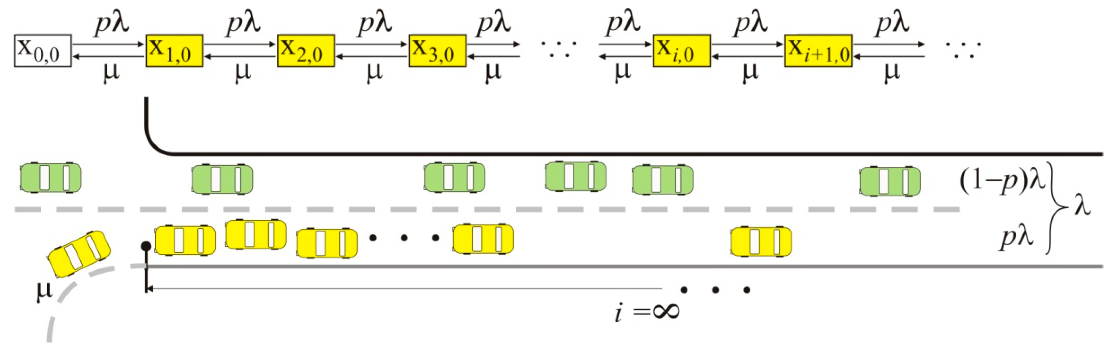
According to Harders [1], depending on the number of locations on an individual lane for taking a left turn, there are two limiting cases: minimal and maximal average number of vehicles in the system.

A minimal average number of vehicles in the system is achieved if the intersection is designed with a separate lane of unlimited capacity for taking a left turn. The vehicles that plan to move forward in the intersection have separate reserved server, and based on the priority achieve the maximal level of service. A queue is formed only by those vehicles planning to take a left turn at the intersection. In this system, average arrival rate is “pλ”and average service rate is “μ”. The discipline of the service is FIFO. There is a single server and an unlimited number of positions in the queue. This system is a classic Erlang system in which no vehicles are rejected with Kendal markings M(pλ)/M(μ)/1/∞ (Figure 1), and it has already been considered by Wu [2]. The states are determined by the number of vehicles in a separate lane for making a left turn. Accordingly, there are two indices in X_i,j, where index “i” denotes the number of vehicles in the lane for making a left turn (short lane), whereas index “j” denotes the number of locations in the lane for all the vehicles in the traffic (shared lane). In the queueing system (Figure 1), the indices of the states have values i∈[0,∞) and j = 0.

According to the formula from for queueing system with Kendal denotation M(pλ)/M(μ)/1/∞, the minimal average number of vehicles in the system is defined in (2).

$$k_{\mathit{min}}=\left(\frac{\mu -p\lambda }{\mu }\right){\displaystyle \sum _{i=0}^{\infty }i{\left(\frac{p\lambda }{\mu }\right)}^i}=\frac{p\lambda }{\mu -p\lambda }$$

(2)

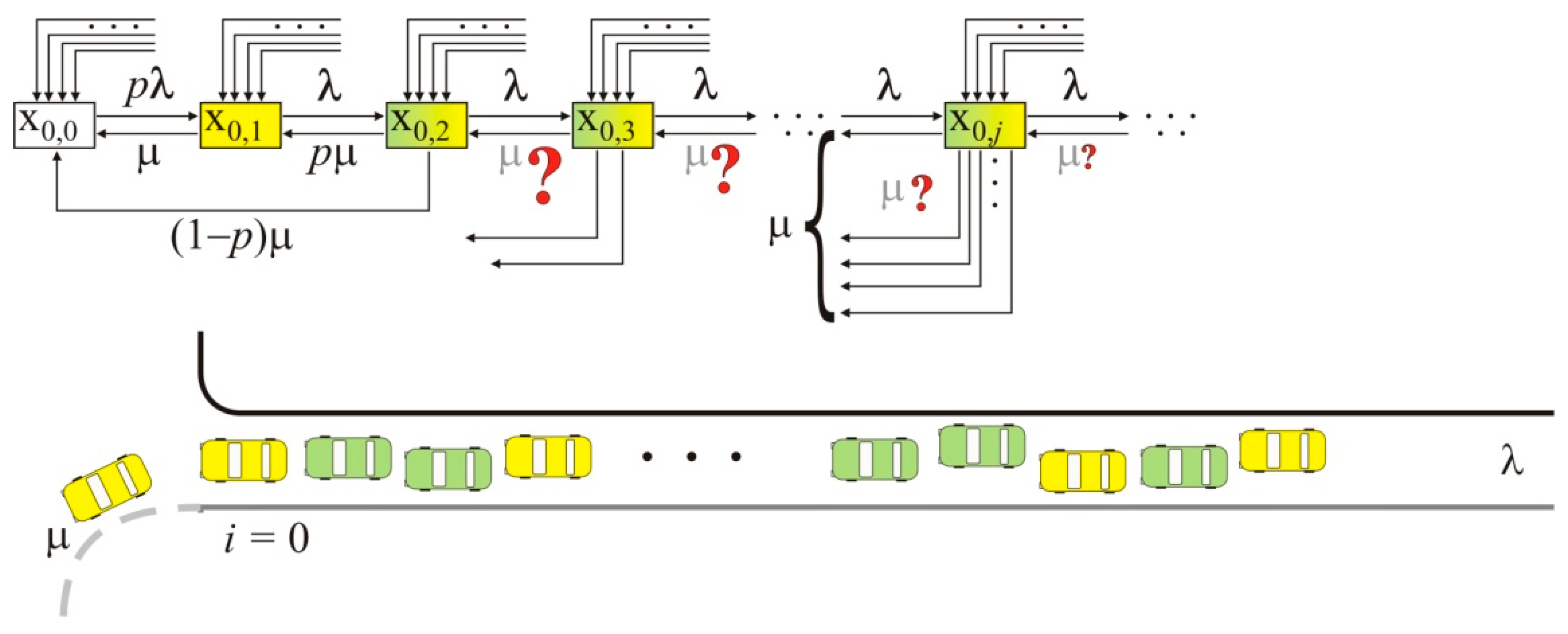
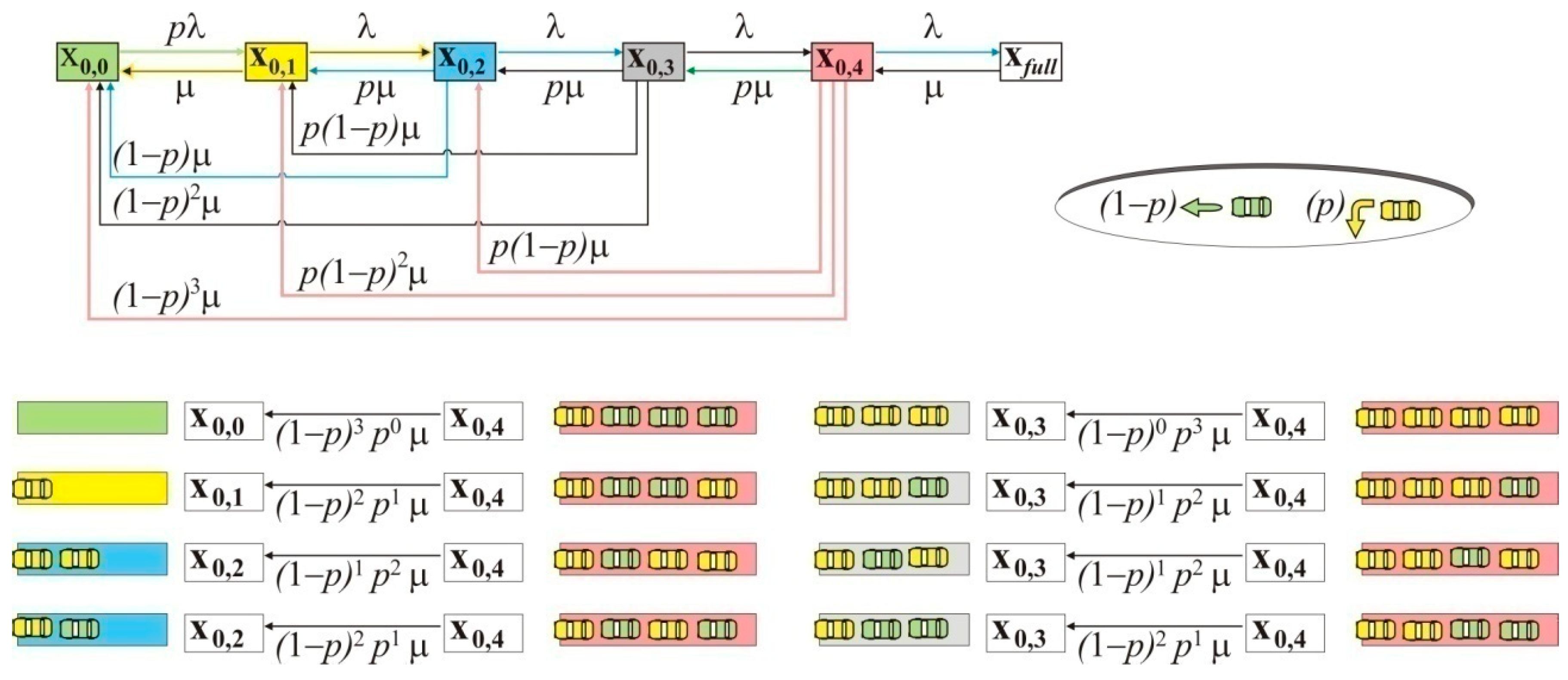
The maximal average number of vehicles in the system is achieved for all the vehicles that are present only in a single-shared lane. In the queueing system (Figure 2), the indices of the states have values i = 0 and j∈[0,∞). In this system, the arrival rate is not the same for all the states. The system crosses from state X_0,0 into state X_0,1 only on arrival of a vehicle that plans to make a left turn at the intersection with probability “p.” In this case, the arrival rate equals “pλ”. When waiting for a service owing to the FIFO discipline of the service, the server is occupied for all the other vehicles arriving at the intersection with λ intensity, and a queue is formed in the system by all the vehicles. The intensity of the service is not equal for all the states. Only the intensity of service μ from state X_0,1 is known for the vehicles performing the left-turn maneuver.

If a consecutive vehicle in state X_0,2 at the intersection plans a left−turn maneuver with probability “p”, then after servicing the vehicles from state X_0,1 in the queuing system, it switches from state X_0,2 into state X_0,1 with intensity “pμ.”

However, if a consecutive vehicle in state X_0,2 at the intersection plans to go forward with probability (1 − p), then after servicing the vehicles from state X_0,1 of the queuing system, it directly transfers from state X_0,2 to X_0,0 state with “(1− p)μ” intensity.

Depending on the binomial distribution of the vehicles, the system from state X_0,3 can transite to states X_0,2, X_0,1, or X_0,0 with different service levels. In general, the system can transite from state X_0,j into any of the previous states with different intensities, with a final summation of “μ” (Figure 2). It should be noticed that each state can be achieved from any of the following states.

The maximal average number of vehicles in this system is obtained by (3), which will be explained later in Section 5.2.

$$k_{\mathit{max}}=\frac{\mu -p\lambda }{p\left((1-p)\lambda +\mu \right)}{\displaystyle \sum _{j=0}^{\infty }j{\left(\frac{\lambda }{(1-p)\lambda +\mu }\right)}^j}=\frac{\lambda }{\mu -p\lambda }$$

(3)

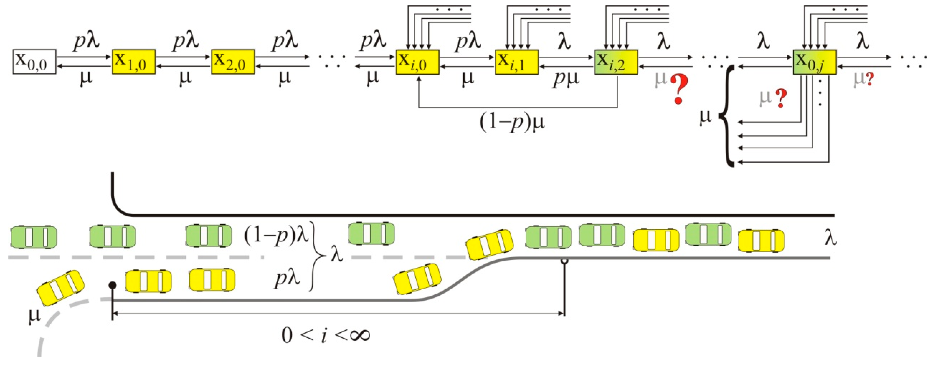
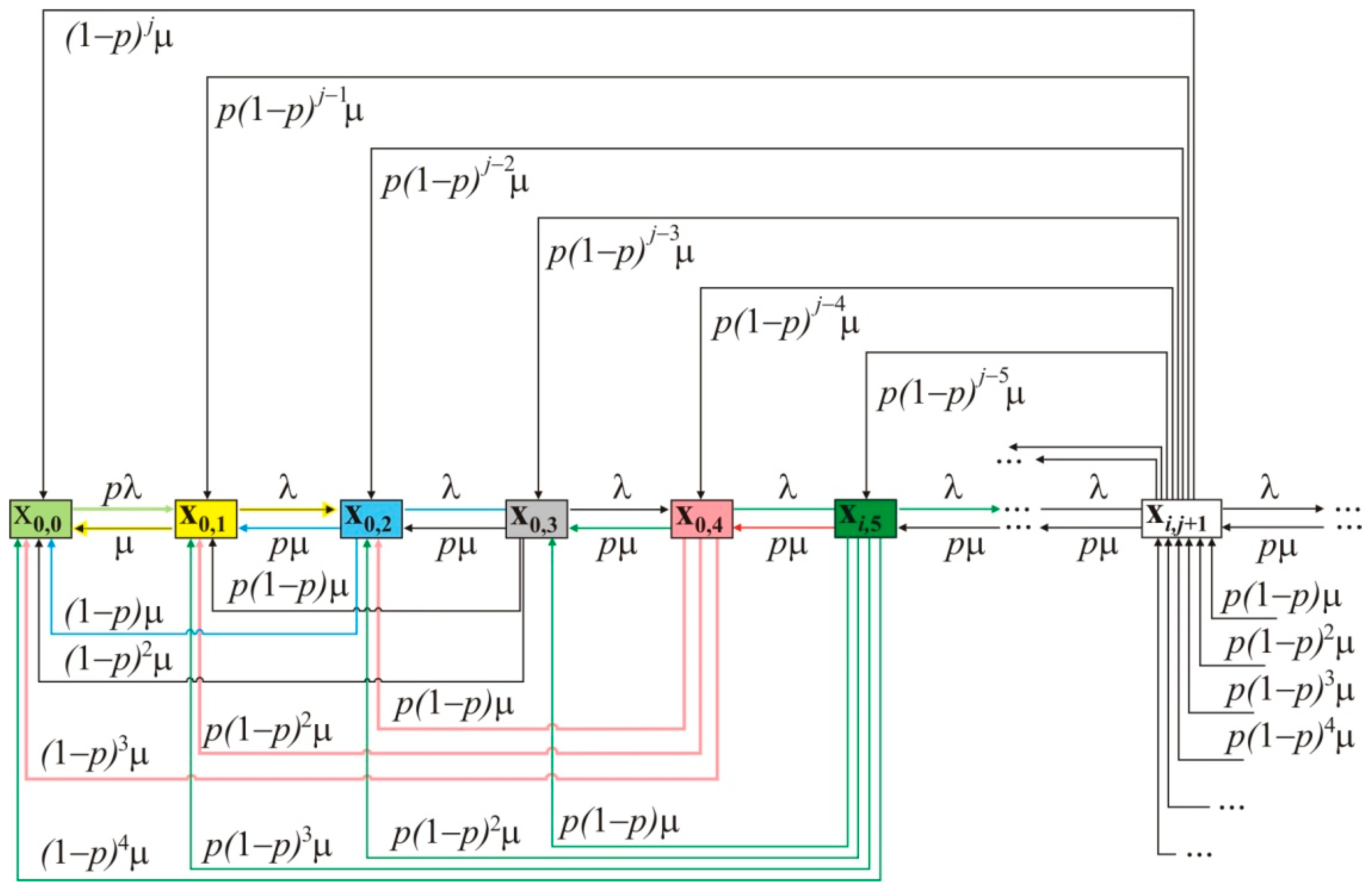
For an intersection that has a short lane designed for taking left turns with final capacity “i” and has a shared lane with unlimited number of shared places j∈[1,∞) for cars, the queueing system is presented in Figure 3.

The average number of vehicles in such a queuing system is within the limits of the minimal (2) and maximal (3). The relation between the limiting values can be obtained from expression (4).

$$k_{\mathit{min}}=\frac{p\lambda }{\mu -p\lambda }<k_i<\frac{\lambda }{\mu -p\lambda }=\frac{k_{\mathit{min}}}{p}=k_{\mathit{max}}$$

(4)

The procedure for the calculation of expression (4) will be presented in detail in Section 6.3.

The average time that a vehicle spends in this system can be calculated based on the Little formula. From Figure 3, it is obvious that this is a two-phase queueing system. The first phase corresponds to the filling of the short lane for taking left turns, from state X_0,0 to state X_i,0. State X_i,0 is the state connecting Phases I and II. The first phase finishes and the Phase II starts in the same state (X_i,0).

5. Calculation of the Maximal Number of Vehicles in a System with Only a Shared Lane

5.1. Binomial Distribution of the Vehicle Service in a System with Only a Finite-Capacity Shared Lane

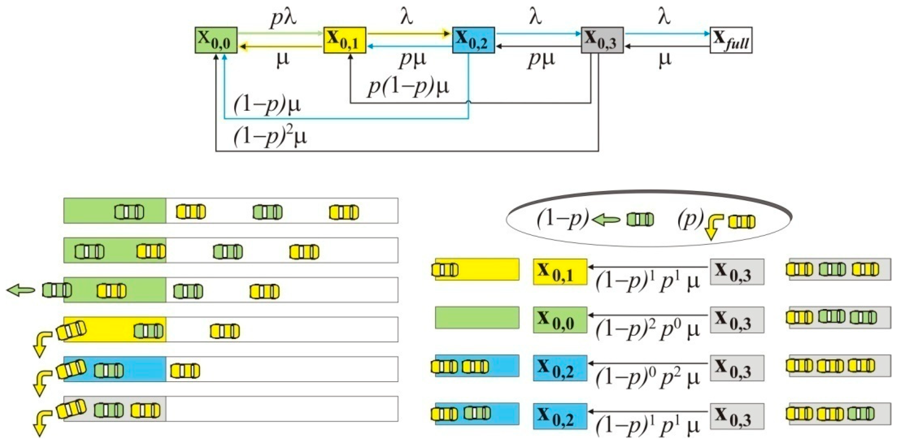
Until now we have explained the transition from state X_0,2 into X_0,0. Therefore, we next discuss the intensity of the vehicle service with capacity j = 3.

A queue in a joint lane is formed by vehicles that plan to take a left turn at the intersection with probability “p” and those vehicles that plan to drive with priority with probability “(1 − p).”

Therefore, the arrival rate is λ = pλ + (1 − p)λ (1). If the system is in state X_0,0, on arrival of a vehicle with arrival rate priority “(1 − p)λ” it will not change its state (Figure 4).

The system can only transit to state X_0,1 with the arrival of a vehicle that plans to make a left turn with arrival rate “pλ” and service intensity “μ.” This vehicle shuts down the server. Therefore, all the vehicles form a queue with arrival rate “λ.” If the system is in state X_0,1, i.e., j = 1, it can only transition into state X_0,0 with intensity of left turn μ.

If the system is in state X_0,2, it can undergo two transitions:

• into state X_0,0 with intensity “(1 − p)μ” if the second vehicle plans to drive with priority;
• into state X_0,1 with intensity “pμ” if the second vehicle in the queue plans a left-turn maneuver.
  If the system is in state X_0,3, it can make four possible transitions (Figure 4):
• into state X_0,0 with intensity “(1 − p)²μ” if the second and third vehicles plan to drive with priority;
• into state X_0,1 with intensity “(1 − p)pμ” if the second vehicle in the queue plans to driveride with priority;
• into state X_0,2 with intensity “p²μ” if both the second and third vehicles plan a left-turn maneuver;
• into the X_0,2 with intensity “(1 − p)pμ” if the second vehicle plans a left-turn maneuver whereas the third vehicle plans to drive with priority.

It should be noted that the total intensity of the transitions into state X_0,2 is p²μ + (1 − p)pμ = pμ.

It can be generalized that from each state X_0,j, there are 2^j−1 possible transitions to each of the previous states. The balance (differential) equations of the steady-states are expressed in (5).

$$\begin{array}{l}{P^{\prime }}_{0,0}(t)=0=-\lambda p{P}_{0,0}+\mu P_{0,1}+(1-p)\mu P_{0,2}+(1-p{)}^2\mu P_{0,3}\\ {P^{\prime }}_{0,1}(t)=0=+\lambda p{P}_{0,0}-\lambda P_{0,1}-\mu P_{0,1}+p\mu P_{0,2}+p(1-p)\mu P_{0,3}\\ {P^{\prime }}_{0,2}(t)=0=+\lambda P_{0,1}-\lambda P_{0,2}-p\mu P_{0,2}-(1-p)\mu P_{0,2}+p\mu P_{0,3}\\ {P^{\prime }}_{0,3}(t)=0=+\lambda P_{0,2}-p\mu P_{0,3}-(1-p)p\mu P_{0,3}-(1-p{)}^2\mu P_{0,3}+\mu P_{full}\\ {P^{\prime }}_{full}(t)=0=+\lambda P_{0,3}-\mu P_{full}\end{array}\}$$

(5)

To observe the binomial laws, a system with capacity j = 4 is also considered (Figure 5).

The balance (differential) equations of the steady-state of the queueing system with four places in the queue for vehicles in a joint traffic lane are given in (6).

$$\begin{array}{l}{P^{\prime }}_{0,0}(t)=0=-\lambda p{P}_{0,0}+\mu P_{0,1}+(1-p{)}^1\mu P_{0,2}+(1-p{)}^2\mu P_{0,3}+(1-p{)}^3\mu P_{0,4}\\ {P^{\prime }}_{0,1}(t)=0=+\lambda p{P}_{0,0}-\lambda P_{0,1}-\mu P_{0,1}+p\mu P_{0,2}+p(1-p)\mu P_{0,3}+p(1-p{)}^2\mu P_{0,4}\\ {P^{\prime }}_{0,2}(t)=0=+\lambda P_{0,1}-\lambda P_{0,2}-p\mu P_{0,2}+(1-p)\mu P_{0,2}+p\mu P_{0,3}+p(1-p)\mu P_{0,4}\\ {P^{\prime }}_{0,3}(t)=0=+\lambda P_{0,2}-P_{0,3}(\lambda +p\mu +p\mu (1-p)+\mu (1-p{)}^2)+p\mu P_{0,4}\\ {P^{\prime }}_{0,4}(t)=0=+\lambda P_{0,3}-P_{0,4}(\lambda +p\mu +p\mu (1-p)+p\mu {(1-p)}^2+\mu {(1-p)}^3)+\mu P_{full}\\ {P^{\prime }}_{full}(t)=0=+\lambda P_{0,4}-\mu P_{full}\end{array}\}$$

(6)

The system can switch from state X_0,4 into state X_0,3 in four ways, which are included in the binomial expression in (7).

$$\mu \left(p^3{(1-p)}^0+2p^2{(1-p)}^1+p^1{(1-p)}^2\right)=p\mu {\displaystyle \sum _{k=0}^2\left(\begin{array}{c}2\\ k\end{array}\right)p^k{(1-p)}^{2-k}}$$

(7)

From each X_0,j state there are (j − 2) ways to switch to X_0,j−1 state, which are included in the binomial expression for complementary probabilities, as expressed in (8):

$$p\mu {\displaystyle \sum _{k=0}^{j-2}\left(\begin{array}{c}j-2\\ k\end{array}\right)p^k{(1-p)}^{j-2-k}=}p\mu {\left(p+(1-p)\right)}^{j-2}=p\mu {\left(1\right)}^{j-2}=p\mu$$

(8)

and there are (n − 1) ways to switch from each states X_{0,j∈[2, ∞]} to state X_{0,n∈[1, j−1]}, which are included in the binomial expression of complementary probabilities given in (9), for k∈N.

$$p{(1-p)}^{j-n-1}\mu {\displaystyle \sum _{k=0}^{n-1}\left(\begin{array}{c}n-1\\ k\end{array}\right)p^k{(1-p)}^{n-1-k}=}p\mu {\left(p+(1-p)\right)}^{n-2}=p{(1-p)}^{j-n-1}\mu$$

(9)

The exception is state X_0,0 whose intensities are expressed as the product of the probabilities of each state in a geometric series (10).

$$\mu {\displaystyle \sum _{j=0}^{\infty }{(1-p)}^j}{P}_{0,j}$$

(10)

From each state j∈[1, k], k∈N, intensity of the vehicle service “μ” “spills” according to the partial geometric dependence defined in (11).

$$\mu {(1-p)}^{j-1}+p\mu {\displaystyle \sum _{k=0}^{j-2}{(1-p)}^k}+=\mu {(1-p)}^{j-1}+p\mu \frac{1-{(1-p)}^{j-1}}{1-(1-p)}=\mu$$

(11)

5.2. Solving Queueing Systems with Only an Infinite-Capacity Shared Lane

A queueing system in which no vehicles are rejected, because of the absence of a short lane (i = 0), in a heterogeneous vehicle flow with an infinite-capacity shared lane has states as presented in Figure 6.

The system of balance equations of the corresponding steady-state is given in (12), k∈N.

$$\begin{array}{l}{P^{\prime }}_{0,0}(t)=0=-p\lambda P_{0,0}+\frac{1}{p}{\displaystyle \sum _{j=1}^{\infty }p{(1-p)}^{j-1}\mu P_{0,j}}\\ {P^{\prime }}_{0,1}(t)=0=p\lambda P_{0,0}-(\lambda +\mu )P_{0,1}+{\displaystyle \sum _{j=2}^{\infty }p{(1-p)}^{j-2}\mu P_{0,j}}\\ {P^{\prime }}_{0,2}(t)=0=\lambda P_{0,1}-(\lambda +\mu )P_{0,2}+{\displaystyle \sum _{j=3}^{\infty }p{(1-p)}^{j-3}\mu P_{0,j}}\\ \dots \\ {P^{\prime }}_{0,k+1}(t)=0=\lambda P_{0,k}-(\lambda +\mu )P_{0,k+1}+{\displaystyle \sum _{j=k+2}^{\infty }p{(1-p)}^{j-(k+2)}\mu P_{0,j}}\\ \dots \end{array}\}$$

(12)

From the balance equations of the steady-state of the system in (12), the relations between the probabilities and sums of the series of the geometric products of the probabilities are obtained, as given in (13).

$$\begin{array}{l}p\lambda P_{0,0}=\frac{1}{p}{\displaystyle \sum _{j=1}^{\infty }p{(1-p)}^{j-1}\mu P_{0,j}}\\ (\lambda +\mu )P_{0,1}-\lambda P_{0,0}={\displaystyle \sum _{j=2}^{\infty }p{(1-p)}^{j-2}\mu P_{0,j}}\\ (\lambda +\mu )P_{0,2}-\lambda P_{0,1}={\displaystyle \sum _{j=3}^{\infty }p{(1-p)}^{j-3}\mu P_{0,j}}\\ \dots \\ (\lambda +\mu )P_{0,k}-\lambda P_{0,k-1}={\displaystyle \sum _{j=k+1}^{\infty }p{(1-p)}^{j-k-1}\mu P_{0,j}}\\ \dots \end{array}\}$$

(13)

The relations between the sums should be noticed (14).

$$\begin{array}{l}{\displaystyle \sum _{j=1}^{\infty }p{(1-p)}^{j-1}\mu P_j}=p\mu P_{0,1}+(1-p){\displaystyle \sum _{j=2}^{\infty }p{(1-p)}^{j-2}\mu P_{0,j}}\\ {\displaystyle \sum _{j=2}^{\infty }p{(1-p)}^{n-2}\mu P_{0,j}}=p\mu P_{0,2}+(1-p){\displaystyle \sum _{j=3}^{\infty }p{(1-p)}^{j-3}\mu P_{0,j}}\\ {\displaystyle \sum _{j=3}^{\infty }p{(1-p)}^{n-3}\mu P_{0,j}}=p\mu P_{0,3}+(1-p){\displaystyle \sum _{j=4}^{\infty }p{(1-p)}^{j-4}\mu P_{0,j}}\\ \dots \\ {\displaystyle \sum _{j=k}^{\infty }p{(1-p)}^{j-k}\mu P_{0,j}}=p\mu P_{0,k}+(1-p){\displaystyle \sum _{j=k+1}^{\infty }p{(1-p)}^{j-(k+1)}\mu P_{0,j}}\\ \dots \end{array}\}$$

(14)

From the first balance equation of the steady-state in (12), expression (15) can be obtained.

$$p\lambda P_{0,0}=\frac{1}{p}{\displaystyle \sum _{j=1}^{\infty }p{(1-p)}^{j-1}\mu P_{0,j}}\iff p^2\lambda P_{0,0}=p\mu P_{0,1}+(1-p){\displaystyle \sum _{j=2}^{\infty }p{(1-p)}^{j-2}\mu P_{0,j}}$$

(15)

From the second relation of the sums in (14), we can obtain expression (16).

$$\begin{array}{c}{p}^2\lambda P_{0,0}=p\mu P_{0,1}+(1-p)\left[(\lambda +\mu )P_{0,1}-p\lambda P_{0,0}\right]\\ p\lambda P_{0,0}=\lambda P_{0,1}+\mu P_{0,1}-p\lambda P_{0,1}\iff P_{0,1}=\frac{p\lambda }{(1-p)\lambda +\mu }{P}_{0,0}\end{array}$$

(16)

From the second balance equation in (12) of the steady-state, expression (17) can be obtained.

$$(\lambda +\mu )P_{0,1}-p\lambda P_{0,0}=p\mu P_{0,2}+(1-p){\displaystyle \sum _{j=3}^{\infty }p{(1-p)}^{j-3}\mu P_{0,j}}$$

(17)

From the third relation of the sums in (14), expression (18) can be derived.

$$\begin{array}{c}(\lambda +\mu )P_{0,1}-p\lambda P_{0,0}=p\mu P_{0,2}+(1-p)\left[(\lambda +\mu )P_{0,2}-\lambda P_{0,1}\right]\\ \left[(1-p)\lambda +\mu \right]P_{0,2}=\frac{\left[2\lambda -p\lambda +\mu \right]-\left[\lambda -p\lambda +\mu \right]}{(1-p)\lambda +\mu }p\lambda P_{0,0}\iff P_{0,2}=\frac{p{\lambda }^2{P}_{0,0}}{{\left[(1-p)\lambda +\mu \right]}^2}\end{array}$$

(18)

Furthermore, from the third balance equation of the steady-state of the system, expression (19) can be obtained.

$$(\lambda +\mu )P_{0,2}-\lambda P_1={\displaystyle \sum _{j=3}^{\infty }p{(1-p)}^{j-3}\mu P_{0,j}}=p\mu P_{0,3}+(1-p){\displaystyle \sum _{j=4}^{\infty }p{(1-p)}^{j-4}\mu P_{0,j}}$$

(19)

From the fourth relation of the sums, expression (20) can be obtained.

$$\begin{array}{c}(\lambda +\mu )P_{0,2}-\lambda P_1=p\mu P_{0,3}+(1-p)\left[(\lambda +\mu )P_{0,3}-\lambda P_{0,2}\right]\\ \left[(1-p)\lambda +\mu \right]P_{0,3}=\left[(2-p)\lambda +\mu \right]P_{0,2}-\lambda P_{0,1}\iff P_{0,3}=\frac{p{\lambda }^3{P}_{0,0}}{{\left[(1-p)\lambda +\mu \right]}^3}\end{array}$$

(20)

From (16), (18) and (20) the recurrent relation for the probabilities of the states, P_0,j is obtained analogously (21), and can be proved by mathematical induction.

$$P_{0,j}=\frac{p{\lambda }^j{P}_{0,0}}{{\left[(1-p)\lambda +\mu \right]}^j}$$

(21)

From the condition in (22):

$$P_{0,0}+P_{0,1}+P_{0,2}+\dots ={\displaystyle \sum _{j=0}^{\infty }{P}_{0,j}}$$

(22)

The probability of the initial state in (23) is obtained. Under the stability condition μ ≥ p λ and 0 ≤ p ≤ 1, probability of the state without a vehicle is always 0 ≤ P_0,0 ≤ 1.

$$P_{0,0}=\frac{1}{p{\displaystyle \sum _{j=0}^{\infty }{\left(\frac{\lambda }{(1-p)\lambda +\mu }\right)}^j}}=\frac{1}{p}\left(1-\frac{\lambda }{(1-p)\lambda +\mu }\right)=\frac{\mu -p\lambda }{p\left((1-p)\lambda +\mu \right)}$$

(23)

From the recurrent relation of the probabilities of the states for i = 0 and j∈[0, ∞), (24) is obtained.

$$P_{0,j}=\frac{\mu -p\lambda }{p\left((1-p)\lambda +\mu \right)}\frac{p{\lambda }^j}{{\left[(1-p)\lambda +\mu \right]}^j}=\frac{\mu -p\lambda }{\left((1-p)\lambda +\mu \right)}\frac{{\lambda }^j}{{\left[(1-p)\lambda +\mu \right]}^j}$$

(24)

The average number of vehicles in the system is defined in (25)

$$k_{\mathit{max}}={\displaystyle \sum _{j=0}^{\infty }k{P}_{0,j}}=\frac{\frac{\mu -p\lambda }{(1-p)\lambda +\mu }}{1-\frac{\mu -p\lambda }{(1-p)\lambda +\mu }}=\frac{\lambda }{\mu -p\lambda }$$

(25)

This average number of vehicles is the maximal average number of vehicles k_max in (2) achieved in the queueing system for the given values of λ, μ, and p. It is obvious that when pλ = μ, the average number of vehicles diverges, and under the stability condition μ ≥ pλ, the system does not fulfill its objective (26).

$$\underset{p\lambda \to \mu }{\mathit{lim}}{k}_{\mathit{max}}=\underset{p\lambda \to \mu }{\mathit{lim}}\frac{\lambda }{\mu -p\lambda }=\infty$$

(26)

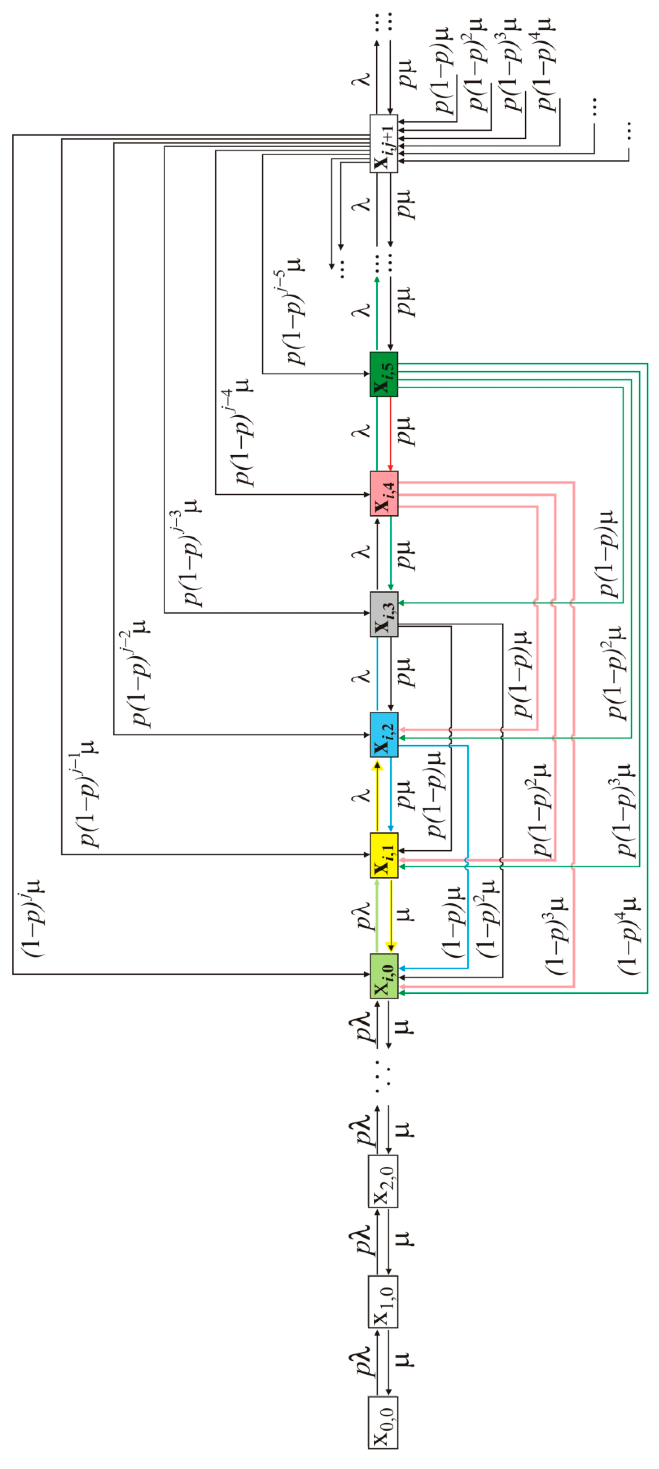
6. Solving a Two-Phase Queueing System with a Finite-Capacity Short Lane i=Const and an Infinite-Capacity Shared Lane j∈[1, ∞)

This queueing system is the usual state in practical conditions. The system has one server for taking a left turn. A separate lane for the left turn is designed, and it has finite capacity “i”. A separate lane fills with a homogenous vehicle flow with a homogenous demand that becomes a heterogeneous demandon at unsignalized intersections when vehicles plan a left-turn maneuver. If product “pλ”converges to service rate “μ” or if there is high participation of “p” in the incoming flow, vehicles fill all the places “i” in the short lane, and then form a queue of heterogeneous vehicles in the shared lane with intensity “λ.” The graph of the states of the queueing system is presented in Figure 7.

6.1. Probabilities of the States of the Two-Phase Queueing System

The connecting phases I and II is state P_i,0. The balance equations of the steady-state of the two-phase system are given in (27).

$$\begin{array}{l}{P^{\prime }}_{0,0}(t)=0=-p\lambda P_{0,0}+\mu P_{1,0}\\ {P^{\prime }}_{1,0}(t)=0=+p\lambda P_{0,0}-p\lambda P_{1,0}-\mu P_{1,0}+\mu P_{2,0}\\ \\ \dots \\ {P^{\prime }}_{i-1,0}(t)=0=+p\lambda P_{i-2,0}-p\lambda P_{i-1,0}-\mu P_{i-1,0}+\mu P_{i,0}\\ {P^{\prime }}_{i,0}(t)=0=+p\lambda P_{i-1,0}-p\lambda P_{i,0}-\mu P_{i,0}+\frac{1}{p}{\displaystyle \sum _{j=1}^{\infty }p{(1-p)}^{j-1}\mu P_{i,j}}\\ {P^{\prime }}_{i,1}(t)=0=\lambda P_{i,0}-(\lambda +\mu )P_{i,1}+{\displaystyle \sum _{j=2}^{\infty }p{(1-p)}^{j-2}\mu P_{i,j}}\\ {P^{\prime }}_{i,2}(t)=0=\lambda P_{i,1}-(\lambda +\mu )P_{i,2}+{\displaystyle \sum _{j=3}^{\infty }p{(1-p)}^{j-3}\mu P_{i,j}}\\ {P^{\prime }}_{i,3}(t)=0=\lambda P_{i,2}-(\lambda +\mu )P_{i,3}+{\displaystyle \sum _{j=4}^{\infty }p{(1-p)}^{j-4}\mu P_{i,j}}\\ \mathrm{....}\end{array}\}$$

(27)

From state X_0,0 to state X_i,0, there are known relations based on the system M(pλ)/M(μ)/i/∞ (28).

$$\begin{array}{l}p\lambda P_{0,0}=\mu P_{1,0}\iff P_{1,0}=\frac{p\lambda }{\mu }{P}_{0,0}\\ \lambda \frac{p\lambda }{\mu }{P}_{0,0}+\mu \frac{p\lambda }{\mu }{P}_{0,0}-p\lambda P_{0,0}=\mu P_{2,0}\iff P_{2,0}={\left(\frac{p\lambda }{\mu }\right)}^2{P}_{0,0}\\ P_{3,0}={\left(\frac{p\lambda }{\mu }\right)}^3{P}_{0,0}\\ \dots \\ P_{i-1,0}={\left(\frac{p\lambda }{\mu }\right)}^{i-1}{P}_{0,0}\\ P_{i,0}=\frac{p\lambda }{\mu }{P}_{i-1,0}={\left(\frac{p\lambda }{\mu }\right)}^i{P}_{0,0}\end{array}\}$$

(28)

For further solving the new relations between the sums, the expressions in (29) need to be noted (k∈N).

$$\begin{array}{l}{\displaystyle \sum _{j=1}^{\infty }p{(1-p)}^{j-1}\mu P_{i,j}}=p\mu P_{i,1}+(1-p){\displaystyle \sum _{j=2}^{\infty }p{(1-p)}^{j-2}\mu P_{i,j}}\\ {\displaystyle \sum _{j=2}^{\infty }p{(1-p)}^{j-2}\mu P_{i,j}}=p\mu P_{i,2}+(1-p){\displaystyle \sum _{j=3}^{\infty }p{(1-p)}^{j-3}\mu P_{i,j}}\\ {\displaystyle \sum _{j=3}^{\infty }p{(1-p)}^{j-3}\mu P_{i,j}}=p\mu P_{i,3}+(1-p){\displaystyle \sum _{j=4}^{\infty }p{(1-p)}^{j-4}\mu P_{i,j}}\\ \dots \\ {\displaystyle \sum _{j=k}^{\infty }p{(1-p)}^{j-k}\mu P_{i,k}}=p\mu P_{i,k}+(1-p){\displaystyle \sum _{j=k+1}^{\infty }p{(1-p)}^{j-(k+1)}\mu P_{i,j}}\\ \dots \end{array}\}$$

(29)

From the equation for P_i,1, by changing the sum for j = 3, (30) is obtained.

$$\begin{array}{c}(\lambda +\mu )P_{i,1}-\lambda P_{i,0}={\displaystyle \sum _{j=2}^{\infty }p{(1-p)}^{j-2}\mu P_{i,j}}\\ (\lambda +\mu )P_{i,1}-\lambda P_{i,0}=p\mu P_{i,2}+(1-p){\displaystyle \sum _{j=3}^{\infty }p{(1-p)}^{j-3}\mu P_{i,j}}\\ (\lambda +\mu )P_{i,1}-\lambda P_{i,0}=p\mu P_{i,2}-(1-p)\left(\lambda P_{i,1}-(\lambda +\mu )P_{i,2}\right)\\ \left[(2-p)\lambda +\mu \right]P_{i,1}-\lambda P_{i,0}=\left[(1-p)\lambda +\mu \right]P_{i,2}\iff \lambda P_{i,0}=\left[(2-p)\lambda +\mu \right]P_{i,1}-\left[(1-p)\lambda +\mu \right]P_{i,2}\\ P_{i,0}=\left[(2-p)+\frac{\mu }{\lambda }\right]P_{i,1}-\left[(1-p)+\frac{\mu }{\lambda }\right]P_{i,2}\end{array}$$

(30)

From the equation for P_i,2, by changing the sum for j = 4, (31) is obtained.

$$\begin{array}{c}(\lambda +\mu )P_{i,2}-\lambda P_{i,1}={\displaystyle \sum _{j=3}^{\infty }p{(1-p)}^{j-3}\mu P_{i,j}}\\ (\lambda +\mu )P_{i,2}-\lambda P_{i,1}=p\mu P_{i,3}+(1-p){\displaystyle \sum _{j=4}^{\infty }p{(1-p)}^{j-4}\mu P_{i,j}}\\ (\lambda +\mu )P_{i,2}-\lambda P_{i,1}=p\mu P_{i,3}-(1-p)\left(\lambda P_{i,2}-(\lambda +\mu )P_{i,3}\right)\\ \left[(2-p)\lambda +\mu \right]P_{i,2}-\lambda P_{i,1}=\left[(1-p)\lambda +\mu \right]P_{i,3}\\ P_{i,1}=\left[(2-p)+\frac{\mu }{\lambda }\right]P_{i,2}-\left[(1-p)+\frac{\mu }{\lambda }\right]P_{i,3}\end{array}$$

(31)

Furthermore, a recurrent relation given in (32) is obtained.

$$P_{i,k}=\left[(2-p)+\frac{\mu }{\lambda }\right]P_{i,k+1}-\left[(1-p)+\frac{\mu }{\lambda }\right]P_{i,k+2}$$

(32)

From the normative condition in (33):

$${\displaystyle \sum _{k=0}^{i-1}{P}_{k,0}}+{\displaystyle \sum _{j=0}^{\infty }{P}_{i,j}}=\left(P_{0,0}+P_{1,0}+\dots +P_{i-1,0}\right)+\left(P_{i,0}+P_{i,1}+P_{i,2}+P_{i,3}\dots \right)=1$$

(33)

and applying the recurrent equation in (32), (34) can be derived.

$$\begin{array}{l}{\displaystyle \sum _{k=0}^{i-1}{P}_{k,0}}+\left[(2-p)+\frac{\mu }{\lambda }\right]P_{i,1}\underset{P_{i,2}}{\underbrace{-\left[(1-p)+\frac{\mu }{\lambda }\right]P_{i,2}+\left[(2-p)+\frac{\mu }{\lambda }\right]P_{i,2}}}\\ \underset{P_{i,3}}{\underbrace{-\left[(1-p)+\frac{\mu }{\lambda }\right]P_{i,3}+\left[(2-p)+\frac{\mu }{\lambda }\right]P_{i,3}}}\underset{{\mathrm{P}}_{\mathrm{i},4}}{\underbrace{-\left[(1-p)+\frac{\mu }{\lambda }\right]P_{i,4}+\dots }}=1\end{array}$$

(34)

Then the normative condition becomes (35).

$${\displaystyle \sum _{k=0}^{i-1}{P}_{k,0}}+\left[(2-p)+\frac{\mu }{\lambda }\right]P_{i,1}+P_{i,2}+P_{i,3}+\dots =1$$

(35)

Since,

$$\left[(2-p)+\frac{\mu }{\lambda }\right]P_{i,1}=2P_{i,1}-p{P}_{i,1}+\frac{\mu }{\lambda }{P}_{i,1}=\left[(1-p)+\frac{\mu }{\lambda }\right]P_{i,1}+P_{i,1}$$

(36)

The normative condition can be given as (37).

$${\displaystyle \sum _{k=0}^{i-1}{P}_{k,0}}+\left[(1-p)+\frac{\mu }{\lambda }\right]P_{i,1}+P_{i,1}+P_{i,2}+\dots =1$$

(37)

By expanding (37) with (±P_i,0), the direct relation between probabilities P_i,0 and P_i,1 is obtained from the normative condition, and it is given in (38).

$${\displaystyle \sum _{k=0}^{i-1}{P}_{k,0}}+\left[(1-p)+\frac{\mu }{\lambda }\right]P_{i,1}+(-P_{i,0}\underset{{\displaystyle \sum _{j=0}^{\infty }{P}_{i,j}}}{\underbrace{+P_{i,0})+P_{i,1}+P_{i,2}+P_{i,3}+\dots }}=1$$

(38)

As a part of the normative condition in (33) is contained in (38), we can now obtain (39).

$$\underset{from(33)=1}{\underbrace{{\displaystyle \sum _{k=0}^{i-1}{P}_{k,0}}+{\displaystyle \sum _{j=0}^{\infty }{P}_{i,j}}}}+\left[(1-p)+\frac{\mu }{\lambda }\right]P_{i,1}-P_{i,0}=1$$

(39)

By accepting the last balance equation given in (28), the value of first probability of the Phase II, P_i,1 is obtained through P_0,0, as expressed in (40).

$$\begin{array}{r}\left[(1-p)\lambda +\mu \right]P_{i,1}=\lambda P_{i,0}\iff P_{i,1}=\frac{\lambda P_{i,0}}{\left[(1-p)\lambda +\mu \right]}={\left(\frac{p\lambda }{\mu }\right)}^i\frac{\lambda }{(1-p)\lambda +\mu }{P}_{0,0}\\ P_{i,j}=\frac{\lambda P_{i,0}}{\left[(1-p)\lambda +\mu \right]}={\left(\frac{p\lambda }{\mu }\right)}^i{\left(\frac{\lambda }{(1-p)\lambda +\mu }\right)}^j{P}_{0,0}\end{array}$$

(40)

The relation between the consecutive probabilities is maintained in the Phase II of the system, and so, it is the same as in (24). Therefore, the final expression for the normative condition through initial probability P_0,0 becomes:

$$P_{0,0}{\displaystyle \sum _{k=0}^{i-1}{\left(\frac{p\lambda }{\mu }\right)}^k}+P_{0,0}{\left(\frac{p\lambda }{\mu }\right)}^i{\displaystyle \sum _{j=0}^{\infty }{\left(\frac{\lambda }{(1-p)\lambda +\mu }\right)}^j}=1$$

(41)

The sums of the finite geometric series of the first phase and infinite geometric series of the Phase II are given in (42):

$$\begin{array}{c}{P}_{0,0}\frac{1-{\left(\frac{p\lambda }{\mu }\right)}^i}{1-\left(\frac{p\lambda }{\mu }\right)}+P_{0,0}{\left(\frac{p\lambda }{\mu }\right)}^i\frac{(1-p)\lambda +\mu }{\mu -p\lambda }=1\\ P_{0,0}\frac{\mu -\mu {\left(\frac{p\lambda }{\mu }\right)}^i}{\mu -p\lambda }+P_{0,0}\frac{\lambda {\left(\frac{p\lambda }{\mu }\right)}^i-p\lambda {\left(\frac{p\lambda }{\mu }\right)}^i+\mu {\left(\frac{p\lambda }{\mu }\right)}^i}{\mu -p\lambda }=1\end{array}$$

(42)

and they yield final probability of the initial state P_0,0 (43):

$$P_{0,0}=\frac{\mu -p\lambda }{(1-p)\lambda {\left(\frac{p\lambda }{\mu }\right)}^i+\mu }$$

(43)

6.2. Validation of Probability P_0,0 of a State of the Two-Phase Queueing System

The validation of probability P_0,0 of a state of a two-phase queuing system can be achieved within the limiting conditions. Apart from the stability condition μ ≥ pλ, the first limiting condition is that when the number of places in the separate lane tends toward infinity, the well-known value of P_0,0 is obtained for queueing system with Kendal denotation M(pλ)/M(μ)/1/∞, i.e., for a system with a distinct separate lane for left turns with infinite capacity (44).

$$\underset{i\to \infty }{\mathit{lim}}{P}_{0,0}=\underset{i\to \infty }{\mathit{lim}}\frac{\mu -p\lambda }{(1-p)\lambda {\left(\frac{p\lambda }{\mu }\right)}^i+\mu }=\frac{\mu -p\lambda }{\mu }=1-\frac{p\lambda }{\mu }$$

(44)

The second limiting case is when the number of places in the separate lane converges towards 0. The relation obtained in this case has already been defined in (24), with a difference in the value of “p” and in the denominator, derived from the differences in the two-phase queueing system with input intensity “pλ“ for state P_i,0 when “i” converge to 0 (i→0) (45).

$$\underset{i\to 0}{\mathit{lim}}{P}_{0,0}=\underset{i\to 0}{\mathit{lim}}\frac{\mu -p\lambda }{(1-p)\lambda {\left(\frac{p\lambda }{\mu }\right)}^i+\mu }=\frac{\mu -p\lambda }{(1-p)\lambda +\mu }$$

(45)

6.3. Average Number of Vehicle in Short and Share Lane

The general expression for the average number of vehicle switch capacity of short lane “i” is equal to the sum of the average number of vehicles per phase (46). It should be noticed that in the second phase, the short lane of capacity “i” fills up.

$$k_i=k_{i(I)}+k_{i(II)}=\underset{phase\mathrm{I}}{\underbrace{{\displaystyle \sum _{k=0}^{i-1}k{P}_{k,0}}}}+\underset{phase\mathrm{II}}{\underbrace{{\displaystyle \sum _{j=0}^{\infty }(i+j)P_{i,j}}}}$$

(46)

The first phase has a known value of the average number of vehicles based on the M(pλ)/M(μ)/1/i queueing system (47):

$$k_{i(I)}={\displaystyle \sum _{k=0}^{i-1}k{P}_{k,0}}=1-\frac{1-\frac{p\lambda }{\mu }}{1-{\left(\frac{p\lambda }{\mu }\right)}^{i+1}}+{\left(\frac{p\lambda }{\mu }\right)}^2\frac{1-{\left(\frac{p\lambda }{\mu }\right)}^{i-1}\left((i-1)(1-\frac{p\lambda }{\mu })+1\right)}{\left(1-\frac{p\lambda }{\mu }\right)\cdot \left[1-{\left(\frac{p\lambda }{\mu }\right)}^{i+1}\right]}$$

(47)

Phase II can be separated into two sums (first phase is filled with “i” vehicles) (48):

$$k_{i(II)}={\displaystyle \sum _{j=0}^{\infty }(i+j)P_{i,j}}=\underset{Full\mathit{short}\mathit{lane}}{\underbrace{i{\displaystyle \sum _{j=0}^{\infty }{P}_{i,j}}}}+{\displaystyle \sum _{j=0}^{\infty }j{P}_{i,j}}$$

(48)

The first sum is a pure geometric series, whereas the second is a known series for a system with infinite number of states, as given in (49).

$$k_{i(II)}=\frac{i}{1-\frac{\lambda }{(1-p)\lambda +\mu }}+\frac{\frac{\lambda }{(1-p)\lambda +\mu }}{1-\frac{\lambda }{(1-p)\lambda +\mu }}=\frac{i((1-p)\lambda +\mu )+\lambda }{\mu -p\lambda }$$

(49)

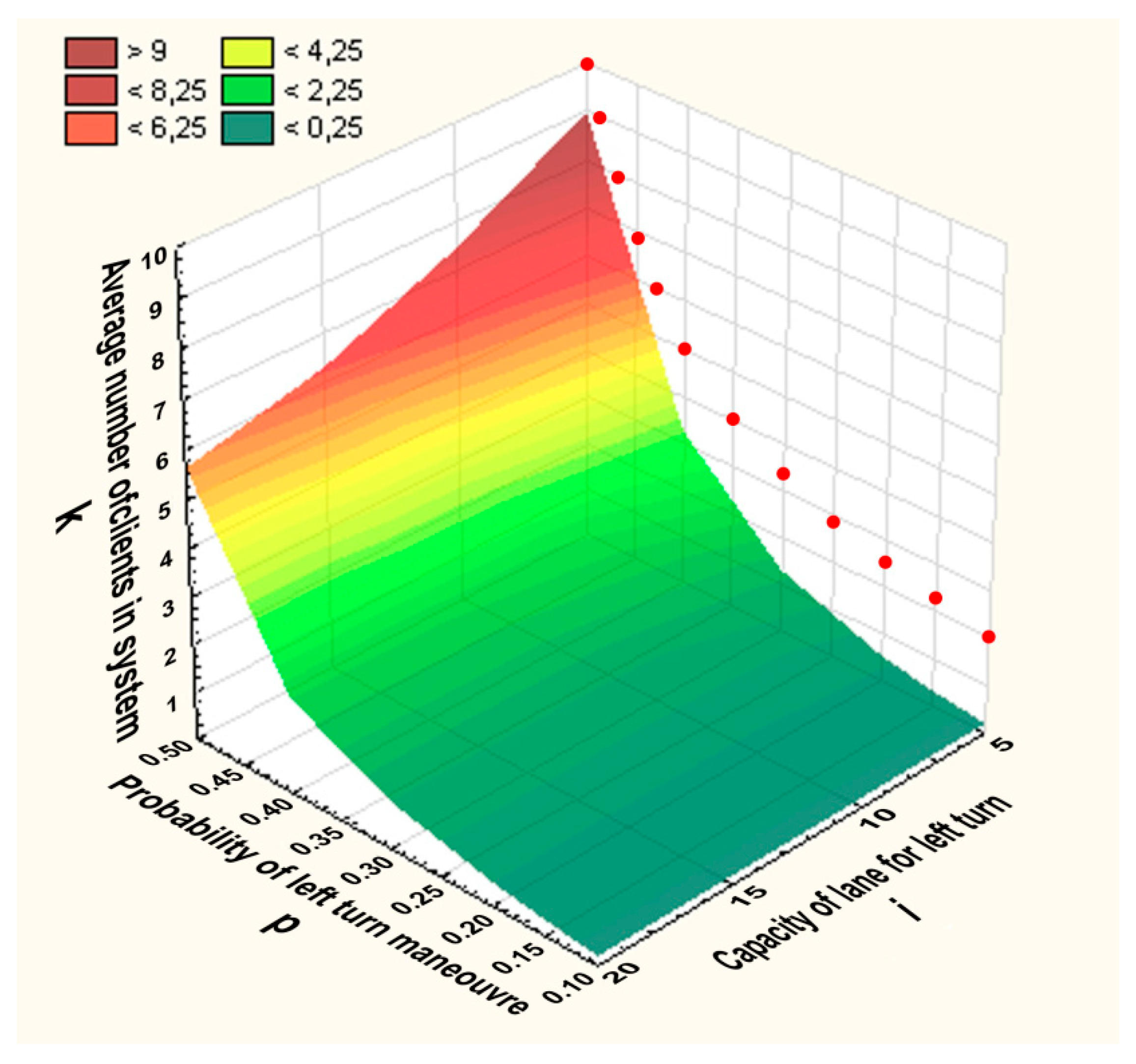
7. Results for Maximal Lane Capacity of Unsignalized Intersection

Figure 8 presents the average number of vehicles in the system for λ = 500 vehicle/h, μ = 300 vehicle/h (λ + μ = 800 vehicle/h, maximal lane capacity of unsignalized intersection established by Lakkundi [35], i∈[5, 20], and p∈[0.10, 0.50]. The maximal number of vehicles in the system is marked in the figure at i = 0 and calculated according to (25) for different probabilities “p” (emphasized by red dots). The average number of vehicles has been calculated according to expressions (47)–(49). From Figure 8, it can be seen that probability “p” (with which vehicles from the priority direction decide to make a left turn) has more effect than number of places in the short lane “i”.

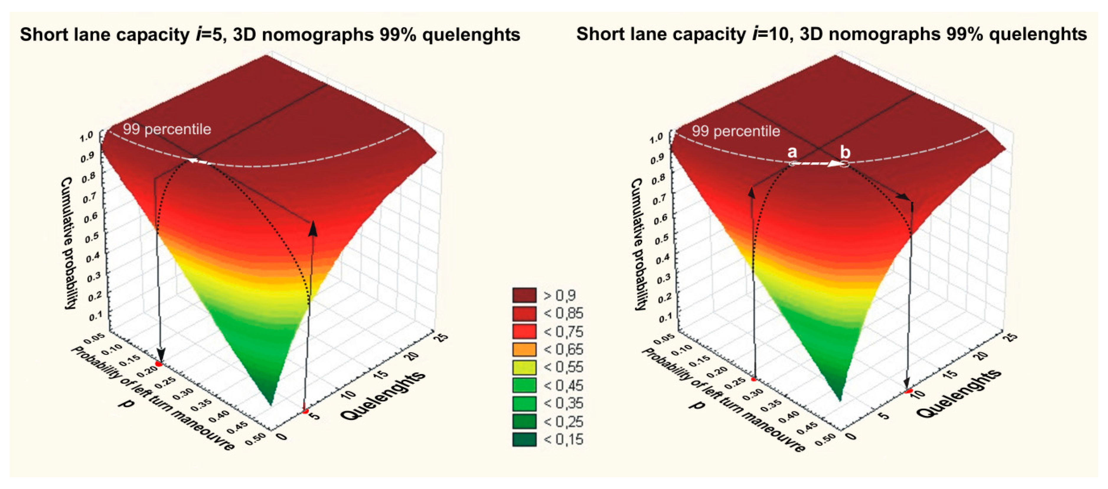
For the given parameters, namely, λ = 500 vehicle/h and μ = 300 vehicle/h, two nomographic distributions for the queue lengths can be expressed by using the cumulative probabilities - analogous to the usage of (P_0,0 + … + P_i,0 + P_i,1 + P_i,2 + …). A 3D function of the independent variable of the short lane “i” and probability of the left-turn maneuver “p” is presented in Figure 9.

In the first case, for i = 5, it can be noted that 99% of the vehicles will be satisfied up to p = 0.20. This implies that for a short lane with a capacity of five places for vehicles, 99% of the vehicles will not use the capacity of the shared lane for forming a queue if p = 0.20, without queue overflow/short lane saturation. This is apriori consideration of capacity.

Table 1. Cumulative probability calculation for 3D nomograph i = 5, short lane capacity i∈[1, 20], left turn probability p∈[0.05, 0.40].

i	p = 0.05	p = 0.10	p = 0.15	p = 0.20	p = 0.25	p = 0.30	p = 0.35	p = 0.40
1	0.917	0.833	0.749	0.663	0.574	0.482	0.388	0.295
2	0.993	0.972	0.936	0.884	0.814	0.724	0.615	0.491
3	0.999	0.995	0.983	0.958	0.913	0.844	0.747	0.622
4	1.000	0.999	0.995	0.982	0.955	0.905	0.824	0.709
5	1.000	1.000	0.998	0.990	0.972	0.935	0.869	0.767
6	1.000	1.000	0.998	0.993	0.979	0.950	0.895	0.806
7	1.000	1.000	0.999	0.995	0.985	0.961	0.916	0.838
8	1.000	1.000	0.999	0.997	0.989	0.970	0.933	0.865
9	1.000	1.000	0.999	0.998	0.992	0.977	0.946	0.888
10	1.000	1.000	1.000	0.998	0.994	0.982	0.957	0.906
11	1.000	1.000	1.000	0.999	0.995	0.986	0.966	0.922
12	1.000	1.000	1.000	0.999	0.997	0.990	0.973	0.935
13	1.000	1.000	1.000	0.999	0.997	0.992	0.978	0.946
14	1.000	1.000	1.000	1.000	0.998	0.994	0.982	0.955
15	1.000	1.000	1.000	1.000	0.999	0.995	0.986	0.962
16	1.000	1.000	1.000	1.000	0.999	0.996	0.989	0.969
17	1.000	1.000	1.000	1.000	0.999	0.997	0.991	0.974
18	1.000	1.000	1.000	1.000	0.999	0.998	0.993	0.978
19	1.000	1.000	1.000	1.000	1.000	0.998	0.994	0.982
20	1.000	1.000	1.000	1.000	1.000	0.999	0.995	0.985

presents the calculation of cumulative probability. It is obvious that for p > 0.2 at given flow shared lane saturation begins.

In the second nomograph in Figure 9, an a posteriori problem is considered. Assumed, or in concrete case, statistical determined distribution of left turn is p = 0.27. From p = 0.27 ordinate on the surface of nomograph we reach intersection with line for percentile 99 - point “a”. By following the 99 percentile line we reach point “b”. From it, using the surface of nomograph we descend using ordinate reaching Queue lengths value which asses the value of capacity of short lane i ≈ 10! From the Table 1 concrete value can be calculated by interpolation. It is obvious that for i = 10 and p = 0.25 cumulative probability is 0.994 > 0.99, but for i = 10 and p = 0.30 cumulative probability is 0.986 > 0.99.

The chosen examples have a simple message: to increase probability from p = 0.2 to p = 0.27 or for 35%, short lane capacity doubled respectively from i = 5 to i = 10! Further growth of probability “p” disproportionally increases needed capacity of short lane. For example, for p = 0.35, λ = 500 vehicle/h and μ = 300 vehicle/h, short lane will satisfy 99% of traffic flow if the designed short lane capacity i ≥ 17 (see values in Table 1, values on gray background are less than 99 percentile). For values of limiting p_max = 0.375 (50) queue overflow/short lane saturation is permanent and separate lane for left-turn maneuvering (Figure 1) needs to be designed.

$$p_{\mathit{max}}=\frac{\mu }{\lambda +\mu }=\frac{300}{800}=0.375$$

(50)

To calculate the average time that a vehicle spends in a two-phase queueing system by using the Little formula, it is necessary to note that the intensity “pλ“ changes to “λ“ at state X_i,1 (Figure 7). Thus, the average time that a vehicle spends in the system is defined in (51), and k_i(I) is calculated according to (47) from states X_i,0 to X_i−1,0 (see Figure 7). Intensity “pλ“ is the arrival rate for states X_i,0 and X_i,1. Consequently, Little’s formula has the form:

$$\overline{t}=\frac{k_{i(I)}+i{P}_{i,0}+(i+1)P_{i,1}}{p\lambda }+\frac{{\displaystyle \sum _{j=2}^{\infty }(j+i)P_{i,j}}}{\lambda }$$

(51)

The average time that a vehicle spends in the system is largely, but not entirely, proportional to the average number of vehicles in the system.

8. Discussion

Existing methods for the calculation of shared–short lanes capacity are based on simulation software such as Highway Capacity Manual (HCM), Sidra Intersection, VISIT, etc. These methods are predominantly designed for signalized intersections.

For unsignalized intersections there is a previous method based on solving approximately queuing system from Wu [36] which is also verified by simulation. Development of this method lead to the presented analytical solution of complex recursive operations noted by Wu [2], too.

Transportation planners and policy makers have at their disposal a new analytical method for calculation of shared/short lanes for left turn capacity. According to Koenigsberg [25] it should be more precise in calculation and more sensitive to parameter variations when making decisions on design and reconstruction of capacity of shared/short lanes for the left turn.

For this reason, we emphasize that the key role in capacity calculation for shared/short lanes has the intensity of left turn “μ”. In theory, if this intensity is large or μ >> pλ, needed capacity “i” of shared/short lanes for left turn converges to zero and all the needs are satisfied by the shared lane. However in the opposite case, capacity of shared/short lanes for left turn diverges for minimal values of “p” and “λ”.This poses a question of justifiability of short lane for left turn design. Capacity with intensity “μ” is conditioned by density of priority (opposite) flow which can be calculated on standard unsignalized intersections [34] and non-standard unsignalized intersections [37]. Ultimately, intensity of left turn “μ” is an indirect product of traffic safety!

9. Conclusions

The significance of signalized intersection has proven to be more important than unsignalized intersections. Signalized intersections service a higher part of the traffic flow. This is the reason why the participation of signalized intersections in traffic safety and service quality is greater. The prevalent direction of researchers is justifiably in the direction of signalized intersections. For these reasons there are significant difference in solutions for signalized and unsignalized intersection occurs. If the fact that there are significantly more unsignalized intersections than signalized ones is taken into consideration, created difference can be declared as theoreticaldeficit.

Optimal dimensioning of short-shared line for left turn from priority direction is the predominant problem of unsignalized intersections. The proposed model is solved only for homogenous car flows, but can easily be adapted for heterogeneous flows with cyclists and pedestrians. For the generalization and calculation of heterogeneous system it is not necessary to change the structure of thequeuing system. Analytic background for adaption is in the well-known characteristic of adding up Poisson flows of different intensities which is proven in Raikov’s theorem from 1937. Based on a stated theoretical base, left turns from non−priority directions of unsignalized intersections can be easily solved.

With the possibility of practical application in intersection planning, this paper has brought a new solution in queuing theory. So far, binomial distribution through its relation with Poisson distribution has been used in monophasic homogenous Markovian queuing systems. The presented solution brings a new vision for solving multiphase heterogeneous queuing systems in which a client selectively decides on the service. In a small corps of existing solutions, once again it has been confirmed that the queuing system can be solved if client selection has binomial distribution. Future research can integrate different approaches like multi-criteria decision making methods [38,39].