Exploiting Weak Field Gravity-Maxwell Symmetry in Superconductive Fluctuations Regime


1
Dipartimento di Scienza Applicata e Tecnologia, Politecnico di Torino, corso Duca degli Abruzzi 24, 10129 Torino, Italy
2
National Research Nuclear University MEPhI, Kashirskoe shosse 31, 115409 Moscow, Russia
3
Istituto Nazionale di Fisica Nucleare, Sezione di Torino, via Pietro Giuria 1, 10125 Torino, Italy
*
Authors to whom correspondence should be addressed.
Symmetry 2019, 11(11), 1341; https://0-doi-org.brum.beds.ac.uk/10.3390/sym11111341
Submission received: 25 September 2019
/
Revised: 18 October 2019
/
Accepted: 20 October 2019
/
Published: 1 November 2019
(This article belongs to the Special Issue Symmetry and Quantum Gravity)
Abstract
:We study the behaviour of a superconductor in a weak static gravitational field for temperatures slightly greater than its transition temperature (fluctuation regime). Making use of the time-dependent Ginzburg–Landau equations, we find a possible short time alteration of the static gravitational field in the vicinity of the superconductor, providing also a qualitative behaviour in the weak field condition. Finally, we compare the behaviour of various superconducting materials, investigating which parameters could enhance the gravitational field alteration.
1. Introduction
It is since 1966, with the paper of DeWitt [1], that there has been great interest in the interplay between the theory of gravitation and superconductivity [2]. In the following years were produced a lot of theoretical papers about this topic [3,4,5,6,7,8,9,10,11,12,13,14,15,16,17,18,19,20,21,22], until Podkletnov and Nieminem claimed to have observed a gravitational shielding in a disk of YBaCuO (YBCO) [23], an high- superconductor (HTCS). Of course, after the publication of this paper, other groups tried to repeat the experiment obtaining controversial results [24,25,26,27,28,29,30], so that the question is still open.
Many researchers tried to give a theoretical explanation [31,32,33,34,35,36,37,38,39,40,41,42,43,44,45,46,47,48,49,50,51,52] of the experimental results of Podkletnov and Nieminem in subsequent years, although, in our opinion, the clearest work was made by Modanese in 1996 [53,54], interpreting the experimental results in the frame of a quantum field formulation. However, the complexity of the formalism makes it difficult to extract quantitative predictions.
In a previous work [55], we determined the possible alteration of a static gravitational field in a superconductor making use of the time-dependent Ginzburg–Landau equations [56,57,58], providing also an analytic solution in the weak field condition [59,60]. Now, we develop quantitative calculations in a range of temperatures very close but higher than the critical temperature, in the regime of fluctuations [61].
2. Weak Field Approximation
Let us consider a nearly flat spacetime configuration (weak gravitational field) where the metric can be expanded as:
with small perturbation of the flat Minkowski metric; we work in the mostly plus convention, . The inverse metric in the linear approximation is given by
and the Christoffel symbols, to linear order in are written as
The Riemann tensor is defined as
while the Ricci tensor is given by the contraction . To linear order in , the latter reads [55]
with . The Einstein equations [62,63] are written as
and the l.h.s. in first-order approximation reads
If we now define the tensor
the Einstein equations can be rewritten in the compact form:
We can impose a gauge fixing using the harmonic coordinate condition [62]:
also called De Donder gauge. The requirement of a coordinate condition plays the role of a gauge fixing, uniquely determining the physical configuration and removing indeterminacy; in harmonic coordinates, the metric satisfies a manifestly Lorenz-covariant condition, so that the De Donder gauge becomes a natural choice. Moreover, if one considers the weak-field expansion of the Einstein-Hilbert action in De Donder gauge, the action itself (as well as the graviton propagator) takes a particularly simple form. If we now use Equations (1) and (3) in the last of previous (12), we find, in first-order approximation
that is, we have the relations
that, in turns, imply the Lorenz gauge condition:
The above result simplifies expression (10) for , which takes the form
2.1. Gravito-Maxwell Equations
First, we find
Then, one also has
using Equation (11) and having defined . If we take the curl of , we obtain
while, for the curl of ,
using again Equation (11) and having defined .
Following the above prescriptions, we obtained for the fields (17) the set of equations:
having restored physical units [55]. This equations are formally equivalent to Maxwell equations, with and gravitoelectric and gravitomagnetic field respectively, having defined the vacuum gravitational permittivity and the vacuum gravitational permeability as:
2.2. Generalized Maxwell Equations
Now we introduce the generalized electric/magnetic field, scalar and vector potentials, containing both electromagnetic and gravitational terms:
where m and e are the mass and electronic charge, respectively, the subscripts identifying the electromagnetic and gravitational contributions. The generalized Maxwell equations for the fields (25) then become [55,66]:
with
where and are the electric permittivity and magnetic permeability in the vacuum, and and are the electric charge density and electric current density respectively.
We have shown how to define a new set generalized Maxwell equations for generalized electric and magnetic fields, in the limit of weak gravitational fields. In the following sections we will use this results to study the behaviour of a superconductor in the fluctuation regime, i.e. very close to its critical temperature .
3. The Model
The behaviour of a superconductor in the vicinity of its critical temperature has been extensively studied. This particular region of temperature is characterized by thermodynamic fluctuations of the order parameter, giving rise to a gradual increase of the resistivity of the material from zero to its normal state value, for temperatures . This happens because, above the critical temperature , the order parameter fluctuations create superfluid regions in which electrons are accelerated. For temperatures larger than , the average size of these regions is much greater than the mean free path, though it decreases with the rise in temperature of the sample.
The described regime can be studied by using the time-dependent Ginzburg-Landau equations [56]. Of course, we have to be sufficiently far from the critical point for this description to be valid (essentially we are dealing with a mean field theory). Moreover, here we suppose we deal with sufficiently dirty materials, in order to observe the effects of the fluctuations over a sizable range of temperature, i.e. the electronic mean free path ℓ in the normal material has to be less than 10 Å.
The time-dependent Ginzburg-Landau equations can be written, for temperatures larger than , with just the linear term, in the gauge-invariant form [67,68]:
where is the order parameter, is the potential vector and is the electric potential. Moreover, once defined , we also have
where is the BCS coherence length. If we put
we obtain two equations for the functions and :
where
is the superfluid speed and where the associated current density is
Now, we consider a fluctuation of the wave vector for the function f. Let be the value of f for a fluctuation of the wave vector . The above equations can be recast in a more convenient form:
where the last expression (34.ii) is obtained by using Equation (32) and and taking the gradient of Equation (31.ii). By integrating (34.ii) from zero to t, we obtain
so that is given by
with as it was calculated in [69]. Then, the current can be written as
At this point we sum over . The simpler situation is a three-dimensional sample whose dimensions are greater than the correlation length , so that we obtain
The potential vector can be calculated from:
when the time variations of external fields are small. The generalized electric field of Equation (25), in the case under consideration, can be written as
where we have considered the static weak (Earth-surface) gravitational field contribution , and where is a geometrical factor that depends on the shape of the superconductor and on the space point where we calculate the gravitational fluctuations caused by the presence of the superconductor itself. Of course, when we are in the weak field regime and we can neglect the term proportional to in the exponential. In the latter case, for the realisation of an experiment, one needs a weak magnetic field (we are around ) in order to have the superconductor in the normal state, and turn off the magnetic field at the time .
4. Results
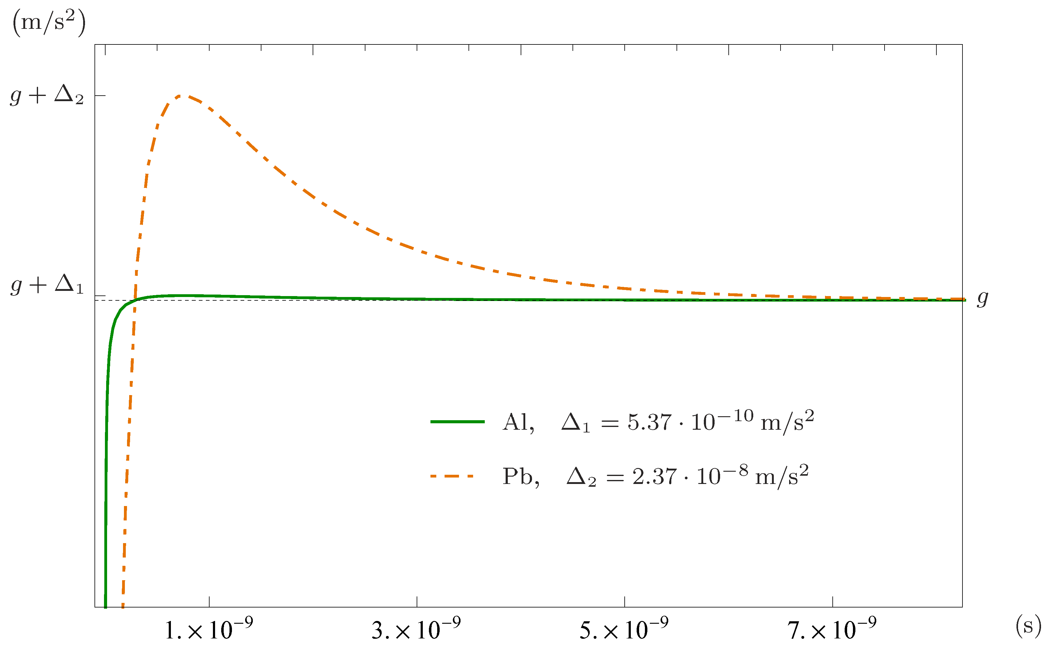
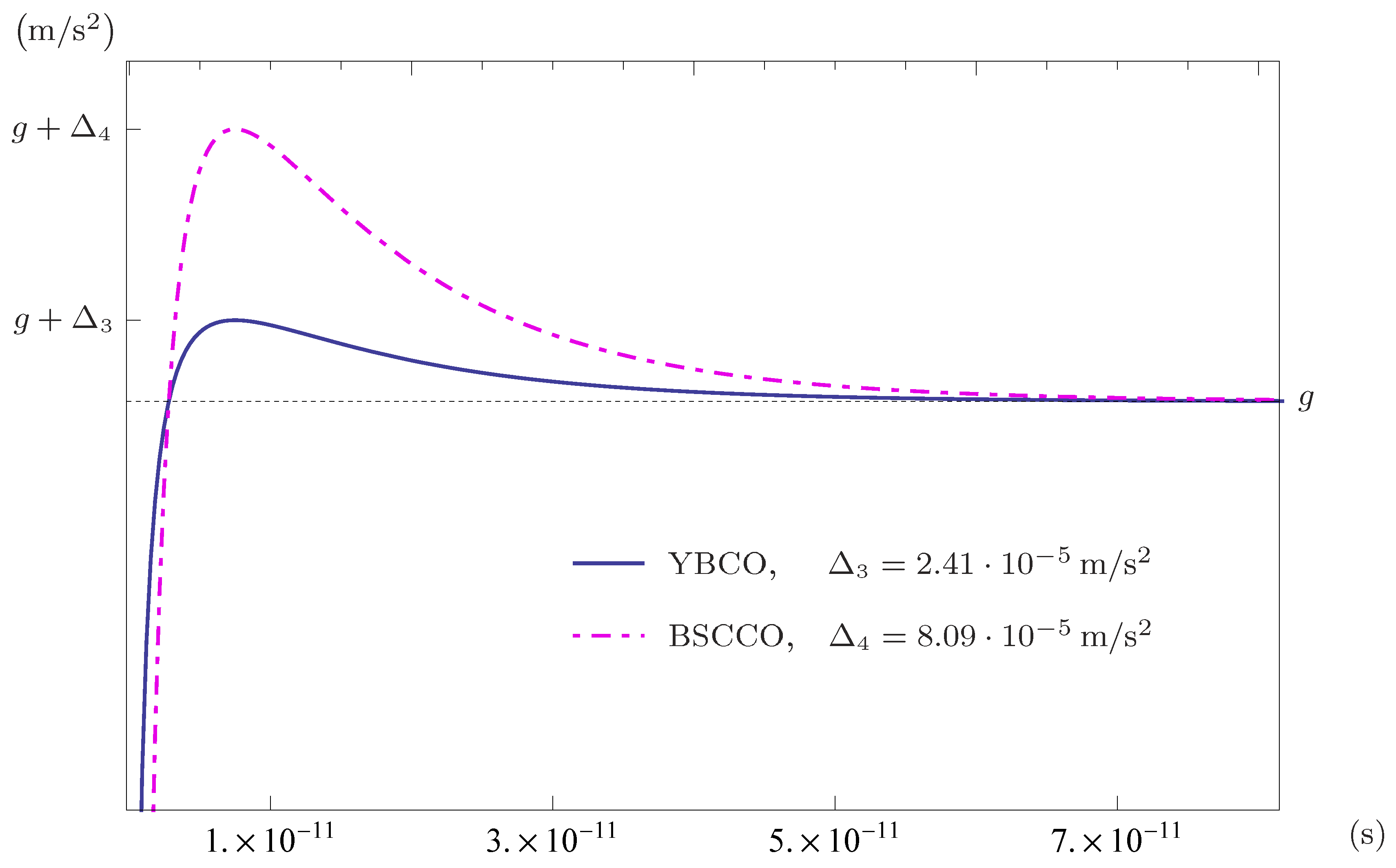
In Figure 1 and Figure 2 we show the variation of the gravitational field as a function of time, measured on the axis of a superconductive disk with bases parallel to the ground, at a fixed distance d from the surface, respectively for low- (Al and Pb) and high- superconductors (YBCO and BSCCO). The effect is calculated in the range of temperature where superconductive fluctuations are present. The system is initially at a temperature very close to , and is put it in the normal state by using a weak static magnetic field (near the upper critical field tends to zero). At the time , the magnetic field is removed so that the system goes in the superconductive state.
It is interesting to note that, in a very short initial time interval, the gravitational field is reduced w.r.t. its unperturbed value. After that, it increases up to a maximum value at the time and then decreases to the standard external value. In our previous paper, in the regime under , we found a weak shielding of the external gravitational field [55], with the corresponding solution for a simple case. The value is the maximum variation of the external gravitational field: in principle, field variation is measurable (especially in high- superconductors), while the problem lies in the very short time intervals in which the effect manifests itself.
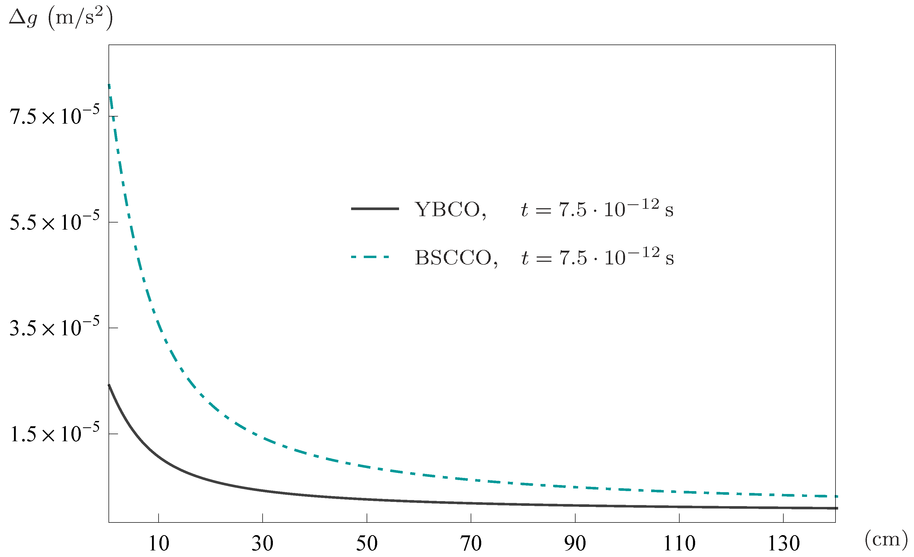
In Figure 3 it is shown the field variation effect as a function of distance from the disk surface, measured along the axis of the disk at the fixed time that maximizes the effect. In Table 1 we summarize the experimental data for the superconductive materials under consideration.
It is instructive to study the values of the parameters that maximize the effect in intensity and time interval. After simple but long calculations, it is possible to demonstrate that , so it is fundamental to be very close to the critical temperature in order to increase the time range in which the effect takes place. The maximum value of the correction for the external field is obtained for and is proportional to : this means that the effect is larger in high- superconductors, having the latter small coherence length. Clearly this behaviour makes the experimental detection difficult, since if we are close to we find an increase for the value of together with a decrease for the alteration of gravitational field, owing to the coherence length divergence at .
5. Conclusions
We have calculated the possible alteration of a static gravitational field in the vicinity of a superconductor in the regime of fluctuations. We have also shown that the effect should be weak (though perceptible), but it occurs in very short time intervals, making direct measurements difficult to obtain. Probably some ingredient for a complete depiction of the gravity-superfluid interaction has to be included, as long as it exists, for a more detailed characterization of the phenomenon.
Clearly, the goal is to obtain non-negligible experimental evidences (gravitational field perturbations) in workable time scales, trying to optimize contrasting effects by choosing appropriate temperature and sample coherence length. At present, the best option is to choose a HTCS (since very short coherence length increases the intensity of perturbation) and put the system at a temperature very close to (increase of time range where the effect occurs). It is also possible that the simultaneous presence of an electromagnetic field with particular characteristics, together with a suitable setting for the geometry of the experiment, could increase the magnitude of the effects under consideration.
Author Contributions
Both authors contributed to conceptualization, methodology and formal analysis.
Funding
This research received no external funding.
Acknowledgments
This work was supported by the MEPhI Academic Excellence Project (contract No. 02.a03.21.0005) for the contribution of G. A. Ummarino. We also thank Fondazione CRT ![Symmetry 11 01341 i001]() that partially supported this work for dott. A. Gallerati.
that partially supported this work for dott. A. Gallerati.
 that partially supported this work for dott. A. Gallerati.
Conflicts of Interest
The authors declare no conflict of interest.
References
- DeWitt, B.S. Superconductors and gravitational drag. Phys. Rev. Lett. 1966, 16, 1092–1093. [Google Scholar] [CrossRef]
- Kiefer, C.; Weber, C. On the interaction of mesoscopic quantum systems with gravity. Ann. Phys. 2005, 14, 253–278. [Google Scholar] [CrossRef] [Green Version]
- Papini, G. Detection of inertial effects with superconducting interferometers. Phys. Lett. A 1967, 24, 32–33. [Google Scholar] [CrossRef]
- Papini, G. Superconducting and normal metals as detectors of gravitational waves. Lett. Nuovo Cim. 1970, 4S1, 1027–1032. [Google Scholar] [CrossRef]
- Rothen, F. Application de la theorie relativiste des phenomenes irreversible a la phenomenologie de la supraconductivite. Helv. Phys. Acta 1968, 41, 591. [Google Scholar]
- Rystephanick, R. On the london moment in rotating superconducting cylinders. Can. J. Phys. 1973, 51, 789–794. [Google Scholar] [CrossRef]
- Hirakawa, H. Superconductors in gravitational field. Phys. Lett. A 1975, 53, 395–396. [Google Scholar] [CrossRef]
- Minasyan, I. Londons equations in riemannian space. Doklady Akademii Nauk SSSR 1976, 228, 576–578. [Google Scholar]
- Anandan, J. Gravitational and rotational effects in quantum interference. Phys. Rev. D 1977, 15, 1448. [Google Scholar] [CrossRef]
- Anandan, J. Interference, gravity and gauge fields. IL Nuovo Cimento A (1965–1970) 1979, 53, 221–250. [Google Scholar] [CrossRef]
- Anandan, J. Relativistic thermoelectromagnetic gravitational effects in normal conductors and superconductors. Phys. Lett. A 1984, 105, 280–284. [Google Scholar] [CrossRef]
- Anandan, J. Relativistic gravitation and superconductors. Class. Quantum Grav. 1994, 11, A23. [Google Scholar] [CrossRef]
- Ross, D. The london equations for superconductors in a gravitational field. J. Phys. A Math. Gen. 1983, 16, 1331. [Google Scholar] [CrossRef]
- Felch, S.B.; Tate, J.; Cabrera, B.; Anderson, J.T. Precise determination of h/me using a rotating, superconducting ring. Phys. Rev. B 1985, 31, 7006–7011. [Google Scholar] [CrossRef] [PubMed]
- Dinariev, O.Y.; Mosolov, A. A relativistic effect in the theory of superconductivity. Soviet Phys. Doklady 1987, 32, 1987. [Google Scholar]
- Peng, H.; Torr, D.; Hu, E.; Peng, B. Electrodynamics of moving superconductors and superconductors under the influence of external forces. Phys. Rev. B 1991, 43, 2700. [Google Scholar] [CrossRef] [PubMed]
- Peng, H. A new approach to studying local gravitomagnetic effects on a superconductor. Gen. Relat. Grav. 1990, 22, 609–617. [Google Scholar] [CrossRef]
- Peng, H.; Lind, G.; Chin, Y. Interaction between gravity and moving superconductors. Gen. Relat. Grav. 1991, 23, 1231–1250. [Google Scholar] [CrossRef]
- Li, N.; Torr, D. Effects of a gravitomagnetic field on pure superconductors. Phys. Rev. D 1991, 43, 457. [Google Scholar] [CrossRef]
- Li, N.; Torr, D.G. Gravitational effects on the magnetic attenuation of superconductors. Phys. Rev. B 1992, 46, 5489. [Google Scholar] [CrossRef]
- Torr, D.G.; Li, N. Gravitoelectric-electric coupling via superconductivity. Found. Phys. Lett. 1993, 6, 371–383. [Google Scholar] [CrossRef]
- de Andrade, L.G. Torsion, superconductivity, and massive electrodynamics. Int. J. Theor. Phys. 1992, 31, 1221–1227. [Google Scholar] [CrossRef]
- Podkletnov, E.; Nieminen, R. A possibility of gravitational force shielding by bulk YBa2Cu3O7-X superconductor. Phys. C Supercond. 1992, 203, 441–444. [Google Scholar] [CrossRef]
- Li, N.; Noever, D.; Robertson, T.; Koczor, R.; Brantley, W. Static test for a gravitational force coupled to type II YBCO superconductors. Phys. C Supercond. 1997, 281, 260–267. [Google Scholar] [CrossRef]
- de Podesta, M.; Bull, M. Alternative explanation of “gravitational screening” experiments. Phys. C Supercond. 1995, 253, 199–200. [Google Scholar] [CrossRef]
- Unnikrishnan, C. Does a superconductor shield gravity? Phys. C Supercond. 1996, 266, 133–137. [Google Scholar] [CrossRef]
- Tajmar, M.; Plesescu, F.; Seifert, B. Measuring the dependence of weight on temperature in the low-temperature regime using a magnetic suspension balance. Meas. Sci. Technol. 2009, 21, 015111. [Google Scholar] [CrossRef]
- Tajmar, M. Evaluation of enhanced frame-dragging in the vicinity of a rotating niobium superconductor, liquid helium and a helium superfluid. Phys. C Supercond. 2011, 24, 125011. [Google Scholar] [CrossRef]
- Podkletnov, E.; Modanese, G. Investigation of high voltage discharges in low pressure gases through large ceramic superconducting electrodes. J. Low Temp. Phys. 2003, 132, 239–259. [Google Scholar] [CrossRef]
- Poher, C.; Modanese, G. Enhanced induction into distant coils by ybco and silicon-graphite electrodes under large current pulses. Phys. Essays 2017, 30, 435–441. [Google Scholar] [CrossRef]
- Ciubotariu, C.; Agop, M. Absence of a gravitational analog to the meissner effect. Gene. Relat. Grav. 1996, 28, 405–412. [Google Scholar] [CrossRef]
- Agop, M.; Buzea, C.G.; Griga, V.; Ciubotariu, C.; Buzea, C.; Stan, C.; Jatomir, D. Gravitational paramagnetism, diamagnetism and gravitational superconductivity. Aust. J. Phys. 1996, 49, 1063–1074. [Google Scholar] [CrossRef]
- Agop, M.; Ioannou, P.; Diaconu, F. Some implications of gravitational superconductivity. Prog. Theor. Phys. 2000, 104, 733–742. [Google Scholar] [CrossRef]
- Agop, M.; Buzea, C.G.; Nica, P. Local gravitoelectromagnetic effects on a superconductor. Phys. C Supercond. 2000, 339, 120–128. [Google Scholar] [CrossRef]
- Ivanov, B. Gravitational effects in a spherical solenoid. Mod. Phys. Lett. A 1997, 12, 285–294. [Google Scholar] [CrossRef]
- Ahmedov, B. General relativistic thermoelectric effects in superconductors. Gen. Relat. Grav. 1999, 31, 357–369. [Google Scholar] [CrossRef]
- Ahmedov, B.; Kagramanova, V. Electromagnetic effects in superconductors in stationary gravitational field. Int. J. Mod. Phys. D 2005, 14, 837–847. [Google Scholar] [CrossRef]
- Tajmar, M.; de Matos, C.J. Gravitomagnetic field of a rotating superconductor and of a rotating superfluid. Physica 2003, C385, 551–554. [Google Scholar] [CrossRef]
- de Matos, C.J.; Tajmar, M. Gravitomagnetic London moment and the graviton mass inside a superconductor. Physica 2003, C432, 167. [Google Scholar] [CrossRef]
- Tajmar, M.; de Matos, C.J. Extended analysis of gravitomagnetic fields in rotating superconductors and superfluids. Physica 2005, C420, 56. [Google Scholar] [CrossRef]
- Tajmar, M. Electrodynamics in superconductors explained by proca equations. Phys. Lett. A 2008, 372, 3289–3291. [Google Scholar] [CrossRef]
- Ning, W. Gravitational shielding effect in gauge theory of gravity. Commun. Theor. Phys. 2004, 41, 567. [Google Scholar] [CrossRef]
- Chiao, R.Y. The interface between quantum mechanics and general relativity. J. Mod. Opt. 2006, 53, 16–17. [Google Scholar] [CrossRef]
- de Matos, C.J. Gravitoelectromagnetism and dark energy in superconductors. Int. J. Mod. Phys. D 2007, 16, 2599–2606. [Google Scholar] [CrossRef]
- de Matos, C.J. Electromagnetic dark energy and gravitoelectrodynamics of superconductors. Phys. C Supercond. 2008, 468, 210–213. [Google Scholar] [CrossRef] [Green Version]
- de Matos, C.J. Gravitational force between two electrons in superconductors. Phys. C Supercond. 2008, 468, 229–232. [Google Scholar] [CrossRef] [Green Version]
- de Matos, C.J. Physical vacuum in superconductors. J. Supercond. Novel Magn. 2010, 23, 1443–1453. [Google Scholar] [CrossRef]
- de Matos, C.J. Modified entropic gravitation in superconductors. Phys. C Supercond. 2012, 472, 5–9. [Google Scholar] [CrossRef] [Green Version]
- Inan, N.; Thompson, J.; Chiao, R. Interaction of gravitational waves with superconductors. Fortschritte der Physik 2017, 65, 1600066. [Google Scholar] [CrossRef]
- Inan, N. A new approach to detecting gravitational waves via the coupling of gravity to the zero-point energy of the phonon modes of a superconductor. Int. J. Mod. Phys. D 2017, 26, 1743031. [Google Scholar] [CrossRef]
- Atanasov, V. The geometric field (gravity) as an electro-chemical potential in a ginzburg-landau theory of superconductivity. Phys. B Cond. Matter 2017, 517, 53–58. [Google Scholar] [CrossRef]
- Sbitnev, V.I. Quaternion algebra on 4d superfluid quantum space-time: Gravitomagnetism. Found. Phys. 2019, 49, 107–143. [Google Scholar] [CrossRef]
- Modanese, G. Theoretical analysis of a reported weak-gravitational-shielding effect. EPL (Europhys. Lett.) 1996, 35, 413. [Google Scholar] [CrossRef]
- Modanese, G. Role of a “local” cosmological constant in euclidean quantum gravity. Phys. Rev. D 1996, 54, 5002. [Google Scholar] [CrossRef]
- Ummarino, G.A.; Gallerati, A. Superconductor in a weak static gravitational field. Eur. Phys. J. 2017, C77, 549. [Google Scholar] [CrossRef]
- Cyrot, M. Ginzburg-landau theory for superconductors. Rep. Prog. Phys. 1973, 36, 103–158. [Google Scholar] [CrossRef]
- Zagrodziński, J.; Nikiciuk, T.; Abal’osheva, I.; Lewandowski, S. Time-dependent ginzburg–landau approach and its application to superconductivity. Supercond. Sci. Technol. 2003, 16, 936. [Google Scholar] [CrossRef]
- Alstrøm, T.S.; Sørensen, M.P.; Pedersen, N.F.; Madsen, S. Magnetic flux lines in complex geometry type-ii superconductors studied by the time dependent ginzburg-landau equation. Acta Appl. Math. 2011, 115, 63–74. [Google Scholar] [CrossRef]
- Mashhoon, B.; Paik, H.J.; Will, C.M. Detection of the gravitomagnetic field using an orbiting superconducting gravity gradiometer. theoretical principles. Phys. Rev. D 1989, 39, 2825–2838. [Google Scholar] [CrossRef]
- Ruggiero, M.L.; Tartaglia, A. Gravitomagnetic effects. IL Nuovo Cimento B 2002, 117, 743–768. [Google Scholar]
- Larkin, A.; Varlamov, A. Fluctuation Phenomena in Superconductors. In Handbook on Superconductivity: Conventional and Unconventional Superconductors; Springer: Berlin, Germany, 2002; p. 1. [Google Scholar]
- Wald, R.M. General Relativity; University of Chicago Press: Chicago, IL, USA, 1984; p. 491. [Google Scholar]
- Misner, C.W.; Thorne, K.S.; Wheeler, J.A. Gravitation; Macmillan: London, UK, 1973. [Google Scholar]
- Braginsky, V.B.; Caves, C.M.; Thorne, K.S. Laboratory experiments to test relativistic gravity. Phys. Rev. D 1977, 15, 2047. [Google Scholar] [CrossRef]
- Huei, P. On calculation of magnetic-type gravitation and experiments. Gen. Relat. Grav. 1983, 15, 725–735. [Google Scholar] [CrossRef]
- Behera, H. Comments on gravitoelectromagnetism of Ummarino and Gallerati in “Superconductor in a weak static gravitational field” vs. other versions. Eur. Phys. J. 2017, C77. [Google Scholar] [CrossRef]
- Hurault, J. Nonlinear effects on the conductivity of a superconductor above its transition temperature. Phys. Rev. 1969, 179, 494. [Google Scholar] [CrossRef]
- Schmid, A. Diamagnetic susceptibility at the transition to the superconducting state. Phys. Rev. 1969, 180, 527. [Google Scholar] [CrossRef]
- de Gennes, P.-G. Superconductivity of Metals and Alloys; CRC Press: Boca Raton, FL, USA, 2018. [Google Scholar]
Figure 1.
The variation of gravitational field as a function of time in the vicinity of a superconductive sample of Al (green solid line) and one of Pb (orange dot-dashed line). The field is measured along the axis of the disk, with bases parallel to the ground, at a fixed distance above the disk surface. The radius of the disk is and the thickness is .

Figure 2.
The variation of gravitational field as a function of time in the vicinity of a superconductive disk of YBCO (blue solid line) and BSCCO (purple dot-dashed line). The field is measured along the axis of the disk, with bases parallel to the ground, at a fixed distance above the disk surface. The radius of the disk is and the thickness is .

Figure 3.
The variation of gravitational field as a function of distance in the vicinity of a superconductive sample of YBCO (grey solid line) and one of BSCCO (light blue dot-dashed line). The field is measured along the axis of the disk, with bases parallel to the ground, at the fixed time that maximizes the variation. The radius of the disk is and the thickness is .


Table 1.
Input and output parameters for the four different superconductors.
| Al | 15500 | 531313 | ||||
| Pb | 870 | 73924 | ||||
| YBCO | 30 | 895 | ||||
| BSCCO | 10 | 333 |
© 2019 by the authors. Licensee MDPI, Basel, Switzerland. This article is an open access article distributed under the terms and conditions of the Creative Commons Attribution (CC BY) license (http://creativecommons.org/licenses/by/4.0/).
Share and Cite
MDPI and ACS Style
Ummarino, G.A.; Gallerati, A. Exploiting Weak Field Gravity-Maxwell Symmetry in Superconductive Fluctuations Regime. Symmetry 2019, 11, 1341. https://0-doi-org.brum.beds.ac.uk/10.3390/sym11111341
AMA Style
Ummarino GA, Gallerati A. Exploiting Weak Field Gravity-Maxwell Symmetry in Superconductive Fluctuations Regime. Symmetry. 2019; 11(11):1341. https://0-doi-org.brum.beds.ac.uk/10.3390/sym11111341
Chicago/Turabian StyleUmmarino, Giovanni Alberto, and Antonio Gallerati. 2019. "Exploiting Weak Field Gravity-Maxwell Symmetry in Superconductive Fluctuations Regime" Symmetry 11, no. 11: 1341. https://0-doi-org.brum.beds.ac.uk/10.3390/sym11111341
Note that from the first issue of 2016, this journal uses article numbers instead of page numbers. See further details here.