A Haptic Model of Entanglement, Gauge Symmetries and Minimal Interaction Based on Knot Theory


Institut für Didaktik der Physik, Universität Münster, 48149 Münster, Germany
*
Author to whom correspondence should be addressed.
†
Current address: Wilhelm-Klemm-Str. 10, 48149 Münster, Germany.
Symmetry 2019, 11(11), 1399; https://0-doi-org.brum.beds.ac.uk/10.3390/sym11111399
Submission received: 23 October 2019
/
Revised: 6 November 2019
/
Accepted: 8 November 2019
/
Published: 12 November 2019
Abstract
:The Heegaard splitting of is a particularly useful representation for quantum phases of spin j-representation arising in the mapping , which can be related to torus knots in Hilbert space. We show that transitions to homotopically equivalent knots can be associated with gauge invariance, and that the same mechanism is at the heart of quantum entanglement. In other words, (minimal) interaction causes entanglement. Particle creation is related to cuts in the knot structure. We show that inner twists can be associated with operations with the quaternions , which are crucial to understand the Hopf mapping . We discuss the relationship between observables on the Bloch sphere , and knots with inner twists in Hilbert space. As applications, we discuss selection rules in atomic physics, and the status of virtual particles arising in Feynman diagrams. Using a simple paper strip model revealing the knot structure of quantum phases in Hilbert space including inner twists, a model of entanglement and gauge symmetries is proposed, which may also be valid for physics education.
1. Introduction
The importance of topology for various applications in physics is constantly increasing, in particular, in quantum information theory [1,2]. Recently, a haptic ‘paper strip’ model for quantum phases of spin j-states was introduced, which generalizes the Dirac belt describing a spin particle, to general spin j in Hilbert space [3,4].
In this paper, we show that quantum entanglement and gauge symmetries can also be modeled using that paper strip representation of the emerging knots. In all cases, unitary time development is at the heart of the physical problems, thus, the geometry of is the common feature that must be understood. In Section 2 and Section 3, we study the situation for in detail, based on the Heegaard splitting and the paper strip model of quantum phases for spin j-representations [3], and the Hopf mapping to the Bloch sphere. In particular, we argue that albeit the usual Bloch sphere representation is sufficient for the description of observables, crucial features in Hilbert space which will be relevant for our haptic model of entanglement and gauge symmetry are invisible, since knots can only arise in Hilbert space. In Section 4, we apply the paper strip model to the -Chern–Simons gauge field and discuss the importance of inner twists in addition to the knot structure.
In Section 5, the simplest example for quantum entanglement is described, arising due to the -interaction between two qubits. We propose a haptic model of Bell states based on transitions to homotopically equivalent knots in Hilbert space. In Section 6, gauge symmetries are introduced in close analogy to entanglement arising due to (minimal) interaction. As applications, we consider selection rules in atomic physics, and the role of Feynman diagrams in QED. In both cases, transitions to homotopically equivalent knots describing the quantum phase are the key ingredient of our model, revealing the close relation between minimal interaction and entanglement.
The main purpose of the present paper is the introduction of haptic models giving some topological insights into some key ideas of modern physics. If we compare mathematics to a musical score, then in case of music the direct and more intuitive representation of music as soundwave is obvious. In some sense, we try to reveal this direct and more intuitive representation that is hidden within the mathematical formalism of modern quantum physics using haptic models and visualizations.
2. The Hopf Mapping for a Single Qubit
We introduce the standard basis for an arbitrary qubit. The general (pure) orthonormal superposition states of a qubit are given by and , with complex amplitudes fulfilling . Geometrically, all these spin states form the hypersphere in four dimensions. In many applications, the geometry of is not considered in detail, as observables such as e.g., are obtained after Hopf mapping , where denote the Pauli matrices. As shown in Figure 1, the difference between the probabilities for the eigenvalues define the coordinates of the vector on the Bloch sphere, which just defines the Hopf mapping in case of spin [5,6]. Please note that the state orthogonal to is mapped to the vector on the Bloch sphere.
In this paper, we want to show that a more detailed understanding of the geometry of the qubit (and its generalization to higher spin states) in is important not only in order to reveal the knot structure of bosonic and fermionic quantum states, but also to find some appropriate models for gauge interaction and entanglement.
First, we introduce some coordinates on . Similar to [4], we introduce the homogeneous coordinates , and define the mapping as . The single complex coordinate z on is equivalent to the Bloch sphere via stereographic projection, . All observables can be described on the Bloch sphere (or ), which is -periodic. For this reason, we denote as ‘-realm’. The points are different on , which means that in , periodicity is doubled to . Indeed, introducing the quaterions as
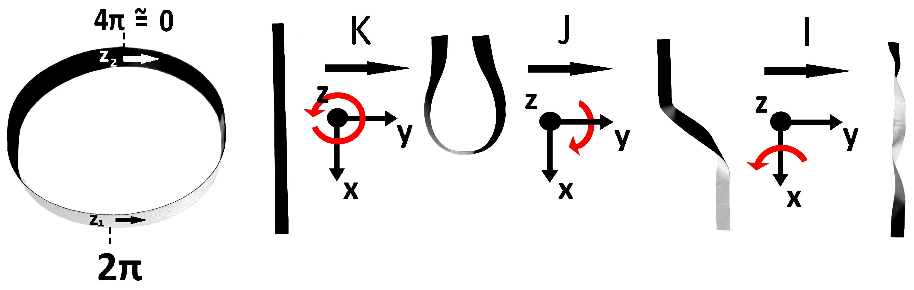
we may view the sign change as a rotation around in , since . Only after a -rotation, the original point is reached, . For this reason, we call the ‘-realm’. The operations with quaternions induce on the (generalized) Dirac belt as shown in Figure 2.
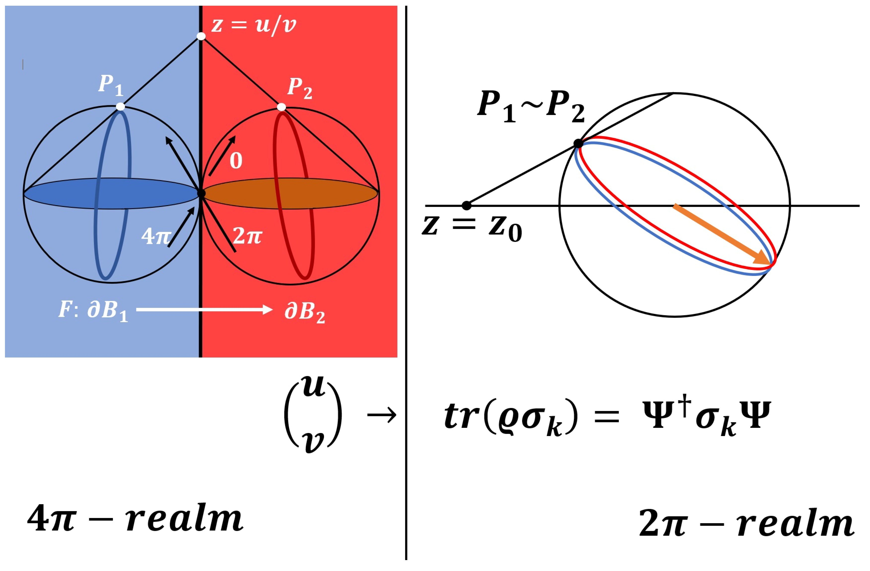
We want to introduce the so-called Heegaard splitting of [7], which is convenient to describe the relation between the -realm and the -realm. The geometry of can be seen as two unit balls and in three dimensions, where the two-dimensional boundaries and are identified via a homeomorphism (The Heegaard splitting of can also be done using the boundary of torus and identified via a homeomorphism). Using this decomposition, the Hopf mapping can be understood as follows: In , (torus) knots emerge for the spin j representation with [3]. The knot structure in the full Hilbert space—the -realm - is projected to the boundary, where observables are defined—the -realm. This mapping is 2:1, since the knots in the two unit balls and are projected to the boundaries and , which are then identified by to become . After stereographic projection, the structure in the three-dimensional bulk is mapped to a structure on the boundary, which is nothing but the Bloch sphere as shown in Figure 3 and Figure 4 for the case . Here, the so-called Dirac belt describing the quantum phase of spin states emerges in . The Heegaard splitting helps to visualize the homotopy mappings and . Indeed, two traversals of a great circle on are necessary to complete the homotopy in , see Figure 3. Using the paper strip model, the relation between inner twists and the Möbius strip can easily be derived by considering the double traversal . Due to the four inner twists, the Dirac belt it is equivalent to a Möbius strip, which is mapped after identification of the boundaries and to the stellar representation . The node corresponds to the point of the Bloch sphere, since the amplitude of the state vanishes at .
We want to model the relation between knots and nodes using the paper strip model using the explicit coordinates
We choose the qubits in the standard basis, described by the vectors and and corresponding nodes at the antipodes, as shown in Figure 5 (in the stellar representation, these nodes would be mapped to and ). The probability to detect the eigenvalue at position is given by and . We wish to model the homotopy on the equatorial line with . Here, the corresponding amplitudes (for ) are and . In the paper strip model, these amplitudes can be modeled as Möbius strips with one right-moving (R) and with one left-moving (L) twist, respectively. The Heegard splitting also helps to visualize the homotopy mappings and . Indeed, a double winding on is necessary to complete the homotopy in , see Figure 3.
For the superposition state , the corresponding amplitude at is given by which indeed has a node at , i.e., at .
However, this is not the most general situation in . We have chosen a particularly suitable homotopy, where the Dirac belt has already been glued together when we traverse twice the equatorial line in . In general, the homotopy can be anywhere in the unit balls and , and describe a Dirac belt with four inner twists, as depicted in Figure 4. The superposition translates into a knot theoretic relation, which—in a somewhat sloppy notation—is shown in Figure 4. Here, it is sufficient to note that the nodes on the Bloch sphere indeed translate to knots in . The exact relations valid for Homfley-polynomials are discussed in [8]. Please note that the Dirac belt would be equivalent to the trivial knot, if inner twists were ignored.
3. Knots and Inner Twists for Spin j States
Here, defines a -to-one mapping [9].
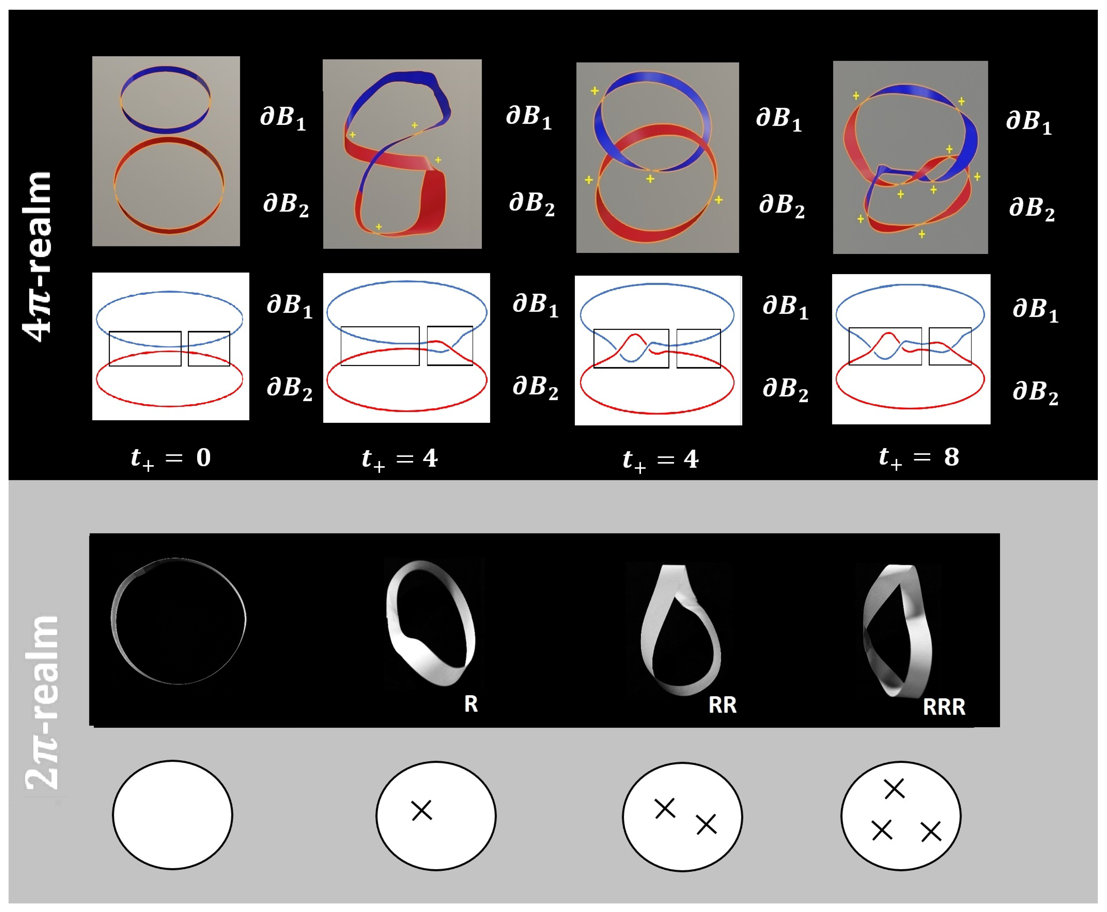
Using the paper strip model, it is possible to map the quantum phase related to the homotopy for a spin j representation from the -realm to the -realm. As shown in Figure 6, we may choose the knot structure to be close to the boundaries and . The are mapped to as shown in Figure 6 due to the Hopf mapping. We can distinguish five different representations:
- The knot in the -realm including inner twists ( for bosons, for fermions), modeled with the paper strip in the -realm.
- The corresponding Jones polynomial , describing the knot structure of the spin j state on a homotopic loop in the -realm ignoring inner twists.
- The quantum phase of the observable in the -realm with twists, obtained by ‘gluing together’ the two parts of the knot on the surface upon identification of the two pieces and .
- The corresponding stellar representation on given by with nodes and .
- Stereographic projection of the stellar representation on the Bloch sphere . For bosons with the result is equivalent to spherical harmonics .
4. A Haptic Model of Topological Gauge Fields
The main purpose of our paper is a topological understanding of gauge fields and entanglement. We the operations of quaternions on the state to motions in (and the corresponding -representation of )
For quaternions, the well-known identities
hold true and can be reproduced using the paper strip model shown in Figure 2 in the -realm [8]. Note that the operator corresponds to a rotation around and induces two inner twists .
As an application, we consider the well-known Chern–Simons action. We will not contribute anything new to the mathematical formalism; however, we want to model the interplay between the emerging knot structure in the -realm , and observables in the -realm in the paper strip model. These insights will be helpful for the main purpose of our paper, i.e., a haptic model of gauge symmetries and entanglement. We use the notations introduced in [10].
In imaginary time formalism, we define the 1-form with (the gauge field), and the two-form (the field strength). Then, the well-known relation
holds. The Chern–Simons action is then defined by
Interestingly, the relation between bulk (4D manifold M) and boundary (3D-manifold ) emerges again. Note, however, that the boundary is three-dimensional, allowing for a knot structure. From the gauge transformation
only the term makes a relevant contribution to the boundary integral , leading to
Here, the so-called winding number is given by [10]
where g is a general SU(2) gauge field with , and is the Haar measure of For the abelian case with and , this integral corresponds to . The Chern–Simons action and its knot theoretic implications have been extensively studied [11]. For our purpose, we want to focus on the importance of the interplay between knots including their inner twists, and the mapping to observables onto the (generalized) Bloch sphere. For this purpose, we want to show that the number of inner twists of configurations contained in g is related to the winding number (9) as .
For the standard mapping, choose with
We obtain for the standard mapping
and cyclic, i.e., for the standard mapping, (9) boils down to
The integral just gives the volume of . We wrote the explicit contributions to compare with Figure 2 to find the relation of this integral to our haptic model. Indeed, the number of inner twists of each configuration is .
As shown in [10], if the winding number of the gauge configuration and are given by and , then the winding number of is given by . Because the Chern–Simons action (9) is a homotopy invariant, it suffices to consider the following class of mappings
Since , due to the additivity of the winding number, it follows that for .
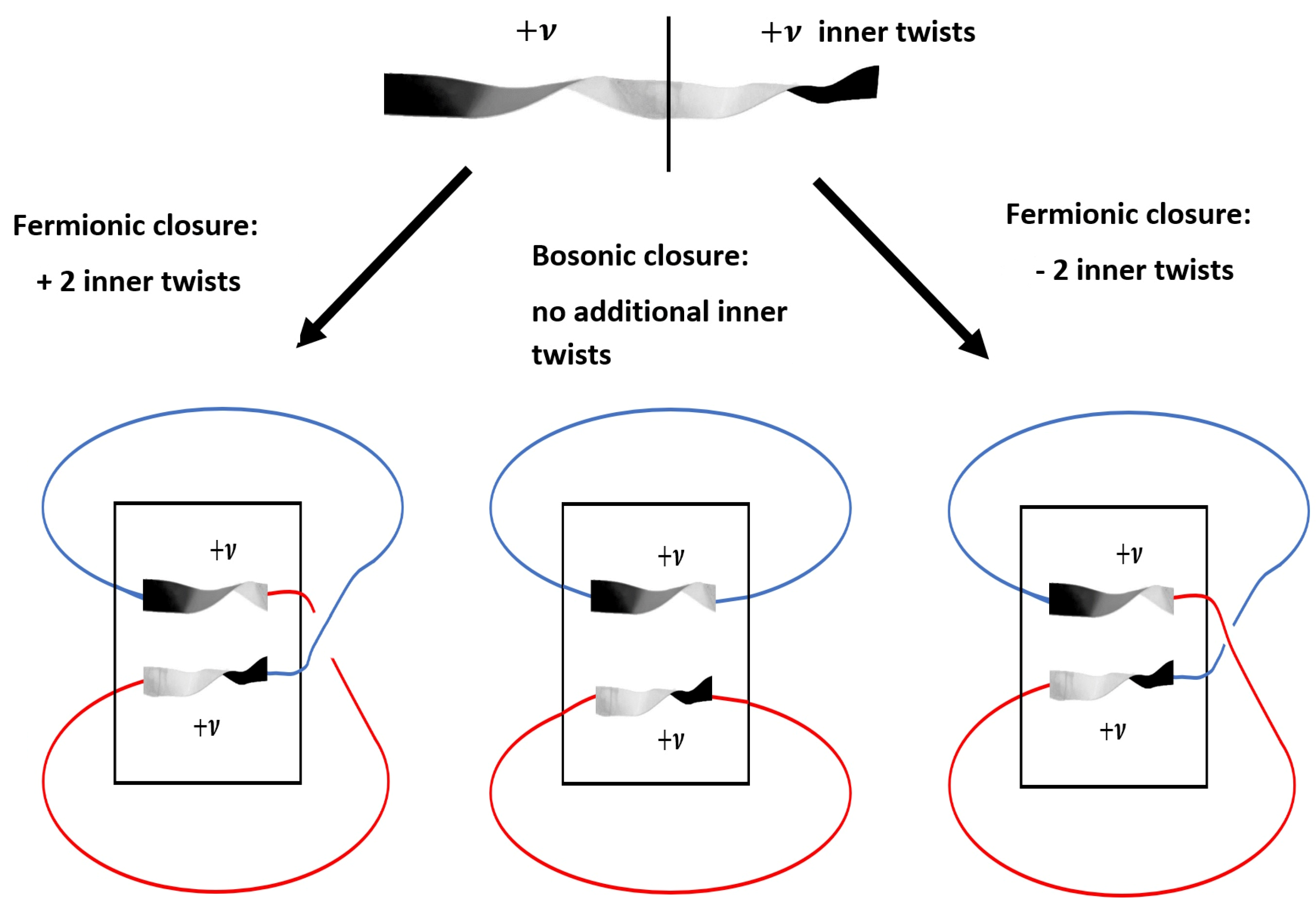
Next, suppose the Chern–Simons gauge field interacts with fermions. If we define , we find . On the level of the elements of the group, compared to (3), we conclude that the class with winding number contains knot structures up to spin . For observables, the number of inner twists is crucial. As shown in [4], the inner twists must be (additional to the knot structures as defined by Jones polynomial) equal to for fermions, and for bosons. Indeed, the mapping allows for inner twists. As shown in Figure 7, for a fermionic closure of the quantum phase, the number of inner twists is changed by . For bosons, the number remains the same. Indeed, for bosons, we obtain (corresponding to inner twists, related to nodes in the stellar representation and l nodal lines e.g., for spherical harmonics). For fermions, we obtain inner twists, corresponding to spin states with the odd number of nodes in the stellar representation.
Using the paper strip model of gauge interaction shown in Figure 12, sum rules can be derived for the interaction of gauge fields with quarks [10], leading to a topological interpretation of Ward-Takahashi identities. As this application of the paper strip model is not the main purpose of the present paper, details will be shown elsewhere.
It is instructive to relate the topological meaning of the Chern–Simons action with the Heegaard splitting. As shown in [8], the following relation holds
with the vacuum given by , compare Figure 3. Here, is a diffeomorphism connecting the two boundaries of the unit balls and with each other as
Indeed, this diffeomorphism just defines the knot structure contained in and can be described using the paper strip model.
5. A Haptic Model of Quantum Entanglement
To model entanglement using the paper strip model, we start with the simplest possible case, i.e., the interaction of two qubits. The most general pure two-qubit state is obtained as the orbit of the state , where is a unitary rotation,
with and . Geometrically, this is the hypersphere . For two qubits, we face the generalized Hopf mapping . Much, if not all of the fascinating properties of quantum physics originate from the fact that all observables must be in the -realm, in contrast to the quantum states spreading around in the high-dimensional, complex Hilbert space. In what follows, we want to discuss some properties of this mapping in view of the knot theoretic structures discussed in the last section.
The degree of entanglement of the pure two-qubit state can be expressed by the so-called concurrence (for a review of concurrence, see e.g., [12])
For , the qubits are independent and is just given by a product state. Symmetric maximally entangled () Bell states can be expressed as (up to an irrelevant global phase factor)
All symmetric Bell states can be brought into this form by choosing an appropriate basis [13]. The antisymmetric Bell state is basis-independent:
In this model, any kind of interaction leads to entanglement. As an example for the interaction, we choose the Hamiltonian , leading to the unitary time development
resulting in
Due to the interaction, the state oscillates between a product state (at and a maximally entangled state (. Thus, the concurrence oscillates as . Indeed, the maximally entangled state can be written (up to an irrelevant global phase) in the form (17), since
with the specific choice for given by
For any other interaction Hamiltonian of the form , a similar result holds with different choice for the basis .
Suppose we have created a maximally entangled Bell state. Independent of the way it is created, and independent of the explicit form of the basis , we can find visualizations and haptic models which reveal the unique features of quantum entanglement.
As proposed in [13], the state can be visualized as shown in Figure 8 on the Bloch sphere. Geometrically, this corresponds to , i.e., a sphere with antipodes identified with each other.
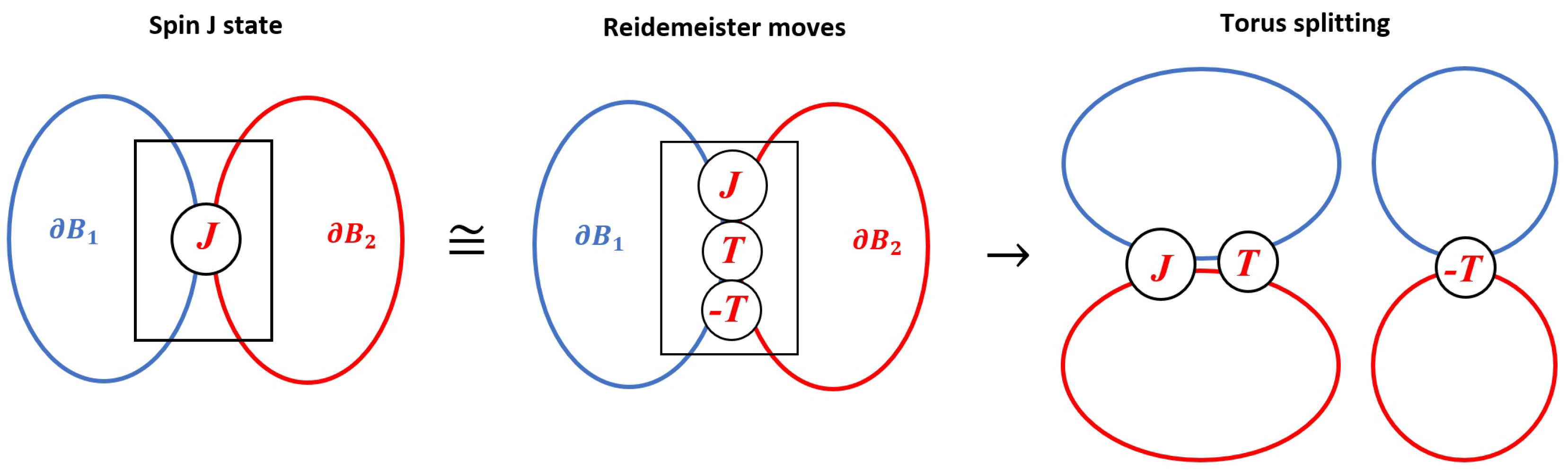
Next, using the different representations for the quantum phase introduced in Section 3, we introduce a haptic model of maximally entangled Bell states using knot theory. Similar to Section 2, we consider a homotopy on which is perpendicular to the direction of the state vector on the Bloch sphere as shown in Figure 8 in the -realm, compare Figure 3 for the Heegard splitting in the -realm. For , the phase is constant, for the phase vanishes in the -realm due to antisymmetry. We start with the knot structure ignoring inner twists. Obviously, for a constant phase, the knot structure is trivial, as shown in Figure 9 (middle part). However, using Type-2 Reidemeister moves, it becomes evident that a constant phase can also be viewed e.g., as the phase of the combination of two orthogonal qubits.
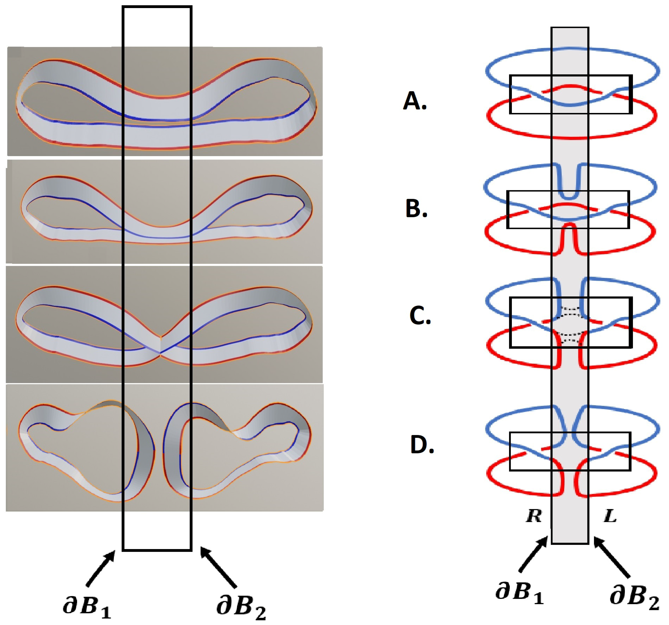
Now, we discuss the transition of the entangled state with constant phase to a pair of qubits in the paper strip model including twists, see Figure 10. Here, we restrict to the case near the boundaries and , where we suppose that the quantum phases ranging from and those ranging from are glued together. The general case within the bulk of and will be discussed in Section 6. The Reidemeister move shown in Figure 9 correspond to the insertion of one R and one L twist by a single of one part of the paper strip, see Figure 10A. In Figure 10B, the rotated part meets the paper strip at an arbitrary, different position. Particle creation can be visualized as a transition which we call a : Angular momentum conservation implies that the total number of twists in the initial state in the -realm is the same as the total number of twists in the final state, . This requirement uniquely defines the torus splitting, where two cuts arise as shown in Figure 10C and the phase is rejoined as shown in Figure 10D.
In the example shown in Figure 10, , and . Before the splitting, a distinction between both particles is impossible, as shown in Figure 10A–C. In this sense, the entangled state is single quantum state.
Taking the partial trace, the entangled state is reduced to a mixed state
Please note that this result is independent of the choice of basis. Topologically, this corresponds to the splitting of both qubits; however, the association of both parts to the particles observed from Alice (A) of Bob (B) can emerge in two different permutations, compare to Figure 10D. This leads to observation of with probability , and with probability by Alice and Bob.
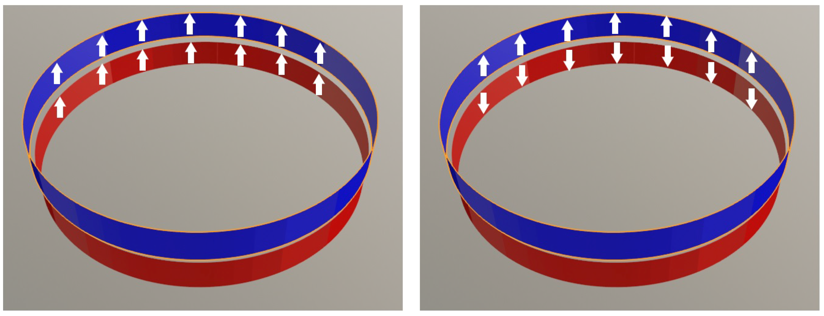
Next, we discuss the case . As shown in Figure 11, the constant phase at boundary and in the -realm does not vanish, but is constant. In the -realm, both parts can be combined either in constructive or in destructive interference. In the latter case, the amplitude is zero in the -realm. The knot structure and the creation mechanism of the qubits remains the same as for the case of discussed above, and shown in Figure 10.
In this example, the number of inner twists also remains constant, as two fermions are created with inner twists. Note however that the total number of inner twists may change, since bosons and fermions differ by twist due to the mechanism shown in Figure 7.
6. A Haptic Model of Gauge Symmetries
6.1. Minimal Interaction
In what follows, we will restrict to -gauge symmetry. In Figure 2, we may think that due to symmetry breaking, two degrees of freedom are frozen out and become immobile (This idea was first proposed by Christian Klein-Bösing.). We consider the phase of an arbitrary quantum state with J twists on a given homotopic loop. Gauge invariance just amounts to the fact that an arbitrary number of topologically equivalent quantum phases exist which all map to the same observable state in the -realm, compare Figure 3. In particular, we may include additional twists as , see Figure 12. Let be an additional -phase factor in the ()-realm with T additional twists.
The insertion of this additional phase leads for the momentum operator to
Obviously, gauge invariance in valid. It is well known that the requirement of gauge invariance leads to so-called minimal interaction, which is the cornerstone of the standard model of particle physics. We here discuss the key ideas in the non-relativistic case; the generalization to the relativistic case is straightforward and can be found in textbooks [10]. We introduce a generalized momentum operator which is required to obey gauge invariance as follows:
This change of the momentum operator can be realized by the introduction of the gauge field . With
gauge invariance is maintained if the gauge field compensates for the transformation of the phase of the wave function as
This is the -version (with explicit prefactor) of the -gauge transformation defined in (7). As shown in Figure 12, the change of the phase of the wave function and of the gauge field
just corresponds to T rotations of the paper strip, leading to a homotopically equivalent quantum phase with twists. Particle corresponds topologically to torus splitting, where two cuts separate the quantum phases with the twists and . Then, is the phase of the wave function with twists, and corresponds to the compensating phase of the gauge field with twists. Please note that the situation for and exactly corresponds to the quantum phase of two entangled Bell states, compare Figure 10.
6.2. Selection Rules
As an application, we discuss transition amplitudes for bound electrons in the hydrogen atom. We want to demonstrate the power of the paper strip model for a topological understanding of gauge interaction. Using Figure 12, we can make predictions on allowed and forbidden transitions, i.e., on selection rules in the atom. Consider an electron in the quantum state with . As the photon has , we have to deform the quantum phase by rotating () the closed paper strip twice, see Figure 13 and Figure 14A,B. Note that, when orbital angular momentum is included, is also possible. After particle creation (corresponding in the paper strip model to the torus splitting, Figure 14C,D), the remaining phase of the electron must contain twists, which cannot be achieved in the state with . For this reason, the fact that the state is metastable can be modeled using the paper strip model. On the other hand, the state can decay to a state with . Due to the minimal interaction, the entangled state
will emerge, which due to decoherence will decay to a mixture of left-circular polarized light with an electron in the state , or right-circular polarized light with an electron in the state , see Figure 13. Please note that we come to this prediction without explicit calculation, just by considering the topology of the quantum phase.
It is fascinating to see that the quantum phase does not change due to the interaction - the constant phase of the state is homotopically equivalent to the quantum phase of the entangled state and remains constant, showing that it is truly a interaction. Only after reduction to a mixed state, similar to the simple two-qubit model described in Section 5, by ignoring one of the possible realizations or , the phase is changed. Formally, this is described by taking the partial trace over both possible polarizations of the photon
In some sense, interaction can be viewed as ignorance of the remaining part of the entangled state. Physically, this may be achieved by decoherence due to interaction of the photon with the environment, which may be modeled as a heat bath.
It is instructive to compare the mathematical formalism necessary for the derivation of transition rules to the ansatz based on the paper strip model. The minimal interaction scheme leads in non-relativistic quantum physics to the Hamiltonian
Gauge invariance can be proven using (23) and
The free Hamiltonian describes the bound electron in the hydrogen atom; and describes the interaction with the gauge field as
For the evaluation of transition amplitudes, we must consider the matrix elements between some initial and final state, defined by
For electromagnetic transitions, the relevant interaction is given by
with
The creation and annihilation operator fulfil the commutation relation
Here, described the polarization of the photon created. In the -realm, all polarization states can be described on the Bloch sphere. Here, a subtle remark is in order. Since the photon is massless, no longitudinal modes emerge. For this reason, the degree of freedom of polarization is effectively two-dimensional. In contrast to spin, however, no sign change after a -rotation emerges.
In view of Fermi’s golden rule, only those modes of the gauge field with are relevant for the transition. Thus, we may write to the interaction operator relevant for the creation and emission of a photon as
The multipole expansion of leads all possible electric and magnetic transitions with creation of a single photon with . For leading order, the matrix element is given by
Here, we used . From this expression, the selection rule and can be derived [14], as anticipated using the paper strip model. Using similar arguments, the higher multipole transitions can also be modeled with the paper strip model.
Finally, we want to comment on the role of the creation and annihilation operators within the paper strip model. As obvious from Figure 12, torus splitting and torus merging correspond to the creation and annihilation of particles. Therefore, the expansion of the unitary time development operator describes multi-photon processes, where those terms containing involve k torus splittings. Much the same as higher order terms in the multipole expansion for , see Equation (36), terms with are suppressed by higher powers in the fine structure constant .
6.3. Feynman Diagrams and Entanglement
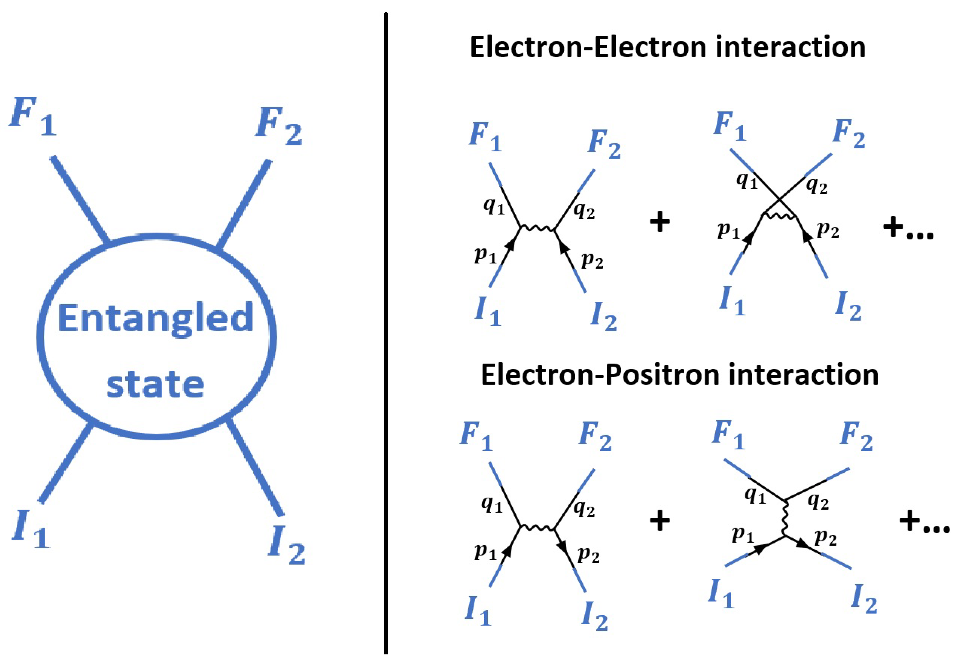
As a final example, we discuss the relation between Feynman diagrams and the paper strip model. We consider the interaction between two ingoing particles , which after the interaction asymptotically lead to the final particles . To be specific, we consider two examples: electron-electron and electron-positron interaction ( For simplicity, we do not discuss the creation of new particles, although this would be possible as straightforward generalization of the arguments given in the last section, including one additional torus splitting for each particle). In both cases, we denote by the four-momentum of the ingoing particles, and by those of the outgoing particles. The conservation of energy and momentum reads
with . The interaction can be described by generalizing the -gauge invariance from non-relativistic quantum physics to quantum field theory. The resulting theory is called QED. We want to emphasize that interaction and entanglement are closely related, as we will show in what follows. Let us denote the transition amplitude to the final state as . If we exchange the four-momentum of the final particles, the matrix element is given by .
In case of the scattering of two electrons, both contributions lead to an indistinguishable result. Thus, the total amplitude is given as a superposition
Finkelstein and Rubinstein have shown that the exchange of two particles is homotopically equivalent to a rotation of one of the particles in the -realm [15]. As corresponds to this -rotation, the exchange of two fermions leads to a minus sign. Indeed, the result is an entangled state, since the difference of both permutations lead to superposition of product states.
In case of electron-positron scattering, exchange of the electron and positron lead to a different final state, thus no superposition emerges. Instead, there exist different types of amplitudes, which we call scattering and annihilation processes, see Figure 15. The result is again an entangled state,
Since the interaction of two particles of spin is discussed, we conclude that the entangled state can be described as shown in Figure 10. Indeed, after the Reidemeister move, we may view the knot either as a composition of two spin particles, or as a gauge field with two twists. Since all these configurations are topologically equivalent, the question whether virtual particles ‘exist’ or not boils down to the question whether the infinite number of possible Reidemeister moves ‘exist’ or not: Of course they do, but the knot structure is only changed when a torus splitting divides the knot structure, which corresponds to particle creation. Thus, the quantum phase of the scattering and the annihilation processes cannot be separated from each other, since in the entangled state, all these configurations coexist as homotopically equivalent realizations.
It is instructive to consider the phase of the entangled state also in the -realm. The corresponding operations with Jones polynomials are derived in Appendix A. In Figure 16A), we show the constant phase of the entangled state of two spin -particles (e.g., two electrons, or one electron and one positron) with total for momentum . Homotopically equivalent is b.), which can also be viewed as gauge interaction, see Figure 12 with . In contrast to the Feynman diagrams, which separate the different amplitudes, in the paper strip model, all possible contributions are contained as homotopically equivalent configurations in a single quantum phase of the entangled state.
In the -realm, the torus splitting can be described in two separate steps. The configuration c.) after one split is not an observable, as it does not meet the requirement on inner twists for Hopf mapping discussed in Section 3. Instead, only after a second split as shown in d.), two Dirac belts emerge, with opposite inner twisting (e.). The four-momentum is distributed among them such that the sum is .
Of course, for explicit calculations, Feynman diagrams are the (mathematical) tool to be addressed. However, a literal reading of single Feynman diagrams as certain physical processes occurring in space time can lead to misconceptions [16]. The advantage of the paper strip model is thus conceptual: The fascinating properties of entanglement can be grasped better, since the intermediate state be divided into separate processes. Rather, the close relation between interaction and entanglement becomes evident.
7. Discussion
Our key idea can be explained just by considering the paper strip model of a constant phase shown in Figure 11. By rotating one piece of the paper strip, the total number of twists does not change. Indeed, T rotations lead to twists in the closed paper strip. For , we obtain a model of Bell states as shown in Figure 10, Section 5, and a model of scattering amplitudes as shown in Figure 14, Section 6.
For , we obtain a model of emission and absorption of a spin 1 gauge boson (a photon), as shown in Figure 14, Section 6. The twists in the -realm are related to inner twists and knots in the -realm as shown in Figure 6. For example, for the rotation, four inner twists are created as shown in Figure 16 in the -realm. Please note that inner twists can be undone by the Dirac belt trick (This version of the Dirac belt trick is shown in https://vimeo.com/62228139).
For the -gauge field emerging in the Chern–Simons action given by Equation (5), Section 4, the number of inner twists is related to the winding number as . Just by adapting the argument leading to the haptic model of gauge symmetry in the -realm shown in Figure 12 to the situation in the -realm, we can derive sum rules. Let us start with a paper strip with zero inner twists. By rotating times, inner twists emerge in the gauge field. Therefore, inner twists emerge in the wave function (e.g., of the quark field) interacting with the gauge field. As shown in Figure 7, the standard mapping (11) related to inner twists in the gauge field necessarily leads to one spin zero mode field with inner twists. More details on sum rules will be discussed elsewhere.
Using the paper strip model in the -realm and the corresponding paper strip where the parts and are glued together in the -realm, the close relation between the different applications ranging from entanglement to minimal interaction becomes obvious. However, the mathematical formalism looks quite different and the intimate relations are not directly visible in the equations. For this reason, we think that the paper strip model may have particular merits for science education.
Author Contributions
Conceptualization, S.H.; investigation, S.H. and M.U.; writing–review and editing, M.U.; visualization, M.U.
Funding
This research received no external funding.
Conflicts of Interest
The authors declare no conflict of interest.
Appendix A
Appendix Jones Polynomials and Inner Twists
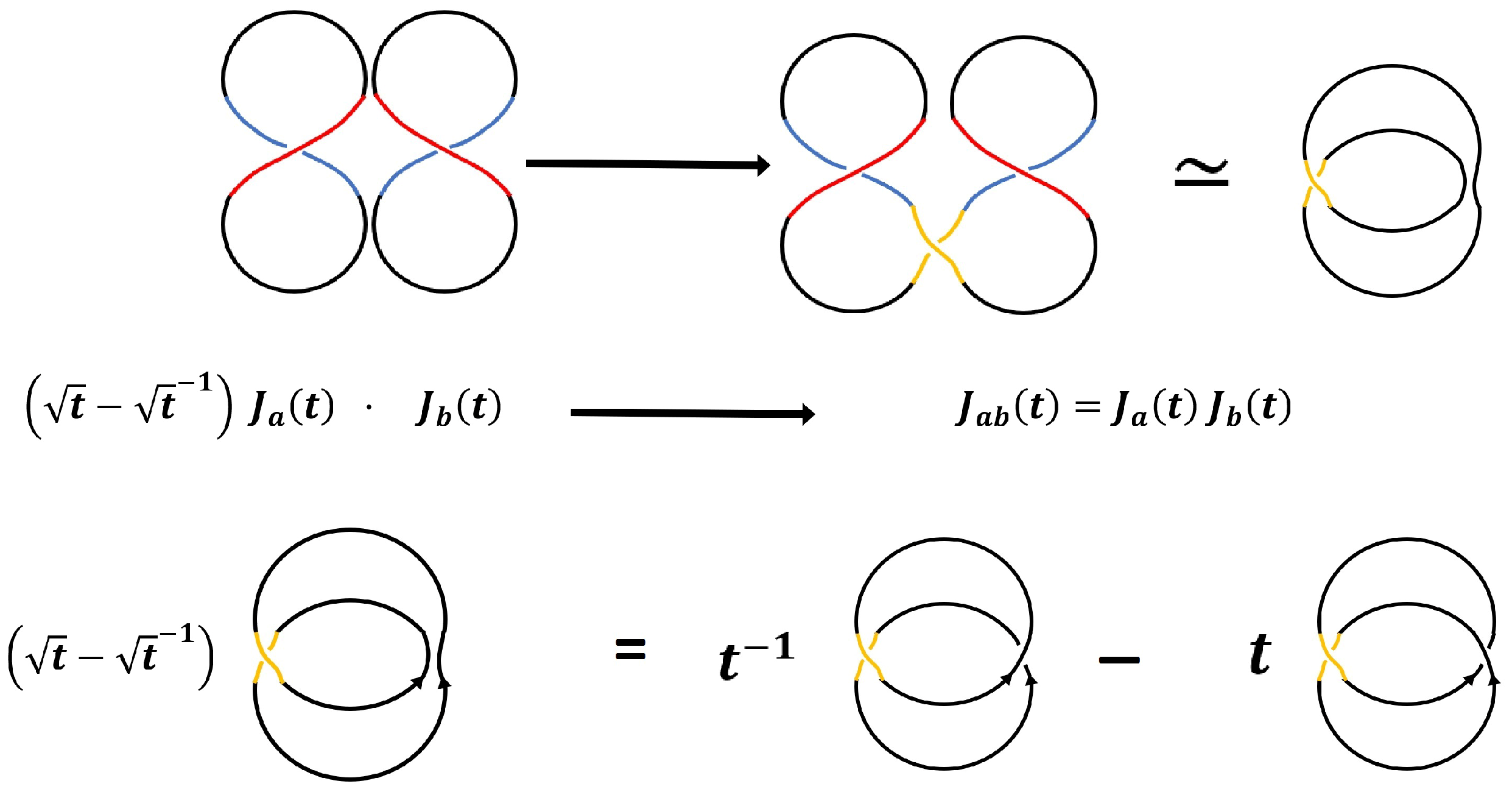
In this appendix, we calculate the Jones polynomials relevant for the torus splitting (torus merger) in the -realm shown in Figure 15. In general, the Jones polynomial of the combination of two knots is given by with . If both knots are connected as shown in Figure A1, the Jones polynomial of the resulting knot (or link) is given by the product . For the case relevant for entanglement as shown in Figure 15, describe spin particles with . Please note that inner twists are not addressed by the Jones polynomial. Using the recursion relation [3]
we find
with and . This is, of course, the right answer, but does not describe inner twists.
Figure A1.
Calculation of Jones polynomials for the torus splitting described in the main text (Figure 16).
Figure A1.
Calculation of Jones polynomials for the torus splitting described in the main text (Figure 16).

As discussed in the main text, additionally to the knot structure, inner twists must be taken into account. For the situation shown in Figure 16B), with the inner twists the Dirac belt trick can be performed. After the torus splitting , we obtain a pair with twists, shown in Figure 16D). In the -realm, this corresponds to two Möbius bands with opposite chirality with .
References
- Bonesteel, N.E.; Hormozi, L.; Zikos, G.; Simon, S.H. Braid group representation on quantum computation. Phys. Rev. Lett. 2005, 95, 14. [Google Scholar] [CrossRef] [PubMed]
- Aziz, R.; Muchtadi-Alamsyah, I. Braid group representation on quantum computation. AIP Conf. Proc. 2015, 1677. [Google Scholar] [CrossRef]
- Heusler, S.; Ubben, M. Modelling spin. Eur. J. Phys. 2018, 39, 065405. [Google Scholar] [CrossRef]
- Heusler, S.; Ubben, M. A Haptic Model for the Quantum Phase of Fermions and Bosons in Hilbert Space Based on Knot Theory. Symmetry 2019, 11, 426. [Google Scholar] [CrossRef]
- Dür, W.; Heusler, S. What we can learn about quantum physics from a single qubit. arXiv 2013, arXiv:1312.1463. [Google Scholar]
- Dür, W.; Heusler, S. Visualization of the Invisible: The Qubit as Key to Quantum Physics. Phys. Teach. 2014, 52, 489–492. [Google Scholar] [CrossRef]
- Nikolai, S. Lectures on the topology of 3-manifolds. An introduction to the Casson invariant. In de Gruyter Textbook; de Gruyter: Berlin, Germany, 2012; ISBN 9783110250350. [Google Scholar]
- Kauffmann, L. Knoten-Diagramme, Zustandsmodelle, Polynominvarianten. In Spektrum der Wissenschaften; Spektrum: Heidelberg, Germany, 1995; ISBN 9783860252321. [Google Scholar]
- Wheeler, N. Spin matrices for arbitrary spin. In Lecture Notes; Read College Physics Department: Portland, Oregon, 2000. [Google Scholar]
- Coleman, S. Selected Erice Lectures; Cambridge University Press: Cambridge, UK, 1999; pp. 288–290. [Google Scholar]
- Witten, E. Quantization of Chern-Simons gauge theory with complex gauge group. Commun. Math. Phys. 1991, 1, 29–66. [Google Scholar] [CrossRef]
- Horodecki, R.; Horodecki, P.; Horodecki, M.; Horodecki, K. Quantum entanglement. Rev. Mod. Phys. 2009, 81, 865–942. [Google Scholar] [CrossRef]
- Dür, W.; Heusler, S. Was man von zwei Qubits über Quantenphysik lernen kann: Verschränkung und Quantenkorrelationen. PhyDid A-Phys. Und Didakt. Sch. Und Hochsch. 2014, 13, 11–34. [Google Scholar]
- Sakurai, J.J. Modern Quatum Mechanics; Addison Wesley: Boston, MA, USA, 1993. [Google Scholar]
- Finkelstein, D.; Rubinstein, J. Connection between spin, statistics, and kinks. J. Math. Phys. 1968, 9, 1762–1779. [Google Scholar] [CrossRef]
- Passon, O. On the interpretation of Feynman diagrams, or, did the LHC experiment observe H → γγ. Eur. J. Philos. Sci. 2019, 9, 20. [Google Scholar] [CrossRef] [Green Version]
Figure 1.
Quantum tomography: For an ensemble of identical qubits, successive measurements lead to a random pattern with probabilities for ‘black’ ( eigenvalues) or ‘white’ ( eigenvalues) in the direction, respectively. With as probability for ‘black’, and as probability for ‘white’, the relation holds. Here, is the density matrix of the single qubit.

Figure 2.
The operation of the quaternions on the Dirac belt in the -realm. Note that these operations lead to inner twists of the Dirac belt. In particular, for operation leads to two inner twists.
Figure 2.
The operation of the quaternions on the Dirac belt in the -realm. Note that these operations lead to inner twists of the Dirac belt. In particular, for operation leads to two inner twists.

Figure 3.
Left: Heegaard splitting of , Right: Hopf mapping to the Bloch sphere. In , a homotopic loop is considered ranging from , which is mapped to a great circle traversed on the Bloch sphere . The Dirac belt describing the quantum phase on the homotopic loop in is equivalent to a Möbius strip when the parts and separated in are ‘glued together’, [see also Figure 4]. Superposition of right- and left-twisted Möbius strips leads to a node on the Bloch sphere. The antipode of this node is called ‘direction of the spin’, describing the direction of maximal amplitude.

Figure 4.
The node on the Bloch sphere [in this case, the node at arises due to superposition of the quantum phases ]. In the -realm, an infinite number of homotopically equivalent quantum phases in arise which all map to the great circle . The superposition on the Bloch sphere translates to a superposition of Dirac belts.

Figure 5.
Representation of the superposition state on the Bloch sphere (-realm). Positions × of nodes are antipodes to the direction of . The superposition of the qubits changes the position of the direction of the spin, which in turn changes the position × of the node. The relation between nodes on the Bloch sphere and knots in Hilbert space are shown in Figure 4.

Figure 6.
For spin j-states, nodes arise on the Bloch sphere which may be described as a complex function in the stellar representation. The corresponding knot structure in the -realm is described by the Jones polynomial . Additionally, the quantum phase has inner twists (bosons), or inner twists (fermions), respectively, denoted by (+).

Figure 7.
Left: Double copy of inner twists, describing a boson with spin . Right: By joining the two pieces to a fermionic knot, two additional inner twists arise, leading to a knot with .
Figure 7.
Left: Double copy of inner twists, describing a boson with spin . Right: By joining the two pieces to a fermionic knot, two additional inner twists arise, leading to a knot with .

Figure 8.
Due to the interaction with , the initial state becomes the entangled Bell state . We consider the homotopic loop perpendicular to the -direction.
Figure 8.
Due to the interaction with , the initial state becomes the entangled Bell state . We consider the homotopic loop perpendicular to the -direction.

Figure 9.
Using transitions to homotopically equivalent knots similar to Type-2 Reidemeister moves in the -realm, the constant phase can also be viewed as a combination of two qubits or . Since both possibilities are indistinguishable, the superposition emerges, which is an entangled state. After taking the particle trace, a mixed state arises. The latter result is basis-independent.

Figure 10.
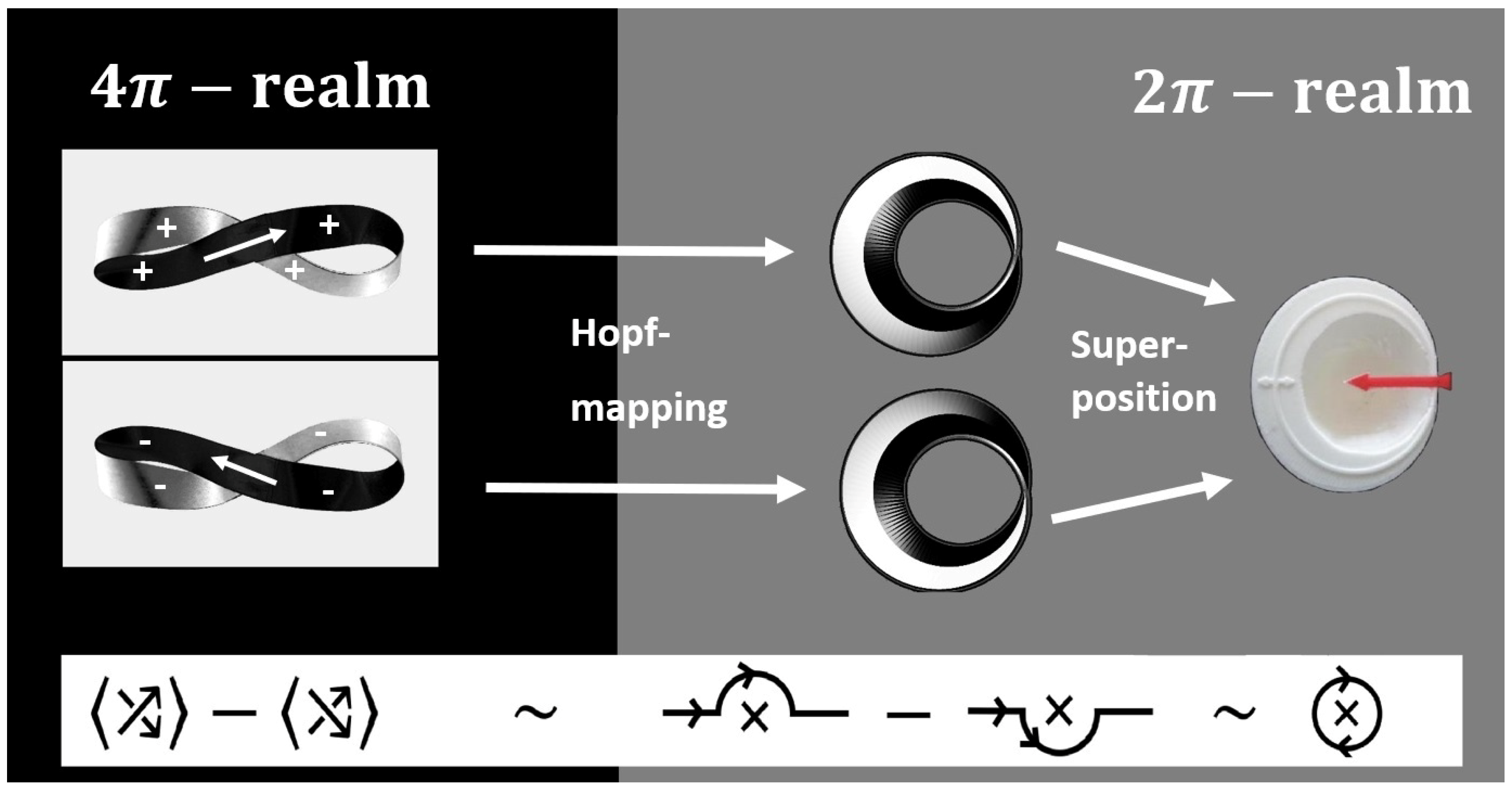
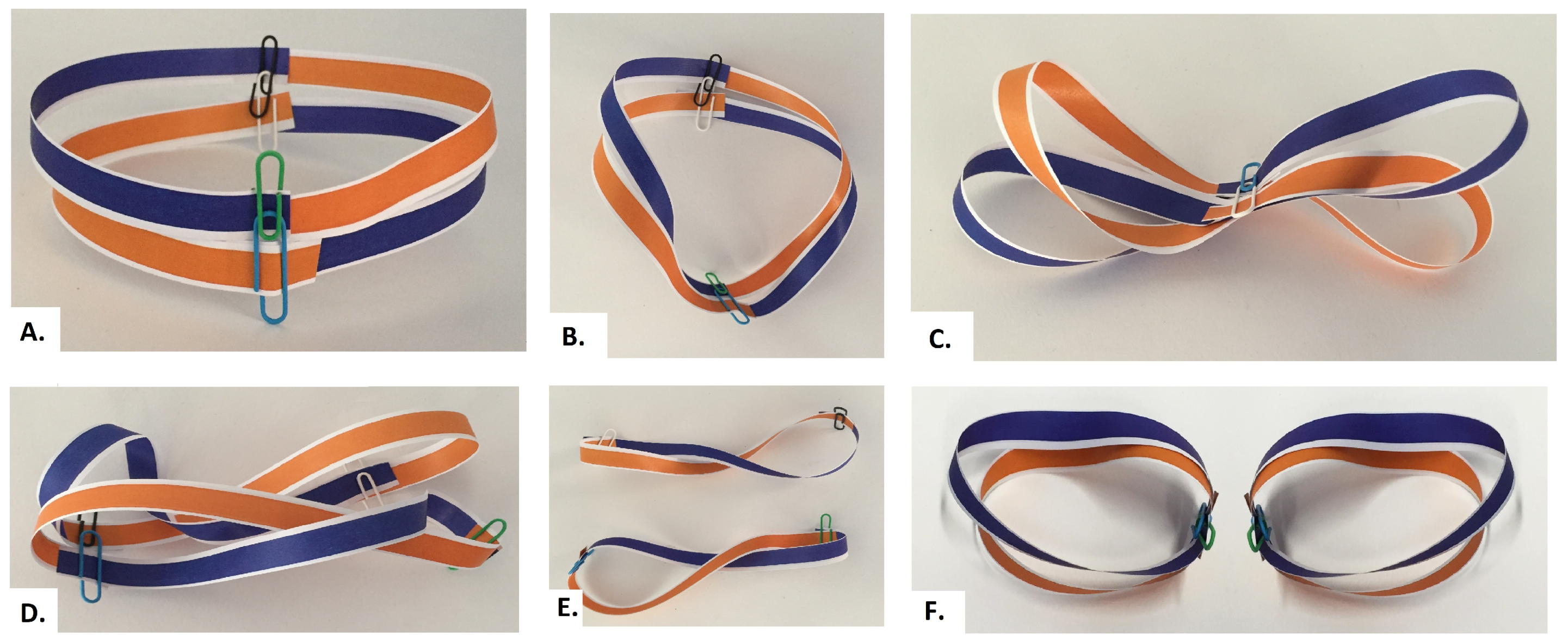
Paper strip model of the interaction of two qubits: The entangled state is described by one common state with one quantum phase. By rotating the phase once and cutting into two pieces, two separate particles with left- and right twists arise. Here, we use the model of the paper strip near the boundary, where the phases and are glued together. The general homotopy in the -realm is shown in Section 6.3.
Figure 10.
Paper strip model of the interaction of two qubits: The entangled state is described by one common state with one quantum phase. By rotating the phase once and cutting into two pieces, two separate particles with left- and right twists arise. Here, we use the model of the paper strip near the boundary, where the phases and are glued together. The general homotopy in the -realm is shown in Section 6.3.

Figure 11.
In the -realm, the constant phase in can superpose constructively (symmetric wave function) or destructively (anti symmetric wave function) with the constant phase in . The situation on the Bloch sphere in the -realm is shown in Figure 8.
Figure 11.
In the -realm, the constant phase in can superpose constructively (symmetric wave function) or destructively (anti symmetric wave function) with the constant phase in . The situation on the Bloch sphere in the -realm is shown in Figure 8.

Figure 12.
Paper strip model of minimal interaction: The insertion of additional twists is compensated by a gauge field. Only after a torus splitting, the gauge field with twists is separated from the original particle, which then has twists due to the gauge interaction.
Figure 12.
Paper strip model of minimal interaction: The insertion of additional twists is compensated by a gauge field. Only after a torus splitting, the gauge field with twists is separated from the original particle, which then has twists due to the gauge interaction.

Figure 13.
The quantum phase of the state is homotopically equivalent to , see also Figure 9. The entangled state decays into a mixed state due to interaction of the photon with the environment.
Figure 13.
The quantum phase of the state is homotopically equivalent to , see also Figure 9. The entangled state decays into a mixed state due to interaction of the photon with the environment.

Figure 14.
Paper strip model of the quantum phase of the decay in the -realm. If is associated with the right-circular polarized photon, the described the quantum phase of the electron in the state . With probability, the roles of the pieces and are interchanged, see Figure 13.
Figure 14.
Paper strip model of the quantum phase of the decay in the -realm. If is associated with the right-circular polarized photon, the described the quantum phase of the electron in the state . With probability, the roles of the pieces and are interchanged, see Figure 13.

Figure 15.
Leading-order Feynman diagrams for electron-electron and electron-positron interaction. In view of entanglement, a direct interpretation of Feynman diagrams in space time is impossible. The quantum phase of the entangled state can be modeled in the -realm as shown in Figure 10, and in the -realm as shown in Figure 16.

Figure 16.
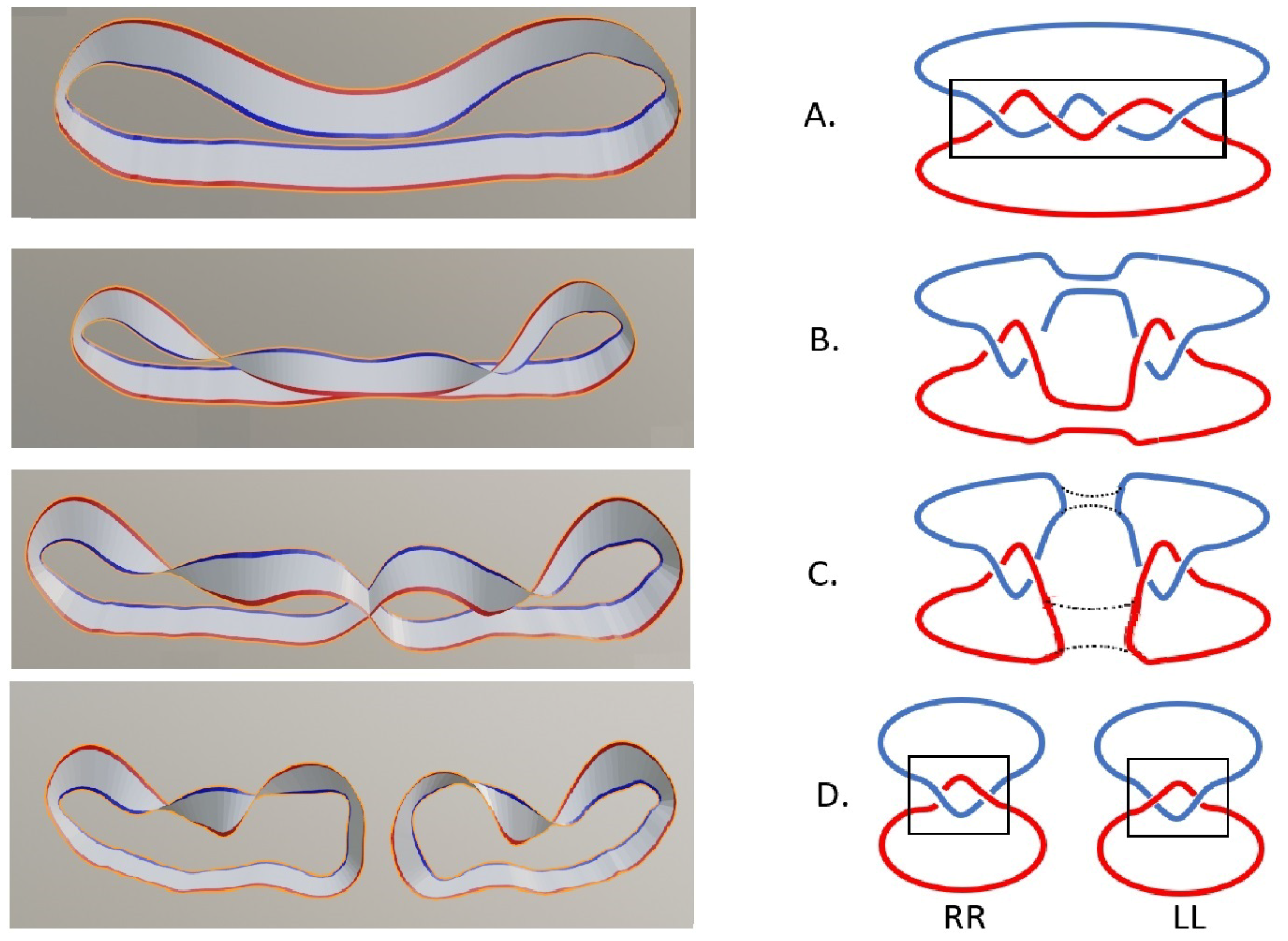
Haptic model of the quantum phase of an entangled pair of qubits in the -realm. Here, we consider any homotopy in the bulk of and in the Heegaard splitting, see Figure 3. After Hopf mapping, the pieces and from and are ‘glued together’, leading to the description in the -realm as shown in Figure 10. As discussed in the text, we associate with the two qubits either a pair of electrons, or an electron-positron pair. (A) The constant phase, see also Figure 11. (B) One rotation leads to a homotopically equivalent configuration, which can be seen as a pair of entangled spin particles, see also Figure 10A. Due to the homotopic equivalences shown in Figure 9, we may view this quantum state also a combination of two spin particles with a (virtual) gauge particle. (C) Encounter of the quantum phases, see also Figure 10B. (D) First splitting of the quantum phase in the -realm, see also Figure A1 for the corresponding Jones polynomials. This configuration cannot be mapped to the -realm. (E) Second splitting of the quantum phase in the -realm. The situation in the -realm, where both splitting are combined to one torus splitting is shown in Figure 10C,D. (f) Quantum phase of two distinguishable spin particles in the -realm. The inner twists in the Dirac belts have opposite sign, i.e., and .
Figure 16.
Haptic model of the quantum phase of an entangled pair of qubits in the -realm. Here, we consider any homotopy in the bulk of and in the Heegaard splitting, see Figure 3. After Hopf mapping, the pieces and from and are ‘glued together’, leading to the description in the -realm as shown in Figure 10. As discussed in the text, we associate with the two qubits either a pair of electrons, or an electron-positron pair. (A) The constant phase, see also Figure 11. (B) One rotation leads to a homotopically equivalent configuration, which can be seen as a pair of entangled spin particles, see also Figure 10A. Due to the homotopic equivalences shown in Figure 9, we may view this quantum state also a combination of two spin particles with a (virtual) gauge particle. (C) Encounter of the quantum phases, see also Figure 10B. (D) First splitting of the quantum phase in the -realm, see also Figure A1 for the corresponding Jones polynomials. This configuration cannot be mapped to the -realm. (E) Second splitting of the quantum phase in the -realm. The situation in the -realm, where both splitting are combined to one torus splitting is shown in Figure 10C,D. (f) Quantum phase of two distinguishable spin particles in the -realm. The inner twists in the Dirac belts have opposite sign, i.e., and .

© 2019 by the authors. Licensee MDPI, Basel, Switzerland. This article is an open access article distributed under the terms and conditions of the Creative Commons Attribution (CC BY) license (http://creativecommons.org/licenses/by/4.0/).
Share and Cite
MDPI and ACS Style
Heusler, S.; Ubben, M. A Haptic Model of Entanglement, Gauge Symmetries and Minimal Interaction Based on Knot Theory. Symmetry 2019, 11, 1399. https://0-doi-org.brum.beds.ac.uk/10.3390/sym11111399
AMA Style
Heusler S, Ubben M. A Haptic Model of Entanglement, Gauge Symmetries and Minimal Interaction Based on Knot Theory. Symmetry. 2019; 11(11):1399. https://0-doi-org.brum.beds.ac.uk/10.3390/sym11111399
Chicago/Turabian StyleHeusler, Stefan, and Malte Ubben. 2019. "A Haptic Model of Entanglement, Gauge Symmetries and Minimal Interaction Based on Knot Theory" Symmetry 11, no. 11: 1399. https://0-doi-org.brum.beds.ac.uk/10.3390/sym11111399
Note that from the first issue of 2016, this journal uses article numbers instead of page numbers. See further details here.