Modified Power-Symmetric Distribution


1
Department of Quantitative Methods in Economics and TIDES Institute, University of Las Palmas de Gran Canaria, 35017 Las Palmas de Gran Canaria, Spain
2
Departamento de Matemáticas, Facultad de Ciencias Básicas, Universidad de Antofagasta, Antofagasta 1240000, Chile
3
Centre for Actuarial Studies, Department of Economics, The University of Melbourne, Melbourne, VIC 3010, Australia
*
Author to whom correspondence should be addressed.
Symmetry 2019, 11(11), 1410; https://0-doi-org.brum.beds.ac.uk/10.3390/sym11111410
Submission received: 2 October 2019
/
Revised: 8 November 2019
/
Accepted: 13 November 2019
/
Published: 15 November 2019
(This article belongs to the Special Issue Symmetric and Asymmetric Distributions: Theoretical Developments and Applications)
Abstract
:In this paper, a general class of modified power-symmetric distributions is introduced. By choosing as symmetric model the normal distribution, the modified power-normal distribution is obtained. For the latter model, some of its more relevant statistical properties are examined. Parameters estimation is carried out by using the method of moments and maximum likelihood estimation. A simulation analysis is accomplished to study the performance of the maximum likelihood estimators. Finally, we compare the efficiency of the modified power-normal distribution with other existing distributions in the literature by using a real dataset.
1. Introduction
Over the last few years, the search for flexible probabilistic families capable of modeling different levels of bias and kurtosis has been an issue of great interest in the field of distributions theory. This was mainly motivated by the seminal work of Azzalini [1]. In that paper, the probability density function (pdf) of a skew-symmetric distribution was introduced. The expression of this density is given by
where is a symmetric pdf about zero; is an absolutely continuous distribution function, which is also symmetric about zero; and is a parameter of asymmetry. For the case where is the standard normal density (from now on, we reserve the symbol for this function), and is the standard normal cumulative distribution function (henceforth, denoted by ), the so-called skew-normal () distribution with density
is obtained. We use the notation to denote the random variable Z with pdf given by Equation (2). A generalization of the distribution is introduced by Arellano-Valle et al. [2] and Arellano-Valle et al. [3]; they study Fisher’s information matrix of this generalization. For further details about the distribution, the reader is referred to Azzalini [4]. Martínez-Flórez et al. [5] used generalizations of the distribution to extend the Birnbaum-Saunders model, and Contreras-Reyes and Arellano-Valle [6] utilized the Kullback–Leibler divergence measure to compare the multivariate normal distribution with the skew-multivariate normal.
One of the main limitations of working with the family given by Equation (1) is that the information matrix could be singular for some of its particular models (see Azzalini [1]). This might lead to some difficulties in the estimation, due to the asymptotic convergence of the maximum likelihood (ML) estimators. To overcome this issue, some authors (see Chiogna [7] or Arellano-Valle and Azzalini [8]) have used a reparametrization of the model to obtain a nonsingular information matrix. However, this methodology cannot be extended to all type of skew-symmetric models which suffers of this convergence problem. On the other hand, the family of power-symmetric () distributions does not have this problem of singularity in the information matrix (see, Pewsey et al. [9]). The pdf of this family of distribution is given by
where is itself a cumulative distribution function (cdf) and is the shape parameter. For the particular case that , the power-normal () distribution is obtained, with density given by
For some references where this family is discussed, the reader is referred to Lehmann [10], Durrans [11], Gupta and Gupta [12], and Pewsey et al. [9], among other papers. Other extensions of this model are given in Martínez-Flórez et al. [13], where a multivariate version from the model is introduced; also, Martínez-Flórez et al. [14] carried out applications by using regression models; finally, Martínez-Flórez et al. [15] examined the exponential transformation of the model, and Martínez-Flórez et al. [16] examined a version of the model doubly censored with inflation in a regression context. Truncations of the distribution were considered by Castillo el al. [17].
In this paper, a modification in the pdf of the probabilistic family is implemented to increase the degree of kurtosis. This methodology is later used to explain datasets that include atypical observations. Usually, this methodology is accomplished by increasing the number of parameters in the model.
The paper is organized as follows. In Section 2, first, we introduce the modified power symmetric distribution. Then, the particular case of the modified power normal distribution is derived. Some of the most relevant statistical properties of this model, including moments and kurtosis coefficient, are presented. Next, in Section 3, some methods of estimation are discussed. Later, a simulation study is provided to illustrate the behavior of the shape parameter. A numerical application where the modified power normal distribution is compared to the and distributions is given in Section 4. Finally, Section 5 concludes the paper.
2. Genesis and Properties of Modified Power-Normal Distribution
In this section, we introduce a new family of probability distributions. The idea is to make a transformation to a given probability density, as the skew-symmetric or power-symmetric distributions does. As there exists a certain resemblance between our formula (Equation (6)) and the formula for the power-symmetric distributions (Equation (3)), we agree to name these new distributions as modified power-symmetric distributions. From the standard normal distribution, we obtain the so-called Modified Power-Normal distribution. The main parameters and properties of this particular distribution will be studied throughout this work.
2.1. Probability Density Function
Definition 1.
Let Z be a continuous and symmetric random variable with cdfand pdf, wheredenotes a vector of parameters. We say that, a random variable, X, follows adistribution, denoted as, if its cdf is given by
and its pdf is given by
whereand.
Remark 1.
In the case, the transformation given by Equation (6) is the identity. That is, thedistribution foralways provides the input probability density function.
Thereforeforth, we proceed to examine the distribution, whose cdf is provided by
and whose pdf is given by
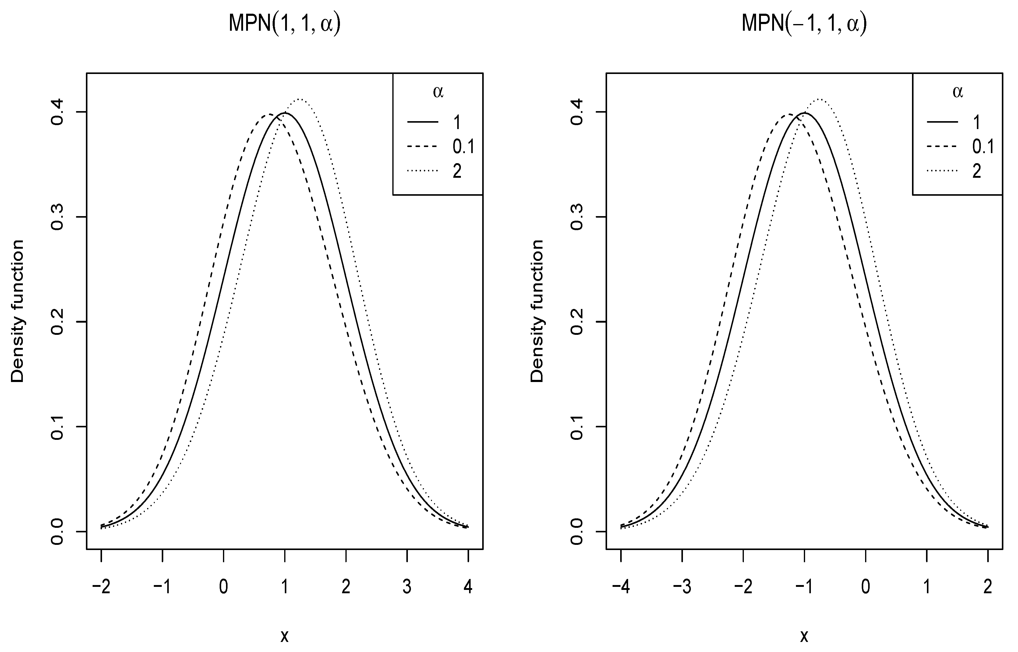
where , is the location parameter, is the scale parameter, and is the shape parameter. Hereafter, this will be denoted as . Figure 1 depicts some different shapes of the pdf of this model, for selected values of the parameter with and . The class of distributions is applicable for the change point problem, due to its favorable properties (see Maciak et al. [18]); moreover, the model can be utilized in calibration (see Peta [19]).
Remark 2.
Here,andare location and scale parameters of thedistribution, respectively. For the particular case, these are not only location and scale parameters but also the mean and standard deviation of the standard normal distribution.
2.2. Statistical Properties
2.2.1. Shape of the Density
The distribution exhibits a bell-shaped form, which can be symmetric or positively or negatively skewed depending on the value of the parameter . Now, we derive some analytical expressions that are useful to obtain approximations of modal values and inflection points of this model. In the following, it will be assumed that and .
Proposition 1.
The pdf ofhas a local maximum atand two inflection points atand, respectively, whereis the root of the equation
andandare two solutions of the equation
Proof.
The proof consists of simple derivatives of the function f. From the Equation (8), we calculate
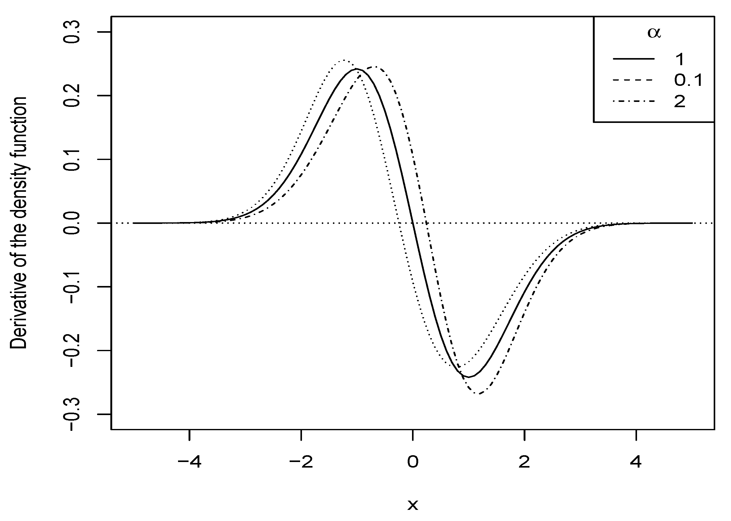
By setting Equations (9) and (10) to be equal to zero, the results are obtained after some algebra. Figure 2 displays the graph of the first derivative of , where it is observed that the maximum exists and it is unique. Therefore, the distribution is unimodal. □
2.2.2. Moments
Proposition 2.
The rth moments offorare given by
whereis defined as
Here,is the quantile function of the standard normal distribution.
Proof.
By using the change of variable , it follows that
□
Corollary 1.
The mean and variance of X are given by
respectively.
Corollary 2.
The skewness () and kurtosis () coefficients are, respectively, given by
Remark 4.
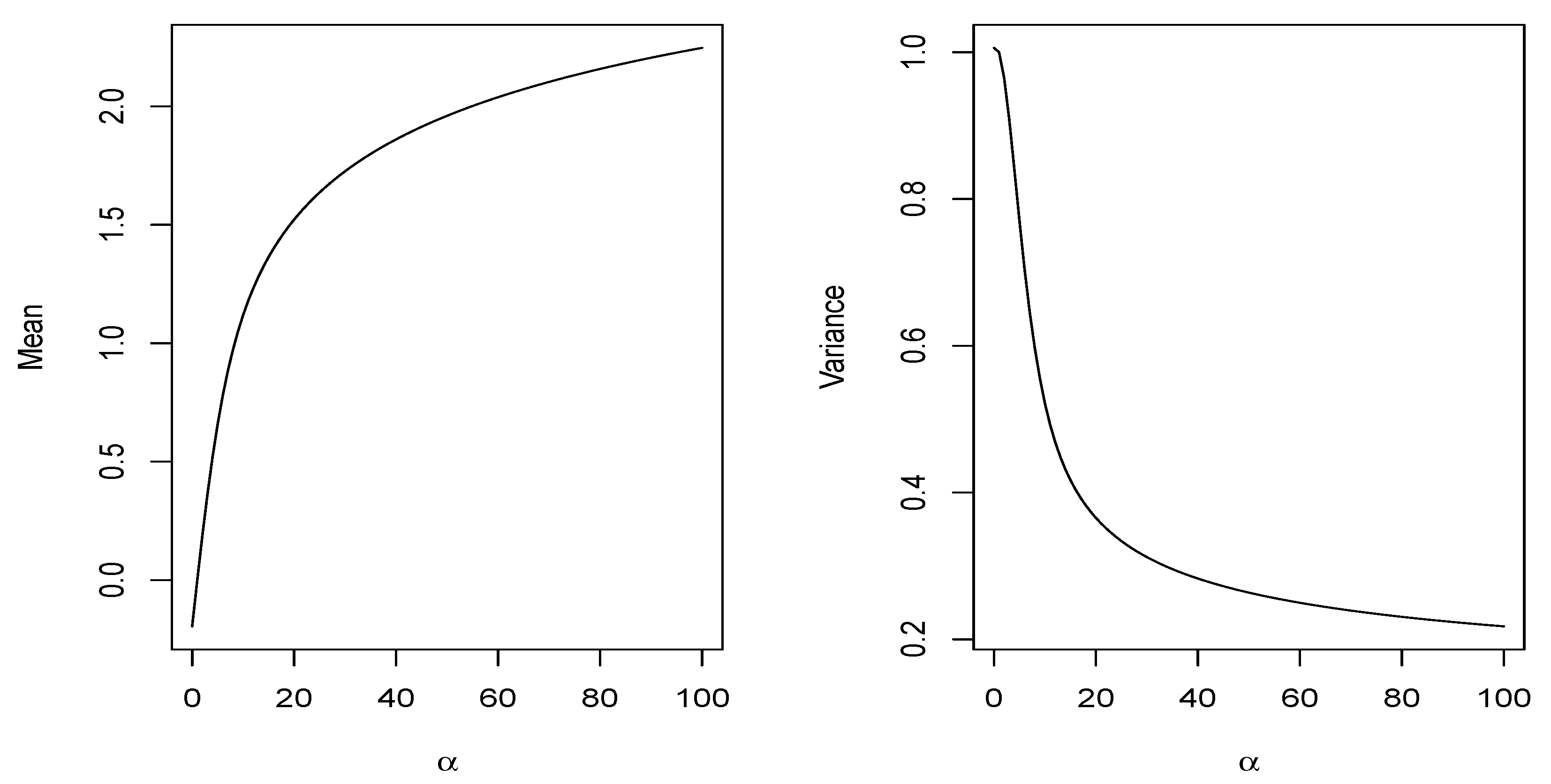
Observe that the integral in Equation (12) can be numerically approximated by using the built-in function integrate available in the software package R. Below, in Table 2 , some approximations of the mean and variance for the distribution for different values of α are displayed. Figure 3 illustrates the behavior of the and of the distribution for different values of α. It is observable that when α grows, the mean increases and the variance decreases.
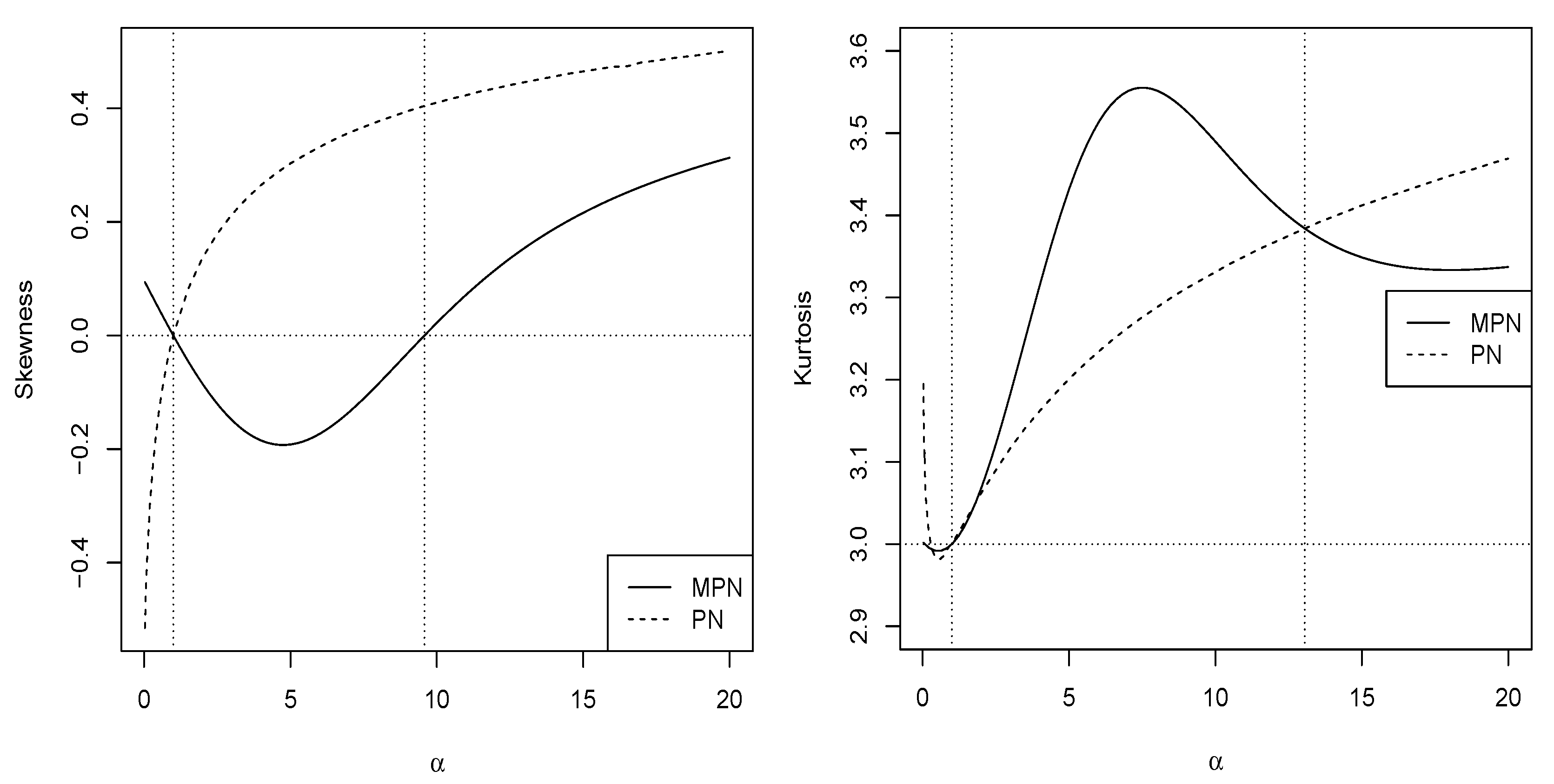
Figure 4displays the curves associated with the coefficients of skewness (left panel) and kurtosis (right) of theanddistributions. It is shown that, depending on the values of α, thedistribution exhibits equal, greater, or lesser values for these coefficients compared to themodel. In general, thedistribution has a smaller range of skewness than thedistribution. On the other hand, when, thedistribution has a greater kurtosis coefficient than themodel.
2.2.3. Stochastic Ordering
Stochastic ordering is an important tool to compare continuous random variables. It is well-known that random variable is smaller than random variable in stochastic ordering () if for all x, and in likelihood ratio order () if decreases with x.
Using Theorem 1.C.1 and Theorem 2.A.1 of Shaked and Shanthikumar [20], the above stochastic orders hold according to the following implications,
The proposition shows that the members of the family can be stochastically ordered according to parameters values.
Proposition 3.
Letand. If, thenand, therefore,.
Proof.
From the quotient of both densities, it follows that
is non-decreasing if and only if for , where
After some calculations, it is shown that
It is straightforward that for , then for . Therefore, is decreasing in x, and consequently . The other implication follows immediately from (13). □
3. Inference
In this section, parameters estimation for the distribution is discussed by using the method of moments and ML estimation. Additionally, a simulation analysis is carried out to illustrate the behavior of the ML estimators.
3.1. Method of Moments
The following proposition illustrates the derivation of the moment estimates of the distribution.
Proposition 4.
Letbe a random sample obtained from the random variable, then the moment estimatesforare given by
and
where, anddenote the sample mean, sample standard deviation and sample Fisher’s skewness coefficient respectively.
Proof.
As and are location and scale parameters respectively, the skewness coefficient does not depend on these parameters. Thus, the result in (15) is directly obtained from matching the sample skewness coefficient with population counterpart given in Corollary 2. In addition, by considering that , where , and again by equating sample mean and sample variance to the mean and variance respectively, it follows that
and
where satisfies expression (15). Then, (14) is obtained by solving the latter equations for and , respectively. □
3.2. Maximum Likelihood Estimation
For a random sample derived from the distribution, the log-likelihood function can be written as
where
The score equations are given by
where Solutions for these Equations (17)–(19) can be obtained by using numerical procedures such as Newton–Raphson algorithm. Alternatively, these estimates can be found by directly maximizing the log-likelihood surface given by (16) and using the subroutine “optim” in the software package [21].
3.3. Simulation Study
To examine the behavior of the proposed approach, a simulation study is carried out to assess the performance of the estimation procedure for the parameters , , and in the model. The simulation analysis is conducted by considering 1000 generated samples of sizes 100, and 200 from the distribution. The goal of this simulation is to study the behavior of the ML estimators of the parameters by using our proposed procedure. To generate , the following algorithm is used,
- Step 1: Generate
- Step 2: Compute
where , , and is the quantile function of the standard normal distribution. For each generated sample of the distribution, the ML estimates and corresponding standard deviation (SD) were computed for each parameter. As it can be seen in Table 3, the performance of the estimates improves when n and increases.
Fisher’s Information Matrix
Let us now consider and . For a single observation x of X, the log-likelihood function for is given by
The corresponding first and second partial derivatives of the log-likelihood function are derived in the Appendix A. It can be shown that the Fisher’s information matrix for the distribution is provided by
with the following entries,
where must be numerically computed.
The Fisher’s (expected) information matrix can be obtained by computing the expected values of the above expressions. By taking in this matrix, , we have that and
where must be numerically obtained.
The determinant of is , consequently, the Fisher’s information matrix is nonsingular at
Therefore, for large samples, the ML estimators, , of are asymptotically normal, that is,
resulting in the asymptotic variance of the ML estimators being the inverse of Fisher’s information matrix As the parameters are unknown, the observed information matrix is usually considered, where the unknown parameters are estimated by ML.
4. Application
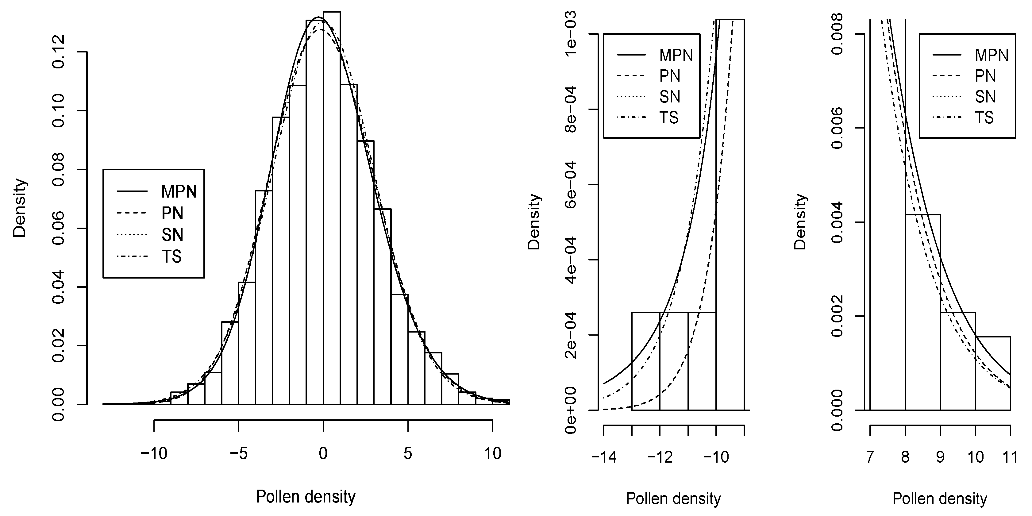
In this section, a numerical illustration based on a real dataset is presented. The goal of this application is to show empirical evidence that the yields a better fit to data than the , , and t-student with degrees of freedom distributions. For that reason, we consider a set of 3848 observations of the variable “density” included in the dataset verb “POLLEN5.DA” available at http://lib.stat.cmu.edu/datasets/pollen.data. This variable measures a geometric characteristic of a specific type of pollen. This dataset was previously used by Pewsey et al. [9] to compare the and distributions. A summary of some descriptive statistics are displayed in Table 4 below.
By using the results derived in Proposition 4, we have computed the moment estimates for the parameters of the distribution, obtaining . Then, by taking these numbers as initial values, the ML estimates are derived. In Table 5, the ML estimates for the parameters of the , , , and distributions. The figures between brackets are the asymptotic standard errors of the estimates obtained by inverting the Fisher’s information matrices for the three models evaluated at their respective ML estimates. Additionally, for each model, the values of the maximum of the log-likelihood function () are reported. The distribution attains the largest value, and consequently provides a better fit to data.
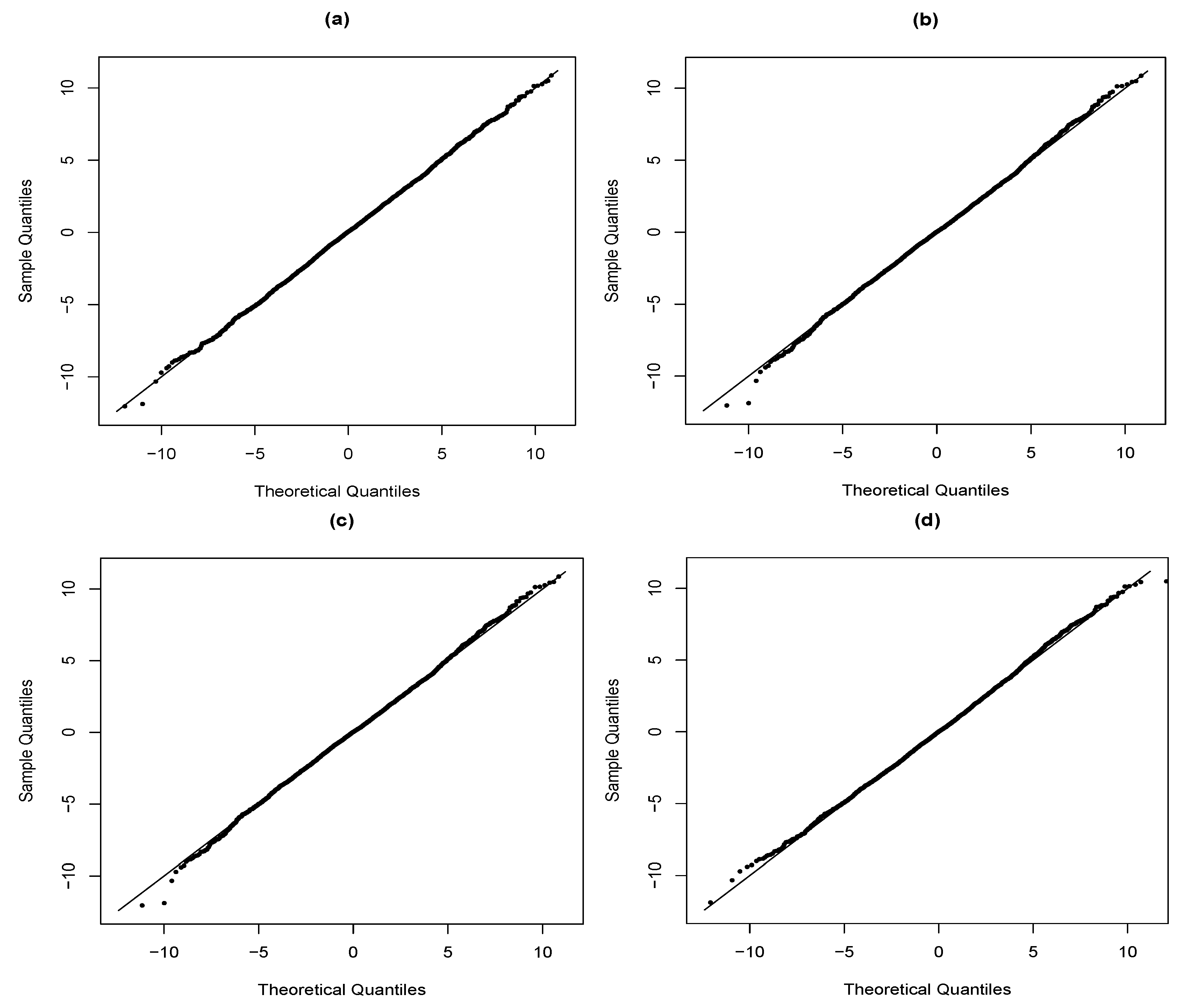
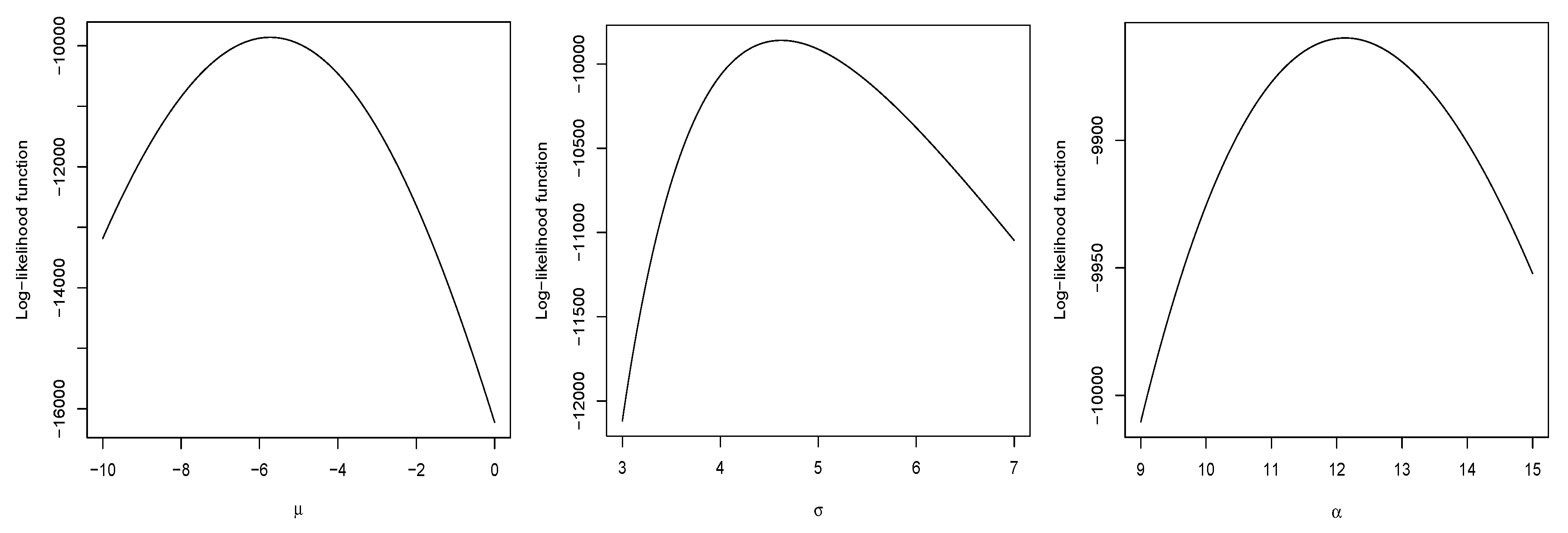
To compare the fit achieved by each distribution, the values of several measures of model selection, i.e., Akaike’s information criterion (AIC) (see Akaike [22]) and Bayesian information criterion (BIC) (see Schwarz [23]) are reported in Table 6. A model with lower numbers in these measures of model selection is preferable. It can be seen that the is preferable in terms of these two measures of model validation. In addition, the Kolmogorov–Smirnov test statistics and the corresponding p-values has been included in this table for all the models considered. It can be observed that none of the models is rejected at the usual significance levels. However, the distribution has a higher p-value and is rejected later than the other two models. Alternative methods of model selection to the Kolmogorov–Smirnov test that can be applied here can be found in Jntschi and Bolboac [24] and Jntschi [25]. Furthermore, the histogram associated to the empirical distribution of the variable “density” in the pollen dataset is illustrated in the left hand side of Figure 5. In addition, the densities of , , , and , by using the maximum likelihood estimates of their parameters, have been superimposed. Similarly, on the right hand side of Figure 5, the fit in both tails is shown. It is observable that, for this dataset, the has thicker tails than the other three distributions. Finally, the QQ-plots for each distribution considered have been illustrated in Figure 6. Here, note that the distribution exhibits an almost perfect alignment with the 45 line, and therefore it provides a better fit for extreme quantiles. Finally, Figure 7 displays the profile log-likelihood of , , and of the MPN distribution. It is noticeable that the estimates are unique.
5. Concluding Remarks
In this paper, a modification of the continuous symmetric-power distribution has been introduced. The particular case of the normal distribution the distribution has been examined in detail. This distribution arises by modifying the distribution function of the symmetrical powers family. After carrying out this modification, a more flexible family of probability distributions is obtained, allowing for the kurtosis coefficient to take a certain range of values in the parameter space. For this model, its basic properties, different method of estimation and Fisher’s information matrix were studied. By using a real dataset, we showed that the distribution provides a better fit than other existing models in the literature such as the , , and distributions.
Author Contributions
The authors contributed equally to this work.
Funding
This work was partially completed while Héctor W. Gómez visited the Universidad de Las Palmas de Gran Canaria, supported by MINEDUC-UA project, code ANT1855. This research was also funded by (EGD) [Ministerio de Economía y Competitividad, Spain] grant number [ECO2013–47092]; (EGD)[Ministerio de Economía, Industria y Competitividad. Agencia Estatal de Investigación] grant number [ECO2017–85577–P].
Acknowledgments
We also acknowledge the referee’s suggestions that helped us to improve this work.
Conflicts of Interest
The authors declare no conflicts of interest.
Appendix A
The first derivatives of are given by
The second derivatives of are
References
- Azzalini, A. A class of distributions which includes the normal ones. Scand. J. Stat. 1985, 12, 171–178. [Google Scholar]
- Arellano-Valle, R.B.; Gómez, H.W.; Quintana, F.A. A New Class of Skew-Normal Distributions. Commun. Stat. Theory Methods 2004, 33, 1465–1480. [Google Scholar] [CrossRef]
- Arellano-Valle, R.B.; Gómez, H.W.; Salinas, H.S. A note on the Fisher information matrix for the skew-generalized-normal model. Stat. Oper. Res. Trans. 2013, 37, 19–28. [Google Scholar]
- Azzalini, A. The Skew-Normal and Related Families; IMS monographs; Cambridge University Press: New York, NY, USA, 2014. [Google Scholar]
- Martínez-Flórez, G.; Barranco-Chamorro, I.; Bolfarine, H.; Gómez, H.W. Flexible Birnbaum–Saunders Distribution. Symmetry 2019, 11, 1305. [Google Scholar] [CrossRef]
- Contreras-Reyes, J.E.; Arellano-Valle, R.B. Kullback–Leibler Divergence Measure for Multivariate Skew-Normal Distributions. Entropy 2012, 14, 1606–1626. [Google Scholar] [CrossRef]
- Chiogna, M. A note on the asymptotic distribution of the maximum likelihood estimator for the scalar skew-normal distribution. Stat. Methods Appl. 2005, 14, 331–341. [Google Scholar] [CrossRef]
- Arellano-Valle, R.B.; Azzalini, A. The centred parametrization for the multivariate skew-normal distribution. J. Multivar. Anal. 2008, 99, 1362–1382. [Google Scholar] [CrossRef]
- Pewsey, A.; Gómez, H.W.; Bolfarine, H. Likelihood-based inference for power distributions. Test 2012, 21, 775–789. [Google Scholar] [CrossRef]
- Lehmann, E.L. The power of rank tests. Ann. Math. Statist. 1953, 24, 23–43. [Google Scholar] [CrossRef]
- Durrans, S.R. Distributions of fractional order statistics in hydrology. Water Resour. Res. 1992, 28, 1649–1655. [Google Scholar] [CrossRef]
- Gupta, D.; Gupta, R.C. Analyzing skewed data by power normal model. Test 2008, 17, 197–210. [Google Scholar] [CrossRef]
- Martínez-Flórez, G.; Arnold, B.C.; Bolfarine, H.; Gómez, H.W. The Multivariate Alpha-power Model. J. Stat. Plan. Inference 2013, 143, 1236–1247. [Google Scholar] [CrossRef]
- Martínez-Flórez, G.; Bolfarine, H.; Gómez, H.W. Asymmetric regression models with limited responses with an application to antibody response to vaccine. Biom. J. 2013, 55, 156–172. [Google Scholar] [CrossRef] [PubMed]
- Martínez-Flórez, G.; Bolfarine, H.; Gómez, H.W. The log alpha-power asymmetric distribution with application to air pollution. Environmetrics 2014, 25, 44–56. [Google Scholar] [CrossRef]
- Martínez-Flórez, G.; Bolfarine, H.; Gómez, H.W. Doubly censored power-normal regression models with inflation. Test 2015, 24, 265–286. [Google Scholar] [CrossRef]
- Castillo, N.O.; Gallardo, D.I.; Bolfarine, H.; Gómez, H.W. Truncated Power-Normal Distribution with Application to Non-Negative Measurements. Entropy 2018, 20, 433. [Google Scholar] [CrossRef]
- Maciak, M.; Peštová, B.; Pešta, M. Structural breaks in dependent, heteroscedastic, and extremal panel data. Kybernetika 2018, 54, 1106–1121. [Google Scholar] [CrossRef]
- Pesˇta, M. Total least squares and bootstrapping with application in calibration. Statistics 2013, 47, 966–991. [Google Scholar] [CrossRef]
- Shaked, M.; Shanthikumar, J.G. Stochastic Orders; Springer Science & Business Media: New York, NY, USA, 2007. [Google Scholar]
- R Development Core Team. A Language and Environment for Statistical Computing; R Foundation for Statistical Computing: Vienna, Austria, 2019. [Google Scholar]
- Akaike, H. A new look at the statistical model identification. IEEE Trans. Autom. Control 1974, 19, 716–723. [Google Scholar] [CrossRef]
- Schwarz, G. Estimating the dimension of a model. Ann. Statist. 1978, 6, 461–464. [Google Scholar] [CrossRef]
- Ja¨ntschi, L.; Bolboacă, S.D. Computation of Probability Associated with Anderson–Darling Statistic. Mathematics 2018, 6, 88. [Google Scholar] [CrossRef]
- Ja¨ntschi, L. A Test Detecting the Outliers for Continuous Distributions Based on the Cumulative Distribution Function of the Data Being Tested. Symmetry 2019, 11, 835. [Google Scholar] [CrossRef] [Green Version]
Figure 1.
Plot of the pdf of distribution for selected values of the parameters.

Figure 2.
Plot of the first derivative of distribution for selected values of the parameters.

Figure 3.
Plot of the and of the distribution.

Figure 4.
Graphs of the skewness and kurtosis coefficients for the and distributions.

Figure 5.
Left panel: Histogram of the empirical distribution and fitted densities by ML superimposed for pollen dataset. Right panel: Plots of the tails for the four models.
Figure 5.
Left panel: Histogram of the empirical distribution and fitted densities by ML superimposed for pollen dataset. Right panel: Plots of the tails for the four models.

Figure 6.
QQ-plots: (a) model; (b) model; (c) model; (d) model.

Figure 7.
Profile log-likelihood of , and for the distribution.


Table 1.
Approximations of the roots of Equations (9) and (10) for some values of , and the corresponding figures of the pdf of the evaluated at these roots.
| 0.5 | −0.136 | −1.135 | 0.886 | 0.397 | 0.239 | 0.241 |
| 1.0 | 0.000 | −1.000 | 1.000 | 0.399 | 0.242 | 0.242 |
| 2.0 | 0.243 | −0.691 | 1.173 | 0.412 | 0.261 | 0.251 |
| 3.0 | 0.435 | −0.414 | 1.299 | 0.433 | 0.282 | 0.266 |
| 4.0 | 0.586 | −0.203 | 1.396 | 0.457 | 0.298 | 0.284 |
| 5.0 | 0.706 | −0.041 | 1.475 | 0.481 | 0.316 | 0.301 |
Table 2.
Approximations of and of the distribution for different values of .
| 0.5 | −0.097 | 1.006 |
| 1.0 | 0.000 | 1.000 |
| 5.0 | 0.659 | 0.770 |
| 10.0 | 1.119 | 0.521 |
| 100.0 | 2.247 | 0.218 |
Table 3.
Maximum likelihood (ML) estimates and standard deviation (SD) for the parameters , and of the model for different generated samples of sizes 100, and 200.
Table 3.
Maximum likelihood (ML) estimates and standard deviation (SD) for the parameters , and of the model for different generated samples of sizes 100, and 200.
| (SD) | (SD) | (SD) | |||
| 0 | 1 | 0.1 | −0.352478 (0.149214) | 0.994441 (0.091321) | 0.190243 (0.175202) |
| 0.5 | −0.19534 (0.14501) | 0.990622 (0.094550) | 0.613052 (0.272096) | ||
| 0.8 | −0.083183 (0.144587) | 0.990286 (0.098669) | 0.854338 (0.164924) | ||
| 1 | −0.009586 (0.141691) | 0.995312 (0.0997256) | 1.007328 (0.122688) | ||
| 5 | 0.004225 (0.100001) | 0.997408 (0.088254) | 5.030272 (0.229064) | ||
| 10 | 0.001108 (0.066610) | 0.999124 (0.068611) | 10.060478 (0.475019) | ||
| 100 | 0.002171 (0.017362) | 1.001152 (0.029604) | 100.437990 (2.668190) | ||
| 0 | 1 | 0.1 | −0.351446 (0.104552) | 0.998513 (0.070831) | 0.180054 (0.111930) |
| 0.5 | −0.19268 (0.101786) | 0.997622 (0.068806) | 0.576957 (0.223378) | ||
| 0.8 | −0.08140 (0.099360) | 0.997674 (0.069451) | 0.830318 (0.152995) | ||
| 1 | 0.002786 (0.097411) | 0.996444 (0.069648) | 1.002200 (0.088749) | ||
| 5 | 0.002014 (0.099305) | 0.996788 (0.085987) | 5.023032 (0.221756) | ||
| 10 | 0.002897 (0.046109) | 1.000515 (0.050192) | 10.032857 (0.339106) | ||
| 100 | 0.000623 (0.012137) | 1.000185 (0.019759) | 100.168752 (1.866302) | ||
| 0 | 1 | 0.1 | −0.348177 (0.072732) | 0.999433 (0.047548) | 0.170978 (0.076165) |
| 0.5 | −0.196617 (0.072015) | 0.999142 (0.047896) | 0.562935 (0.218890) | ||
| 0.8 | −0.076657 (0.069510) | 0.997719 (0.050718) | 0.824700 (0.127661) | ||
| 1 | 0.001158 (0.06877) | 0.998408 (0.050586) | 1.003651 (0.058344) | ||
| 5 | −0.000165 (0.053006) | 1.000623 (0.044182) | 5.005130 (0.115719) | ||
| 10 | −0.000239 (0.033615) | 1.000017 (0.035902) | 10.014958 (0.246652) | ||
| 100 | 0.000514 (0.008452) | 1.000491 (0.014599) | 100.104380 (1.295144) | ||
Table 4.
Summary of descriptive statistics for the pollen density dataset.
| Mean | Median | Variance | Skewness | Kurtosis |
|---|---|---|---|---|
| 0.000 | −0.030 | 9.887 | 0.109 | 3.193 |
Table 5.
Parameter estimates; standard errors (SE); and maximum of the log-likelihood function, , for the , , , and corresponding to the pollen density dataset.
Table 5.
Parameter estimates; standard errors (SE); and maximum of the log-likelihood function, , for the , , , and corresponding to the pollen density dataset.
| Parameters | ||||
|---|---|---|---|---|
| −0.010 (0.05) | −2.04 (0.24) | −1.74 (0.68) | −5.73 (0.43) | |
| 3.037 (0.05) | 3.75 (0.14) | 3.69 (0.21) | 4.62 (0.14) | |
| 29.995 (13.01) | 0.93 (0.14) | 1.77 (0.37) | 12.13 (1.21) | |
| −9864.99 | −9863.42 | −9863.37 | −9861.98 |
Table 6.
Akaike’s information criterion (AIC), Bayesian information criterion (BIC), Kolmogorov– Smirnov (KSS) test, and the corresponding p-values for all the models considered.
Table 6.
Akaike’s information criterion (AIC), Bayesian information criterion (BIC), Kolmogorov– Smirnov (KSS) test, and the corresponding p-values for all the models considered.
| Criteria | ||||
|---|---|---|---|---|
| AIC | 19,735.98 | 19,732.84 | 19,732.74 | 19,729.96 |
| BIC | 19,754.74 | 19,751.61 | 19,751.50 | 19,748.72 |
| KSS (p-value) | 0.014 (0.516) | 0.013 (0.559) | 0.012 (0.627) | 0.010 (0.820) |
© 2019 by the authors. Licensee MDPI, Basel, Switzerland. This article is an open access article distributed under the terms and conditions of the Creative Commons Attribution (CC BY) license (http://creativecommons.org/licenses/by/4.0/).
Share and Cite
MDPI and ACS Style
Gómez-Déniz, E.; Iriarte, Y.A.; Calderín-Ojeda, E.; Gómez, H.W. Modified Power-Symmetric Distribution. Symmetry 2019, 11, 1410. https://0-doi-org.brum.beds.ac.uk/10.3390/sym11111410
AMA Style
Gómez-Déniz E, Iriarte YA, Calderín-Ojeda E, Gómez HW. Modified Power-Symmetric Distribution. Symmetry. 2019; 11(11):1410. https://0-doi-org.brum.beds.ac.uk/10.3390/sym11111410
Chicago/Turabian StyleGómez-Déniz, Emilio, Yuri A. Iriarte, Enrique Calderín-Ojeda, and Héctor W. Gómez. 2019. "Modified Power-Symmetric Distribution" Symmetry 11, no. 11: 1410. https://0-doi-org.brum.beds.ac.uk/10.3390/sym11111410
Note that from the first issue of 2016, this journal uses article numbers instead of page numbers. See further details here.