The Grimus–Neufeld Model with FlexibleSUSY at One-Loop
by
 , , ,
, , ,
Simonas Draukšas
 ,
,
Vytautas Dūdėnas
,
Thomas Gajdosik
*,
Andrius Juodagalvis
,
Paulius Juodsnukis
and
Darius Jurčiukonis
Institute of Theoretical Physics and Astronomy, Faculty of Physics, Vilnius University, Saulėtekio av. 3, 10257 Vilnius, Lithuania
*
Author to whom correspondence should be addressed.
Symmetry 2019, 11(11), 1418; https://0-doi-org.brum.beds.ac.uk/10.3390/sym11111418
Submission received: 28 October 2019
/
Revised: 11 November 2019
/
Accepted: 12 November 2019
/
Published: 16 November 2019
(This article belongs to the Special Issue Selected Papers from 43rd International Conference of Theoretical Physics: Matter to the Deepest, Recent Developments In Physics Of Fundamental Interactions (MTTD2019))
Abstract
:The Grimus–Neufeld model can explain the smallness of measured neutrino masses by extending the Standard Model with a single heavy neutrino and a second Higgs doublet, using the seesaw mechanism and radiative mass generation. The Grimus–Lavoura approximation allows us to calculate the light neutrino masses analytically. By inverting these analytic expressions, we determine the neutrino Yukawa couplings from the measured neutrino mass differences and the neutrino mixing matrix. Short-cutting the full renormalization of the model, we implement the Grimus–Neufeld model in the spectrum calculator FlexibleSUSY and check the consistency of the implementation. These checks hint that FlexibleSUSY is able to do the job of numerical renormalization in a restricted parameter space. As a summary, we also comment on further steps of the implementation and the use of FlexibleSUSY for the model.
PACS:
11.30.Rd; 13.15.+g; 14.60.St1. Introduction
The last 30 years of collider physics showed an ever-increasing success for the predictions of the Standard Model (SM) [1]. A similar statement can be said about the experimental program in neutrino physics [2], but no unambiguous common treatment for both areas exists up to now. The masses and the mixing of neutrinos can easily be formulated in a Lagrangian picture; nevertheless, these terms in the Lagrangian are still considered to be “beyond the Standard Model” (BSM). Whereas the formulation of the SM and the accurate calculations for the experimental predictions require the framework of Quantum Feld Theory (QFT), the analysis of neutrino measurements is still done in the framework of plain Quantum Mechanics (QM); an explanation of why QM is usually enough for the study of neutrino oscillations can be found in [3].
The usual two explanations of the smallness of neutrino masses in the Lagrangian context are the seesaw mechanism [4] or radiative mass generation for the light neutrinos [5,6,7,8]. In 1989, Walter Grimus and Helmut Neufeld pointed to the possibility that both mechanisms can be comparable for explaining the masses of the light neutrinos [9]. We call the minimal extension of the SM that allows this feature Grimus–Neufeld Model (GNM). This minimal extension adds to the SM only a single heavier Majorana singlet and one additional Higgs doublet. The qualitative behavior of the GNM is described in [10]. An extended description of our approach is presented in [11]. Here, we review shortly the features of the GNM and discuss its implementation in FlexibleSUSY [12,13], which uses SARAH [14,15,16,17] and SOFTSUSY [18,19]. This implementation gives us a tool to check the renormalization and the consistency of the model numerically.
The main aim of this work is to discuss the plans for the checks of the model and the possible modifications that can be done to the code. The first trials of the implemented code hint that, to have only small loop corrections, the model has a natural preference for a small seesaw scale.
2. Results
2.1. Summary of Features of the Grimus–Neufeld Model
2.1.1. Lagrangian
Since the GNM is a minimal extension of the SM, we only need to give the additional parts of the Lagrangian. These are the Majorana mass term for the fermionic singlet N
the Yukawa terms (ignoring quarks) among the lepton doublets , the Higgs doublets , and either the charged lepton singlets or the fermionic singlet N
and the Higgs potential
which is just the generic two Higgs doublet potential, which we write in the Higgs basis [20], meaning that only has a vacuum expectation value (vev) v. in Equation (1) is the Lorentz covariant conjugate [21] of , which is the right-chiral part of N.
2.1.2. Tree-Level Mass Matrices and Tree-Level Masses
As we are interested mainly in the neutrino sector, we deal only with the mass matrices of the leptons and the Higgs bosons. For the charged leptons, the relevant Yukawa coupling is , since we work in the Higgs basis. Then, diagonalization of the charged lepton mass matrix ,
defines the mass eigenstates for the charged leptons and, consequently, the flavor basis for the SM neutrino fields , which are the partners of the charged leptons in the weak lepton doublets.
The mass matrix for the neutrinos in the GNM in flavor basis at tree level is the symmetric -matrix ,
which is only rank 2 and therefore has only two non-vanishing singular values. That means we have the heavy mass and only a single light, massive neutrino with mass coming from the seesaw. The two other masses are zero at tree level. The radiative mass will be at one-loop, but the remaining other neutrino with mass stays massless even at one-loop level.
Following the idea in [22,23] to formulate the 2HDM potential in terms of basis independent physical quantities, we skip the discussion of the mass matrix of the Higgs bosons and point the reader to the relevant literature [20,24,25,26]. For the tree-level masses of the Higgs bosons, we just want to note that we take the lightest boson, h, to correspond to the boson observed at the LHC with the mass GeV [1]. The other Higgs boson masses are free parameters subject to the experimental constraints.
2.1.3. Leading Order Loop-Level Masses
The observation that the predicted loop-level mass for one neutrino, , can be of the same order as the seesaw generated mass was the main point of the paper of Grimus and Neufeld [9] in 1989. Since the remaining neutrino stays massless at one-loop order, , and all other particles already have a mass (unless they are protected by an unbroken gauge symmetry), this radiative neutrino mass is the main effect at one loop. This predicted mass is finite and gauge invariant, as proven in [10,27,28] using different approaches. One loop radiative corrections affect the seesaw generated neutrino mass , too. We denote the resulting mass as .
2.2. The Grimus–Lavoura Approximation
The full calculation of the renormalized neutrino masses for the GNM in analytic form is not available yet. We adapt the proof of finiteness and gauge invariance of the one-loop corrections to the effective light neutrino mass matrix from [27] and formulate the Grimus–Lavoura approximation for calculating light neutrino masses:
- Staying in the interaction eigenstates, as defined by the charged leptons, calculate the neutrino mass matrix using Equation (5).
- Reducing the problem to the light neutrinos, one arrives at the effective symmetric neutrino mass matrix , which has the tree-level valuethat has obviously rank 1 and will give only the neutrino mass . However, at one-loop, this matrix becomeswithWith this correction, can have rank .
- The approximation consists now of:
- Assuming to be irrelevant for the light neutrinos with the reasoning that (or ) is not measured. It is still a free parameter of the theory that can be adjusted as needed.
- Observing that the corrections with are subdominant, because they are suppressed by the squares of small Yukawa or gauge couplings and additionally by the small charged lepton masses.
- Assuming that the loop correction is of the same order as the tree-level value .
The result of this approximation is that we can derive analytic formulas that predict the masses of the light neutrinos, as depending on the tree-level input parameters:
where . are the basis-independent mixing angles of the neutral Higgs fields [20]. Following Grzadkowski et al. [22], these angles can be expressed by the -couplings as
2.3. Using the Grimus–Lavoura Approximation
Since our model predicts one neutrino mass to remain zero at one-loop level (), we can use the measured neutrino mass squared differences [2] to determine the values of the other light neutrino masses .
Parameterizing the neutrino Yukawa couplings as
with three orthonormal three-vectors , we can invert the analytic expressions of the masses, Equation (9), and determine the parameters d and . The explicit formulas and the discussion of the difficulties in finding solutions for can be found in [11]. The values of d and do not depend on the three orthonormal three-vectors . At tree-level, these vectors can be understood as an approximate neutrino mixing matrix , as it diagonalizes the effective tree-level neutrino mass matrix with the Takagi decomposition:
Applying these same vectors to the effective one-loop neutrino mass matrix
we see that the effective one-loop neutrino mass matrix is rank 2, and hence provides two massive light neutrino states. The full neutrino mixing matrix should diagonalize the full one-loop mass matrix
A reordering of the masses is possible, if . For a more detailed discussion, see [11].
As a side note: The minus-sign on the right-hand side of Equation (12) comes from the convention of the seesaw, where the seesaw rotation is written with an orthogonal matrix and the minus sign kept to be absorbed in the phase of the light state. We do not write a minus-sign on the right-hand side of Equation (14) following the convention of the normal singular value decomposition and the positivity of the masses. The phase in this second case is part of the complex mixing matrix.
2.4. The One-Loop Improved Lagrangian
Using the neutrino Yukawa couplings as defined in the previous subsection, the determination of the Higgs potential parameters following Grzadkowski et al. [22], and the identification of the singlet mass parameter with the heavy neutrino mass , we get a new parametrization of the Lagrangian as
the Yukawa terms
where d and are functions depending on the same parameters as , Equation (15), and the Higgs potential
is expressed in terms of physical masses and couplings of the Higgs bosons.
As an advantage, more parameters of the one-loop improved Lagrangian correspond directly to measured quantities: instead of six complex parameters in two-neutrino Yukawa couplings in , contains two real selectable parameters ( and ), two real parameters that we determine from the measured neutrino mass squared differences (d and ), and six parameters in the vectors that we determine from the measured neutrino mixing matrix . One of the two “missing” parameters in is the vanishing one-loop level neutrino mass, and the other parameter is the undeterminable Majorana phase of this zero-mass neutrino.
2.5. Renormalizing the GNM
The final goal of our efforts is to fully renormalize the GNM. The full renormalization will also indicate the importance and validity of the one-loop improved Lagrangian. However, we are still far from that goal. Only the mass renormalization of light neutrinos has been tackled in detail [28,29]. Since the full renormalization is difficult, we plan to use a spectrum calculator that performs the renormalization numerically. A foreseeable difficulty lies in the hierarchy of the seesaw. It is hard to have a reliable numerical implementation of the mass hierarchies of more than 10 orders of magnitude. We found that FlexibleSUSY [13] is able to do the job if we limit the seesaw scale. Now, we can study the renormalized model, but only numerically.
2.6. FlexibleSUSY for the GNM in a Nutshell
The primary idea of FlexibleSUSY was to numerically implement the renormalization group running of a model between two scales and to be able to give boundary conditions on both scales. In the case of a SUSY-GUT, one can require the low energy measured masses and couplings as one boundary condition and the GUT constraints at the GUT scale as another boundary condition. Then, the program tries to find a numerical solution that interpolates between the two scales and fulfills both boundary conditions.
In our case, we do not have the high scale, and we are not interested in imposing conditions at a scale other than our low scale. However, with the accuracy needed for today’s collider physics, one has to interpolate between the various scales of the different measurements that determine the masses and couplings of the SM and also the masses and mixing parameters of the neutrino sector. That means that the capabilities of FlexibleSUSY are needed also for implementing models that “live” only at the low scale.
To implement a model in FlexibleSUSY, one has first to define the Lagrangian of the model with SARAH [14,15,16,17] and check the consistency and completeness of the Lagrangian. In the next step, FlexibleSUSY uses SARAH to produce the model code. Additionally, one has to define the boundary conditions in a separate steering file, using the convention for the names of fields implemented in SARAH. This step includes the definition of what is to be treated as input and what is the desired output for the spectrum to be calculated. When this is done, one has to compile the generated code to get the actual spectrum calculator for the implemented model.
This program can be used from the terminal with the help of input and output files in the SLHA [30,31] format. That means writing the values of the input parameters and additional optional arguments into the SLHA input file and the program writes from this input the SLHA output file, which contains the mass spectrum of the model and also the decay rates of the particles of the model.
Another option to use the program is from the provided Mathematica™ [32] interface. There, the playing around with parameters and the generation of plots become much easier, but the comparison of results with other scientists becomes less accurate or much more cumbersome.
2.6.1. Our Achievements with the GNM in FlexibleSUSY
We succeeded to implement the basic Lagrangian of the GNM, in Equations (1)–(3), in FlexibleSUSY and to generate a working code. This code could qualitatively reproduce the effect of the seesaw mechanism. However, it was difficult to find a point in the Higgs potential that gives sensible results for the Higgs masses also at one-loop level. This might be due to our limited experience with spectrum calculators and numerics. However, we are learning a lot of physics while trying to figure out where the problems can come from.
2.6.2. Plans with the GNM in FlexibleSUSY
The first step is to check our implementation:
- Do we understand the tree-level correctly?
- Are the different formulations of defining the input parameters really equivalent?
- Does the GL approximation give correct neutrino masses not only at leading order, but also at full one-loop level?
- Is the limitation of the seesaw scale a numeric artifact from the finite precision or can we find a physical reason for the limitation?
The next step is to investigate the parameter space of the GNM at one-loop level, i.e., going beyond the analysis of Jurčiukonis et al. [11]. The real restrictions to the model come from comparing to measurements. We hope to recycle the FlexibleSUSY implementations of predictions of other models that are already implemented in FlexibleSUSY. One definite goal is to work out the connection between the low-energy observables such as , , and , which is caused by the GNM. Another goal for the future is to work out the implications of the GNM for cosmology, where the question might be, if the heavy singlet can be a candidate for the dark matter.
3. Discussion
The main result is the implementation and the analytic check of the Grimus–Lavoura approximation in the Grimus–Neufeld model (GNM) to replace the Yukawa couplings with the measured masses and oscillation parameters as the input for the model. The model itself [9] and the approximation [33] do not try to estimate the model parameters from measurements. In addition, the renormalization group analysis of this model in the limit of heavy right-handed neutrinos and heavy Higgs doublets [10] does not provide the explicit analytical and numerical analysis that is given in [11] and is shortly recapitulated in this paper.
The additional content of this presentation compared to the one in [11] is to address the question of the full renormalization of the GNM. The first steps in that direction were done in [29], but the full and explicit formulation of the renormalization of the GNM is work in progress with its end still far away.
To shorten the time to some results, we propose the use of generic spectrum calculators and give an account on the progress achieved with FlexibleSUSY, which is such a spectrum calculator. The final goal from both approaches, of the analytic one with fully renormalizing the model and of the numeric one with FlexibleSUSY, is to test the GNM with measurements. To that end, we want to give predictions that can be tested, such as correlations of low energy observables or correlations between the decay rates of heavy particles, which are influenced by the neutrino Yukawa coupling.
Author Contributions
Conceptualization: T.G.; methodology: T.G., S.D. and V.D.; software: S.D. and P.J.; validation: T.G., V.D. and D.J.; formal analysis: D.J.; investigation: S.D., V.D., P.J. and D.J.; data curation: D.J.; writing—original draft preparation: T.G.; writing—review and editing: T.G., S.D., V.D., A.J., P.J. and D.J.; visualization: T.G.; supervision: T.G. and A.J.; project administration: T.G. and A.J.; and funding acquisition: A.J.
Funding
This research was funded by the Lithuanian Academy of Sciences.
Acknowledgments
The authors are thankful for the very helpful discussions with Dominik Stöckinger and Wojciech Kotlarski at the conference “Matter to the Deepest 2019”.
Conflicts of Interest
The authors declare no conflict of interest.
Abbreviations
The following abbreviations are used in this manuscript:
| 2HDM | two Higgs doublet model |
| BSM | beyond the standard model physics |
| GNM | Grimus–Neufeld model |
| GUT | grand unified theory |
| LHC | large hadron collider |
| PMNS | Pontecorvo–Maki–Nakagawa–Sakata matrix |
| QFT | quantum field theory |
| QM | quantum mechanics |
| SM | standard model |
References
- Tanabashi, M.; Hagiwara, K.; Hikasa, K.; Nakamura, K.; Sumino, Y.; Takahashi, F.; Tanaka, J.; Agashe, K.; Aielli, G.; Amsler, C.; et al. Review of Particle Physics. Phys. Rev. D 2018, 98, 030001. [Google Scholar] [CrossRef]
- De Salas, P.F.; Forero, D.V.; Ternes, C.A.; Tortola, M.; Valle, J.W.F. Status of neutrino oscillations 2018: 3σ hint for normal mass ordering and improved CP sensitivity. Phys. Lett. B 2018, 782, 633–640. [Google Scholar] [CrossRef]
- Akhmedov, E.K.; Kopp, J. Neutrino Oscillations: Quantum Mechanics vs. Quantum Field Theory. J. High Energy Phys. 2010. [Google Scholar] [CrossRef]
- Schechter, J.; Valle, J. Neutrino Masses in SU(2) × U(1) Theories. Phys. Rev. D 1980, 22, 2227. [Google Scholar] [CrossRef]
- Zee, A. A Theory of Lepton Number Violation, Neutrino Majorana Mass, and Oscillation. Phys. Lett. B 1980, 93, 389. [Google Scholar] [CrossRef]
- Branco, G.C.; Geng, C.Q. Naturally Small Dirac Neutrino Masses in Superstring Theories. Phys. Rev. Lett. 1987, 58, 969. [Google Scholar] [CrossRef]
- Chang, D.; Mohapatra, R.N. Small and Calculable Dirac Neutrino Mass. Phys. Rev. Lett. 1987, 58, 1600. [Google Scholar] [CrossRef]
- Babu, K.S. Model of ‘Calculable’ Majorana Neutrino Masses. Phys. Lett. B 1988, 203, 132–136. [Google Scholar] [CrossRef]
- Grimus, W.; Neufeld, H. Radiative Neutrino Masses in an SU(2) × U(1) Model. Nucl. Phys. B 1989, 325, 18. [Google Scholar] [CrossRef]
- Ibarra, A.; Simonetto, C. Understanding neutrino properties from decoupling right-handed neutrinos and extra Higgs doublets. J. High Energy Phys. 2011, 11, 022. [Google Scholar] [CrossRef]
- Jurčiukonis, D.; Gajdosik, T.; Juodagalvis, A. Seesaw neutrinos with one right-handed singlet field and a second Higgs doublet. arXiv 2019, arXiv:hep-ph/1909.00752. [Google Scholar]
- Athron, P.; Park, J.H.; Stöckinger, D.; Voigt, A. FlexibleSUSY—A spectrum generator generator for supersymmetric models. Comput. Phys. Commun. 2015, 190, 139–172. [Google Scholar] [CrossRef]
- Athron, P.; Bach, M.; Harries, D.; Kwasnitza, T.; Park, J.H.; Stöckinger, D.; Voigt, A.; Ziebell, J. FlexibleSUSY 2.0: Extensions to investigate the phenomenology of SUSY and non-SUSY models. arXiv 2017, arXiv:hep-ph/1710.03760. [Google Scholar] [CrossRef]
- Staub, F. From Superpotential to Model Files for FeynArts and CalcHep/CompHep. Comput. Phys. Commun. 2010, 181, 1077–1086. [Google Scholar] [CrossRef]
- Staub, F. Automatic Calculation of supersymmetric Renormalization Group Equations and Self Energies. Comput. Phys. Commun. 2011, 182, 808–833. [Google Scholar] [CrossRef]
- Staub, F. SARAH 3.2: Dirac Gauginos, UFO output, and more. Comput. Phys. Commun. 2013, 184, 1792–1809. [Google Scholar] [CrossRef]
- Staub, F. SARAH 4: A tool for (not only SUSY) model builders. Comput. Phys. Commun. 2014, 185, 1773–1790. [Google Scholar] [CrossRef]
- Allanach, B. SOFTSUSY: A program for calculating supersymmetric spectra. Comput. Phys. Commun. 2002, 143, 305–331. [Google Scholar] [CrossRef]
- Allanach, B.; Athron, P.; Tunstall, L.C.; Voigt, A.; Williams, A. Next-to-Minimal SOFTSUSY. Comput. Phys. Commun. 2014, 185, 2322–2339. [Google Scholar] [CrossRef]
- Haber, H.E.; O’Neil, D. Basis-independent methods for the two-Higgs-doublet model. II. The Significance of tan beta. Phys. Rev. D 2006, 74, 015018. [Google Scholar] [CrossRef]
- Pal, P.B. Dirac, Majorana and Weyl fermions. Am. J. Phys. 2011, 79, 485–498. [Google Scholar] [CrossRef]
- Grzadkowski, B.; Haber, H.E.; Ogreid, O.M.; Osland, P. Heavy Higgs boson decays in the alignment limit of the 2HDM. J. High Energy Phys. 2018, 12, 056. [Google Scholar] [CrossRef]
- Grzadkowski, B.; Ogreid, O.M.; Osland, P. The CP-symmetries of the 2HDM. In Proceedings of the 6th Symposium on Prospects in the Physics of Discrete Symmetries (DISCRETE 2018), Vienna, Austria, 26–30 November 2018. [Google Scholar]
- Davidson, S.; Haber, H.E. Basis-independent methods for the two-Higgs-doublet model. Phys. Rev. D 2005, 72, 035004. [Google Scholar] [CrossRef]
- Haber, H.E.; O’Neil, D. Basis-independent methods for the two-Higgs-doublet model III: The CP-conserving limit, custodial symmetry, and the oblique parameters S, T, U. Phys. Rev. D 2011, 83, 055017. [Google Scholar] [CrossRef]
- Branco, G.C.; Ferreira, P.M.; Lavoura, L.; Rebelo, M.N.; Sher, M.; Silva, J.P. Theory and phenomenology of two-Higgs-doublet models. Phys. Rept. 2012, 516, 1–102. [Google Scholar] [CrossRef]
- Grimus, W.; Lavoura, L. Soft lepton flavor violation in a multi Higgs doublet seesaw model. Phys. Rev. D 2002, 66, 014016. [Google Scholar] [CrossRef]
- Dūdėnas, V.; Gajdosik, T. Gauge dependence of tadpole and mass renormalization for a seesaw extended 2HDM. Phys. Rev. D 2018, 98, 035034. [Google Scholar] [CrossRef]
- Dūdėnas, V. Renormalization of Neutrino Masses in the Grimus-Neufeld Model; Vilniaus Universiteto Leidykla: Vilnius, Lithuania, 2019. [Google Scholar]
- Allanacha, B.C.; Balázs, C.; Bélanger, G.; Bernhardt, M.; Boudjema, F.; Choudhury, D.; Desch, K.; Ellwanger, U.; Gambino, P.; Godbole, R.; et al. SUSY Les Houches Accord 2. Comput. Phys. Commun. 2009, 180, 8–25. [Google Scholar] [CrossRef]
- Basso, L.; Belyaev, A.; Chowdhury, D.; Hirsch, M.; Khalil, S.; Moretti, S.; O’Leary, B.; Porod, W.; Staub, F. Proposal for generalised Supersymmetry Les Houches Accord for see-saw models and PDG numbering scheme. Comput. Phys. Commun. 2013, 184, 698–719. [Google Scholar] [CrossRef]
- Wolfram Research, Inc. Mathematica; Version 12.0; Wolfram Research, Inc.: Champaign, IL, USA, 2019. [Google Scholar]
- Grimus, W.; Lavoura, L. One loop corrections to the seesaw mechanism in the multiHiggs doublet standard model. Phys. Lett. B 2002, 546, 86–95. [Google Scholar] [CrossRef] [Green Version]
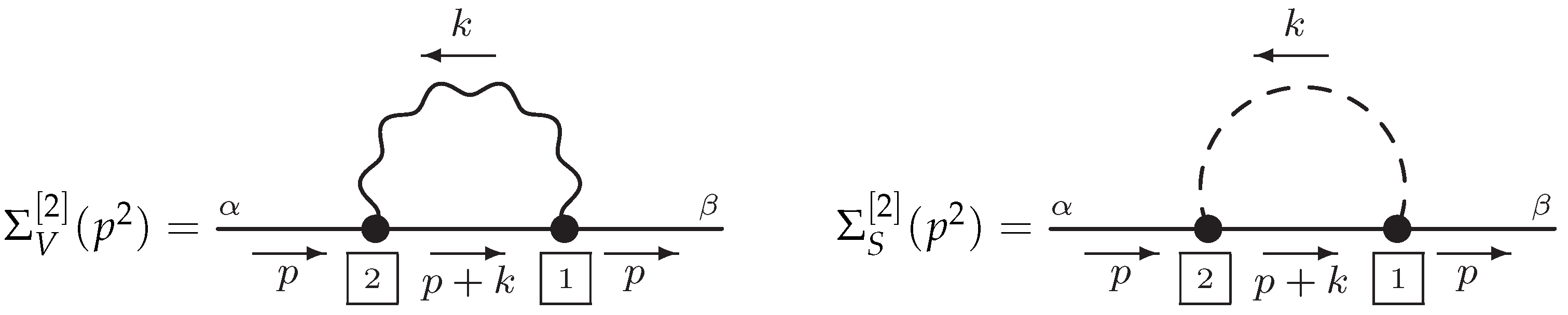
Figure 1.
Feynman diagrams contributing to the self-energies of the light neutrinos. For the correction to the mass, the internal fermion line has to be a Majorana propagator with a mass insertion; hence, charged particles will not contribute to at this loop level.
Figure 1.
Feynman diagrams contributing to the self-energies of the light neutrinos. For the correction to the mass, the internal fermion line has to be a Majorana propagator with a mass insertion; hence, charged particles will not contribute to at this loop level.

© 2019 by the authors. Licensee MDPI, Basel, Switzerland. This article is an open access article distributed under the terms and conditions of the Creative Commons Attribution (CC BY) license (http://creativecommons.org/licenses/by/4.0/).
Share and Cite
MDPI and ACS Style
Draukšas, S.; Dūdėnas, V.; Gajdosik, T.; Juodagalvis, A.; Juodsnukis, P.; Jurčiukonis, D. The Grimus–Neufeld Model with FlexibleSUSY at One-Loop. Symmetry 2019, 11, 1418. https://0-doi-org.brum.beds.ac.uk/10.3390/sym11111418
AMA Style
Draukšas S, Dūdėnas V, Gajdosik T, Juodagalvis A, Juodsnukis P, Jurčiukonis D. The Grimus–Neufeld Model with FlexibleSUSY at One-Loop. Symmetry. 2019; 11(11):1418. https://0-doi-org.brum.beds.ac.uk/10.3390/sym11111418
Chicago/Turabian StyleDraukšas, Simonas, Vytautas Dūdėnas, Thomas Gajdosik, Andrius Juodagalvis, Paulius Juodsnukis, and Darius Jurčiukonis. 2019. "The Grimus–Neufeld Model with FlexibleSUSY at One-Loop" Symmetry 11, no. 11: 1418. https://0-doi-org.brum.beds.ac.uk/10.3390/sym11111418
Note that from the first issue of 2016, this journal uses article numbers instead of page numbers. See further details here.