A Novel Method to Identify Initial Values of Chaotic Maps in Cybersecurity

1
Department of Electrical Engineering, HITEC University, Taxila 47080, Pakistan
2
Department of Mathematics, Statistics and Physics, Qatar University, Doha 2713, Qatar
*
Author to whom correspondence should be addressed.
Symmetry 2019, 11(2), 140; https://0-doi-org.brum.beds.ac.uk/10.3390/sym11020140
Submission received: 11 November 2018
/
Revised: 10 January 2019
/
Accepted: 15 January 2019
/
Published: 27 January 2019
Abstract
:Chaos theory has applications in several disciplines and is focusing on the behavior of dynamical systems that are highly sensitive to initial conditions. Chaotic dynamics are the impromptu behavior displayed by some nonlinear dynamical frameworks and have been used as a source of diffusion in cybersecurity for more than two decades. With the addition of chaos, the overall strength of communication security systems can be increased, as seen in recent proposals. However, there is a major drawback of using chaos in communication security systems. Chaotic communication security systems rely on private keys, which are the initial values and parameters of chaotic systems. This paper shows that these chaotic communication security systems can be broken by identifying those initial values through the statistical analysis of standard deviation and variance. The proposed analyses are done on the chaotic sequences of Lorenz chaotic system and Logistic chaotic map and show that the initial values and parameters, which serve as security keys, can be retrieved and broken in short computer times. Furthermore, the proposed model of identifying the initial values can also be applied on other chaotic maps as well.
1. Introduction
In physics, jerk is the third derivative of position, with respect to time. It has been shown that a jerk equation, which is equivalent to a system of three first-order, ordinary, non-linear differential equations, is in a certain sense the minimal setting for solutions showing chaotic behavior. Therefore, chaos [1,2,3,4] has many applications in physics. With the exponential increase in information technology devices, the need for reliable authentication solutions has also been increased [5,6]. The traditional passive authentication systems that require the indirect involvement of users proves to be ineffective, e.g., loss or wrongful acquisition of username and password by an unapproved client results in loss of confidential data [7]. In contrast, a biometric authentication system, which is based on physical attributes of users, can be much more effective and secure [8]. The physical attributes can be fingerprint, face recognition, palm veins, palm print, DNA, hand geometry, retina, iris recognition and odor/scent [9]. Biometrics cannot easily be stolen, lost, duplicated, hacked, or shared; additionally, they are impervious to social designing assaults since clients are obliged to be available to utilize a biometric component. In recent years, there has been a rapid increase seen in publication of new biometrics and security algorithms that use the application of nonlinear dynamics, such as chaos theory [10,11,12,13,14,15,16,17,18,19].
Chaos [20,21,22,23] is a kind of science that deals with parts of the world that are unpredictable, apparently random, not necessarily random, disorderly auratic and irregular misbehaved. A class of models is identified [24] that can represent the two-phase microfluidic flow in different experimental conditions. The identification procedure adopted is based on the nonlinear systems synchronization theory. Formally, chaos theory was introduced by a meteorologist, Edward N. Lorenz [25], who examined the weather system and found it to be a chaotic system. He also coined the term “The Butterfly Effect”, for chaos theory, in analogy to the term being sensitively dependant on the initial conditions. The sensitive dependence of weather on the initial conditions in physical interpretation means that a small puff of wind can cause a storm after few months. In other words, a hurricane’s formation is contingent on whether a distant butterfly had flapped its wings several weeks before. This effect is the main reason of application of chaotic theory in biometrics security, along with the other applications in the fields of natural sciences, engineering, stock exchange and so on [26,27]. In [28], an experimental robust synchronization of hyperchaotic circuits is proposed. Based on the concept of the master stability function, the two circuits are coupled through a unique scalar signal. Experimental results obtained from two hyperchaotic circuits are presented to show that synchronization occurs widely in the range of electronic component tolerances.
Chaotic cryptosystems [29,30,31,32] were first proposed in the early 1990s and gained popularity instantly. It has been seen by numerous specialists [33] that there exists a nearby relationship in the middle of chaos and cryptography; numerous properties of chaotic frameworks have their relatives in conventional cryptosystems. Chaotic systems have a few convincing gimmicks ideal to secure correspondences, such as sensitivity to initial condition, ergodicity, control parameters and irregular-like conduct, which can be associated with some traditional cryptographic properties of great ciphers, for example, confusion and diffusion proposed by Shanon [34]. On the other hand, various publications demonstrate a few blemishes, particularly the early proposed analog chaotic security approaches, which can be effectively softened in short computer times [35]. Likewise, the execution investigation and security issues were not considered in proposing these strategies, which resulted in being frail against differential assaults. This manuscript highlights an another flaw in chaotic biometric system and attempts to predict the chaotic sequences of Lorenz and Logistic chaotic maps based on their long-term sequence, resulting in pointing out a major drawback in chaotic secure systems.
The rest of the paper is organized as follows: Section 2 presents the preliminaries, related work and explanation of different chaotic maps. Section 3 presents the auto-correlation functions. Section 4 gives the detail simulation of standard deviation and variance analysis for two chaotic maps. Section 5 concludes the paper.
2. Preliminaries and Related Work
In symmetric cryptography, the algorithm is public and only the key is private. The communication between the transmitter and the receiver along with the transmittance of cryptographic algorithm is done on an insecure channel. The key, which is more crucial, is sent on a secure and expensive channel, as shown in Figure 1. It is assumed that the eavesdropper has the knowledge of cryptographic algorithm, as well as access to the ciphertext. The eavesdropper can launch different differential attacks based on the knowledge of these data to get the true original plaintext, which is usually a difficult task. However, if the eavesdropper can get access to the key, then the retrieval of true original plaintext is a simple and straightforward task.
2.1. Related Work
In this paper, the concentration is on the retrieval of keys involved in chaotic cryptography, which are usually the initial values and parameters of the chaotic maps being used. Before the retrieval of keys, it is essential to know which chaotic system is used in cryptographic algorithm. In [35], it is stated that, if someone has access to the long-term sequence of the chaotic map, he/she can judge the map by analyzing the auto-correlation of that sequence as the auto-correlation for each and every chaotic map’s sequence is different.
Behnia et al. [10] proposed a symmetric chaotic cryptosystem based on coupled maps. The keys used in the cryptosystem are the control parameters of those maps. Liu [11] presented a color image encryption scheme based on one-time keys and robust chaotic systems, in which the keys are given by the piecewise linear chaotic map (PWLCM). Hussain [36] worked extensively on image encryption schemes based on nonlinear dynamical systems. The different techniques presented for cryptography used the keys based on initial values and parameters of these nonlinear dynamical systems. Jamal et al. [37] proposed a watermarking scheme for the copyrights of digital images based on different sequences of logistic maps; the keys used are the initial values and parameters involved. One of the approaches to construct Substitution boxes (S-boxes), which are the only nonlinear component in the Advanced Encryption Standard (AES) [38], is based on the chaotic sequences. The sequences are generated through the initial values and parameters of different chaotic maps, which serve as keys. Khan et al. [39] presented a similar technique for the construction of S-boxes based on Lorenz chaotic system.
There are numerous other chaotic security systems presented in the literature, in which security keys are the initial values and parameters of chaotic maps; a detail overview of chaotic cryptography can be found in [40]. The present manuscript attempts to shorten the keyspace of these presented schemes or tries to break the keys as much as possible via the statistical analysis of standard deviation and variance.
2.2. Lorenz System
The Lorenz attractor was first derived from a simple model of convection in the Earth’s atmosphere, given as [25]:
The above set of equations is a dynamical nonlinear system with two nonlinearities, and . The inputs and r are constant physical characteristics of air flow, x represents the amplitude of convective currents in the air cell, y corresponds to the temperature difference between rising and falling currents and z to the deviation of the temperature from the normal temperature in the cell.
For the numerical solution, the system is first transformed into iterative form and the numerical solution is then computed. The numerical solution of Lorenz system shows that, for , the overall system will be stable with the steady response; for , the system will also be stable with the periodic response; and, for , the system yields chaotic response. The sequences used in the proposed technique are from this chaotic region. Figure 2 shows the numerical chaotic solution of Lorenz system for , and structures. Furthermore, Figure 3a shows the individual x-sequence against number of iterations with initial conditions of . To illustrate the sensitive dependence of initial conditions, Figure 3b shows the plot for x-sequence with initial conditions of as well as the plot for x-sequence with initial conditions of . It can be seen that the two sequences completely differ apart after 1300 iterations despite of the difference in one of the initial conditions by a margin of 0.00000001. This is one of the prime reasons of applications of chaotic maps in cybersecurity.
2.3. Logistic Map
The logistic map is a model of population growth first proposed in [41]. It is derived from the continuous form of differential equation defined as [41]:
where r is the Malthusian parameter (rate of greatest populace development) and k is the carrying limit (i.e., the most extreme maintainable populace). Dividing both sides by k and characterizing then gives the differential mathematical statement:
The discrete version in the form of difference equation is described as
where the initial parameters are
The parameter r, as mentioned above, is the rate of populace development, or, in physical term, characterizes the rate of warming in a convection equation or may be speed of liquid in a mechanical pivoting circle of convection. The normal for logistic equation is vigorously subordinate upon parameter r. May [42,43,44] analyzed at length the behavior of logistic equation based upon r. After plotting the execution of logistic iterative parameter as a function of r, it was perceived that, when r is low, the map settles on a consistent state after a few cycles. At the point when r is high, the stable state breaks into bifurcation, into a two-state occasional structure; this bifurcation is further isolated into a four-state intermittent structure and after that into eight. In the included estimation of r, the map sequence goes into an unpredictable behavior region, the chaotic region.
The logistic map is used vigorously in cryptography. The long-term random (pure somehow) sequences along with sensitiveness of initial conditions are the reason of application in the subject of cryptography along with steganography and watermarking. Figure 4a shows the individual x-sequence against number of iterations with initial conditions of . To illustrate the sensitive dependence of initial conditions, Figure 4b shows the plot for x-sequence with initial conditions of as well as the plot for x-sequence with initial conditions of . It can be seen that the two sequences completely differ apart after 75 iterations despite of the difference in one of the initial conditions by a margin of 0.000000001. As the case with Lorenz system, this property of sensitivity is one of the prime reasons of applications of chaotic maps in cybersecurity.
For the proposed work, it is assumed that we have access to the long-term sequence of the chaotic map being employed in cybersecurity. From that long sequence, the second step is to identify the type of chaotic map using auto-correlation function described in the previous section and then lastly identify the initial values using different statistical analysis. The proposed framework is shown in Figure 5.
3. Auto-Correlation of Chaotic Maps
To identify the initial conditions of the chaotic maps, the first step is to recognized the chaotic map used in the security communication system. To do so, we first performed the auto-correlation analysis to show that the auto-correlation function of each and every chaotic map is unique and different from the rest, demonstrating that, if someone has the access to the long-term sequence of any chaotic map, he/she can tell from which chaotic map it belongs.
Auto-correlation is the mathematical function used to find the cross similarity of a signal with itself. Informally, it is the closeness between perceptions as a capacity of the time lag between the signals. The auto-correlation function for the sequence of chaotic map is defined as [45]:
where x represents the chaotic sequence, N is the total number of iterations, denotes the complex conjugate and l is the lag such that . If the number of iterations, N, can be realized as wide-sense stationary random process, auto-correlation can be stated as an estimate of theoretical , given as [45]:
where is the mean operator. The unity at zero-lag normalization divides each sequence value by the auto-correlation or auto-correlation estimate at zero lag, such that [45]:
The biased estimate of the theoretical auto-correlation defined in wide-sense stationary random process is stated as [45]:
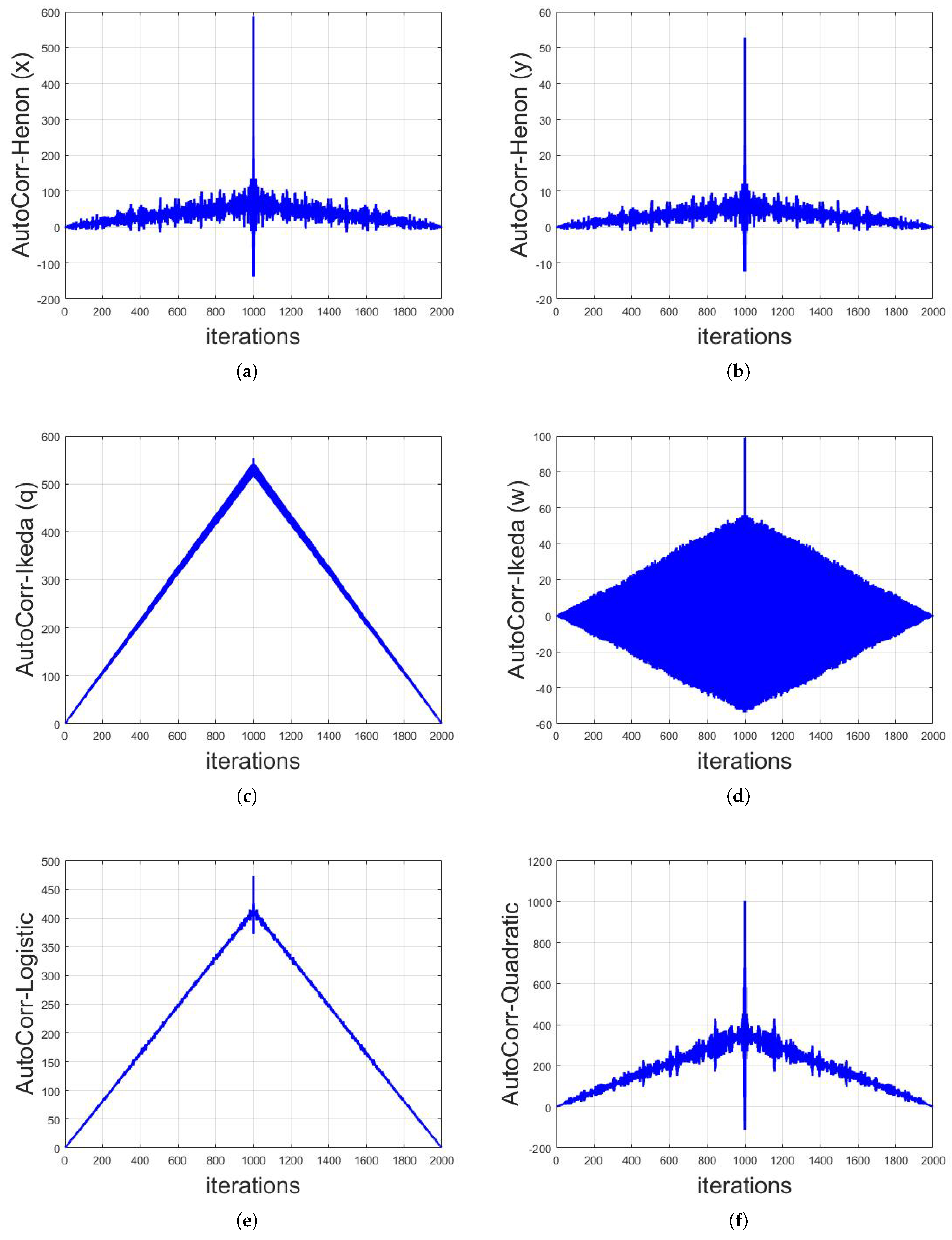
The above defined mathematical structures are applied on long-term sequences of different chaotic maps. The analysis are done based on 1000 iterations of each map with their respective initial values and parameters resulted in 2000 values of correlation. It is shown that, by having the long-term sequence of any chaotic map, the identity of that map can be observed by applying auto-correlation functions, as shown in Figure 6 and Figure 7. It can be seen that the graphs for every chaotic map is different from the other, thus, in the cryptanalysis of chaotic security algorithms, the identity of chaotic map can be revealed as depicted. The identification of chaotic map from the auto-correlation graph can be done by the visual structure and/or numerical values of the graph. For instance, the auto-correlation graph of Logistic map shown in Figure 6e is visually different to the auto-correlation graphs of other chaotic maps and thus can easily be identified. On the contrary, the auto-correlation graphs of Henon x-sequence and Henon y-sequence are visually the same as each other (Figure 6a,b, respectively). However, the numerical values of these two auto-correlation graphs are different from each other and thus can also be differentiated.
It is to be noted that the auto-correlation graphs remain same for a same chaotic map despite the usage of different initial values and parameters. After getting the knowledge of specific chaotic map, the next task is to obtain the initial values and parameters which served as keys. This is achieved by applying statistical analysis of standard deviation and variance, as explained in the next section.
4. Identification of Initial Values
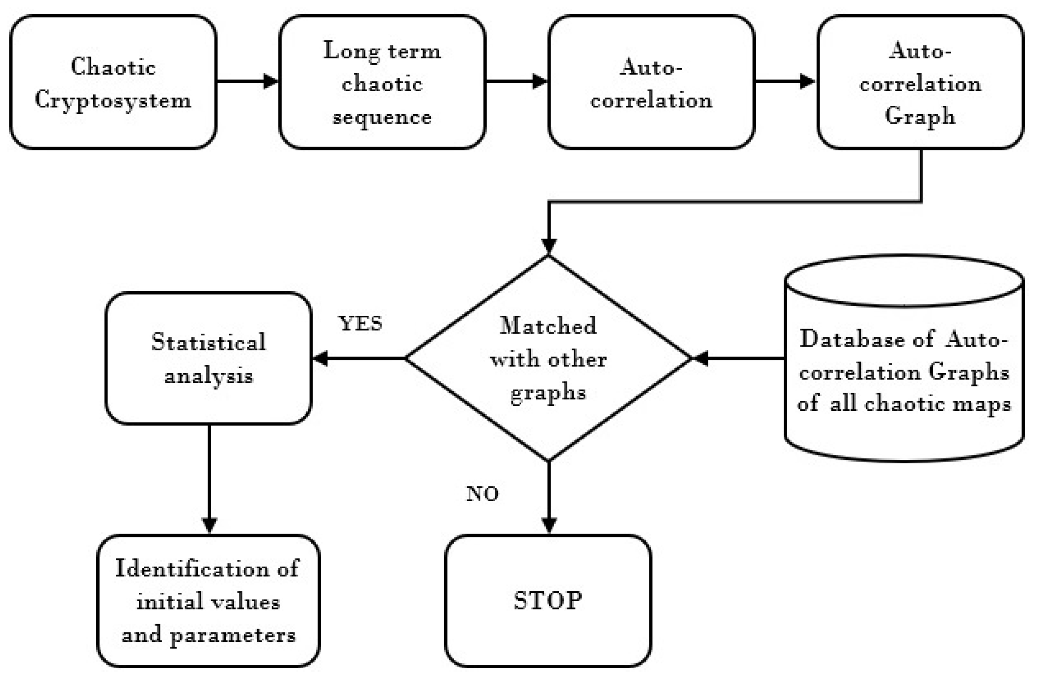
In this paper, it is attempted to analyze the randomness of long-term logistic sequences from a different perspective by performing statistical analysis. We have taken two chaotic maps for the sake of demonstration only and the proposed set of analysis can also be applied to other maps. The details of proposed algorithm in form of block diagram is shown in Figure 8. From the chaotic cryptosystem, the long-term chaotic sequence is obtained. As mentioned above, we have access to the long-term chaotic sequence. Although it would be a much harder task to have access to the long-term sequence of the chaotic map being used, this is out of the scope of the presented work. The auto-correlation of chaotic sequence is calculated and plotted in a graph. Then, this graph is matched with the database of auto-correlation graphs of all chaotic maps. If there is no matched, the algorithm stops. However, in the case of matching one of the maps, the different statistical analysis are applied to identify the initial values and parameters of that specific chaotic map. The simulations and analyses were done using MATLAB R2017a software on Windows 10 platform having Intel Core i5-6200U CPU, 2.30 GHz with RAM of 8.00 GB.
It is worth mentioning here that there is a so-called phenomenon of “dynamical degradation of chaotic properties” when chaotic systems are implemented or simulated on a finite precision machine, for instance a digital computer, which limits the precision and accuracy of the proposed model of the identification of initial values and parameters of chaotic maps. However, we simulated our results considering at least 15 decimal values for the initial parameters (e.g., in case of Logistic map, we considered the initial value of r as 3.854632547852415), which are more than enough regarding the application of cryptography, as the initial values used in those systems have at most of 15 decimal values for the initial parameters. Moreover, the goal of this work was not to identify the “exact” initial values used in cryptography, but to significantly reduce the keyspace to an extent where a brute force attack can be practically possible.
4.1. Initial Values for Logistic Map
As mentioned in Equation (4), the Logistic map sequence depends upon the initial values of two parameters, i.e., r and and our goal is to identify these initial values of Logistic chaotic map. However, in Figure 5, if we do have the access to the long-term chaotic sequence, e.g., 1000 values of sequence, i.e., , it is a simple and straightforward task to get using Equation (4) with the help of . Therefore, the concentration is only on the identification of the value of r employed.
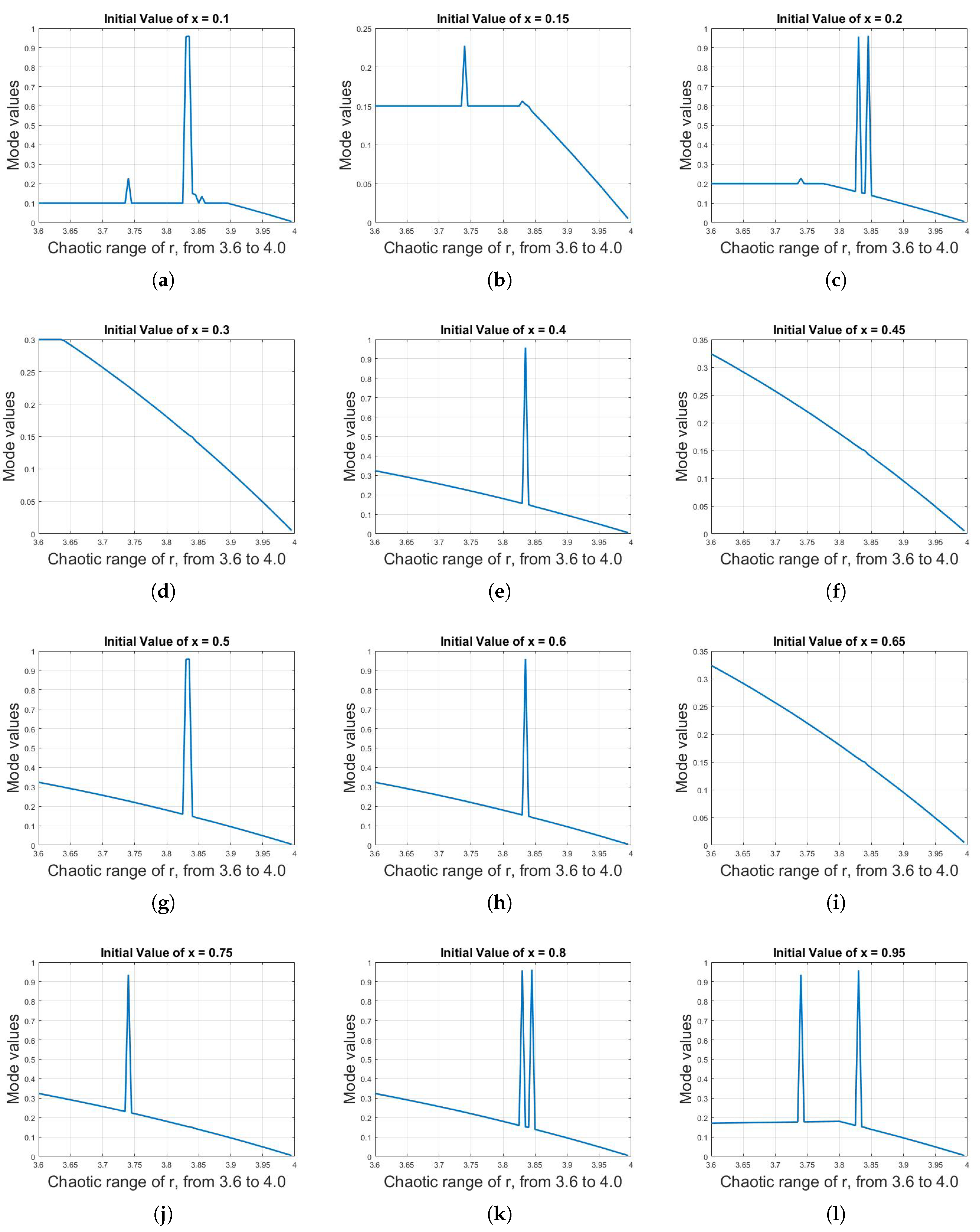
To do so, first, the mean, median and mode analysis are done on the long-term sequences of logistic map; it was observed that the mean is almost same despite different values of parameter r, as were the median and mode analyses. To illustrate this effect, Figure 9 shows the median values of logistic map for different initial values of x against r with the range of 3.6–4.0. Although the median values fluctuate in the range of 0.45–0.75 against r , there is no linear trend (increasing or decreasing), making it a difficult task to assign distinct median values to distinct values of r. Figure 10 shows the mode values of logistic map for different initial values of x against r with the range of 3.6–4.0. The condition is even worse in this case, as, compared to median analysis, not only is there no linear trend but the mode values are also not constant for different initial values of x.
The variance along with the standard deviation are the only two analyses that were found to give somehow different and partially unique values against different values of parameter r.
The term wariance was first coined by Fisher [46]. The variance of group of numeric data tells how far the numeric data are spread out. Mathematically, it is defined as:
where is the value of logistic map iteration at ith index, is the mean and n is the total number of numeric data or iterations in this case.
4.1.1. Setting Number of Iterations n
The variance analysis was applied on the chaotic sequences of logistic map. The simulation results show that the variance of large data of chaotic sequence for a fixed value of parameter r is the same despite different initial values of x. This effect is demonstrated in Figure 11a, where the plot of variance values of logistic sequence of 5000 iterations for a 3.7 value of r against different initial values of x is shown. It can be seen that the variance remains almost the same for each and every initial value of x.
However, if the number of iterations decreases, then there will be variation between the variance values for different initial values of x. Figure 11b shows the plot of variance values of logistic sequences of 50 iterations for a 3.7 value of r against different initial values of x. It can be seen that there is a variation between the variance values. It was observed through different simulation results that at least 1200 iterations would be needed to illustrate an almost constant value of variance.
4.1.2. Variance against Parameter r
After setting a fixed number of iterations on which the values of variance for different initial values of x is same, variance for different values of parameter r is calculated as:
The variance against r was calculated, as shown in Figure 12. The variance values of logistic sequence of 1200 iterations for a 0.5 initial value of x against different values of parameter r are plotted. It can be seen that the variance for different values of r are different and partially unique, as depicted below:
Based on the above equation, we can categorized the variance values of logistic sequence against the parameter r, as shown in Table 1.
In Table 1, if the value of parameter r lies within 3.60–3.73, the variance of generated logistic sequence of 1200 iterations from this range of r with any initial value of x will lie within 0.04–0.05. Thus, if someone can extract 1200 iterations, he/she can easily access the value of r by just examining the variance values. In cryptography, as stated above, the cryptographic algorithm is public and only the keys are private and, in the cryptographic algorithm involving logistic map, the keys are the initial value of x and value of parameter r. The initial value of x does not matter that much, as it changes on each iteration. By assuming that, if someone got the access of 1200 iterations, the current iteration value of x is itself a key, the only key involved is then the value of parameter r.
In Table 1, it can be seen that, by examining values of variance, one can know the range of r, which is used as a key. Although it might not tell exactly the value of r used (i.e., the used value might be r = 3.645321908), but it can certainly reduce the key space by a large margin and then, simply by the brute force attack, one can easily break the cryptographic algorithm.
In Table 1, there are four major regions of variance. The first two regions are unique. If the value of variance lies within in either of these two regions, the corresponding range of r will be unique and can be determined. However, the last two regions overlap with each other. Both regions have almost the same variance range of 0.085–0.110. If the variance of 1200 iterations lies within this range, then it will be difficult to tell to which corresponding value of r they belong.
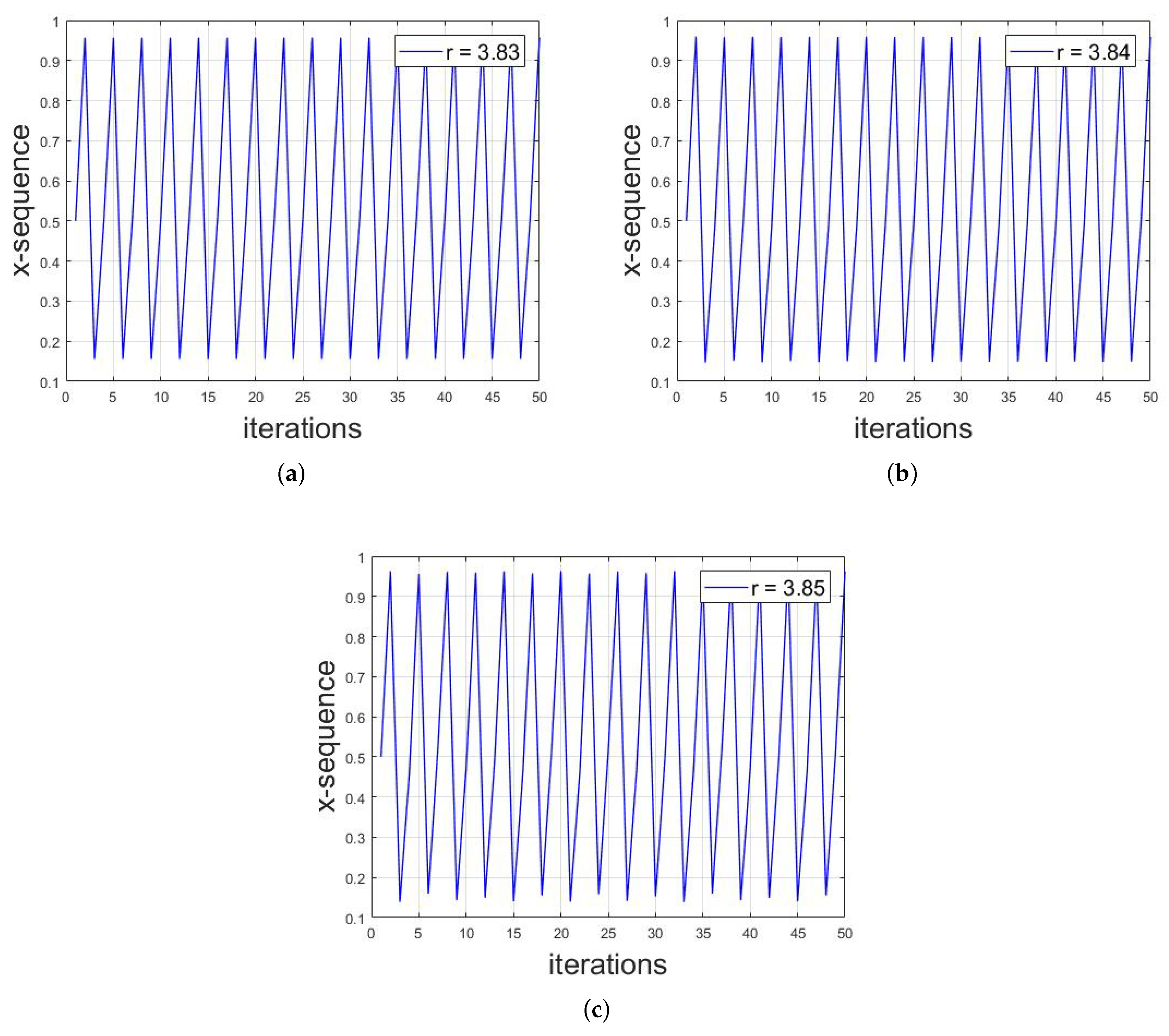
The third region is a small one with the range of r 3.825–3.860. It is an interesting observation that the logistic sequence for the parameter r = 3.825–3.860 behaves periodically, while the other region does not. Figure 13 shows the bifurcation diagram of logistic map for r = 3.825–3.860. In addition, the periodicity of logistic map for this range is shown in Figure 14a–c for and , respectively. Thus, if the variance lies within either Region 3 or Region 4, the decision will be based on the periodicity of that region. If there is periodicity in the sequence, then it belongs to Region 3, otherwise to Region 4.
4.2. Initial Values of Lorenz System
The term standard deviation was first coined by Fisher [46]. The standard deviation of group of numeric data tells how far the numeric data are spread out. Mathematically, it is defined as:
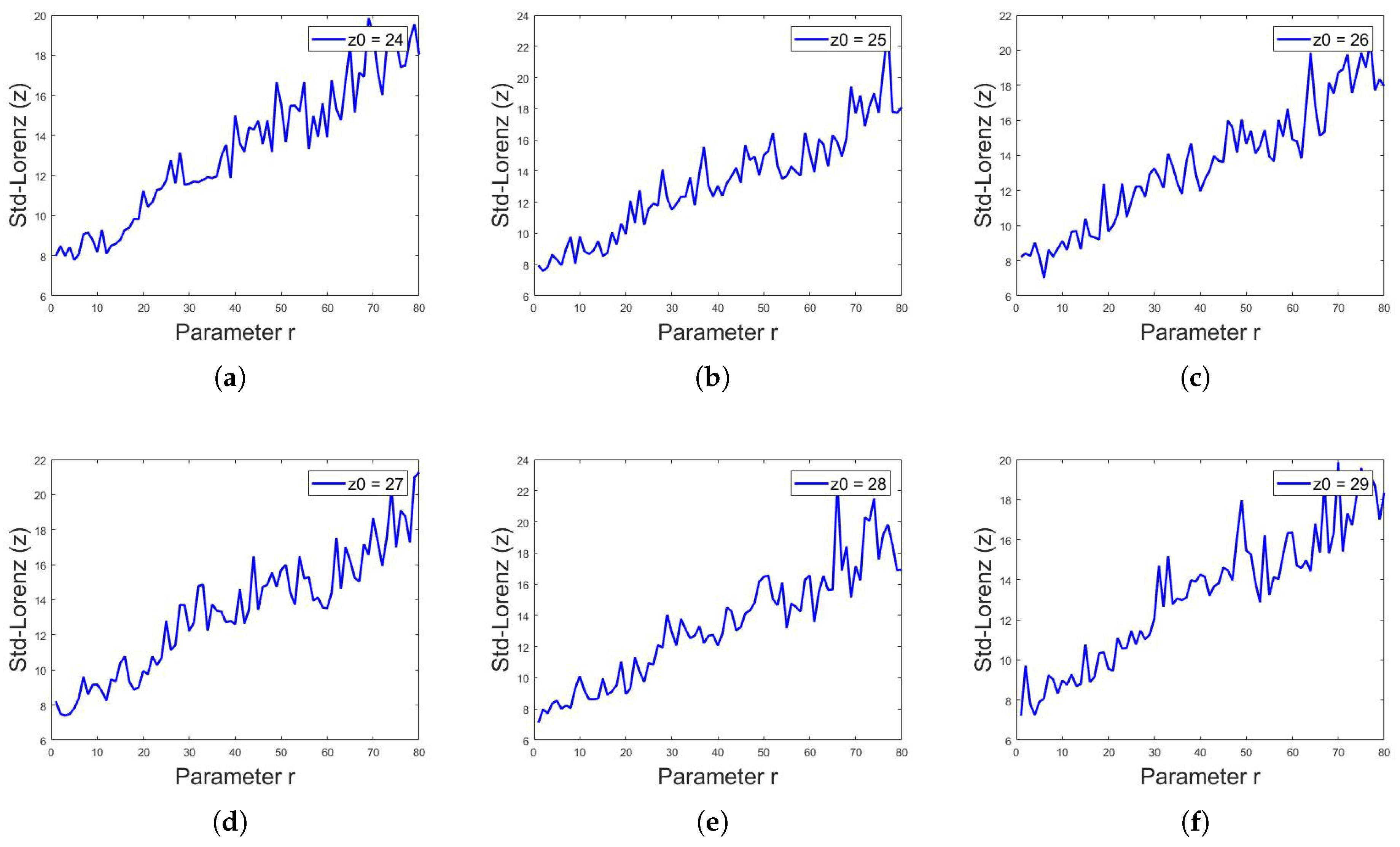
where is the value of Lorenz system iteration at ith index, is the mean and n is the total number of numeric data or iterations in this case. The above defined analyses were applied on and z sequences of Lorenz system for different values of r. As stated above, for , the Lorenz system shows chaotic behavior; cryptographers use the value of r in this chaotic region of as a key along with the initial values of and z. Assuming that, if someone has access to 1000 or more iterations of sequences, the current value of iteration is itself a key regarding the initial values of and z, thus the only key that matters is the value of r being used. It was observed that the standard deviation for the 1000 iterations of any sequence of Lorenz system is different for different values of r, as shown in Table 2. Figure 15, Figure 16 and Figure 17 show the standard deviation of Lorenz system for x sequence, y sequence and z sequence, respectively. The standard deviation is the same for a single sequence despite different initial conditions. The standard deviation is computed from to with the interval of . Mathematically, the standard deviation of sequences of Lorenz system from to can be expressed as:
In addition, the value of standard deviation for all sequences of Lorenz system can be approximately written as the function of parameter r, such that
where is a constant. Thus, by looking at the standard deviation values and having the long-term sequence of Lorenz system, one can easily observe the value of r being used, indirectly shortening the key space or even breaking it in shorter computer time.
5. Conclusions
Based on the results and analysis done, it is concluded that there is a major loophole in chaotic communication symmetric security systems. Taking into account the security algorithm is public, only the key is private and the keys involved in chaotic cryptosystems are the initial values and parameters of chaotic maps. The keyspace can be shortened by applying the proposed method of statistical analysis or can even break in short computer times. Security engineers and mathematical cryptographers do take this effect into consideration when proposing new schemes based on chaotic maps.
Similar to all new proposals, we strongly encourage the analysis of our framework before its immediate deployment for cryptanalysis. The proposed work is a general framework intended for the identification of initial values and parameters. Although the proposed analyses are performed only on Lorenz system and Logistic map, it can be applied on other chaotic maps as well to demonstrate the same effects. Moreover, future research can be conducted to obtain and assess the long-term chaotic sequence from cryptosystems.
Author Contributions
The design problem and proposed methodology were result of the contributions of both the authors. The initial draft of the manuscript was prepared by I.H. The final draft and simulations were done by A.A.
Funding
This research received no external funding.
Acknowledgments
The publication of this article was funded by the Qatar National Library.
Conflicts of Interest
The authors declare no conflict of interest.
References
- Cheng, C.-K.; Chao, P.C.-P. Chaotic Synchronizing Systems with Zero Time Delay and Free Couple via Iterative Learning Control. Appl. Sci. 2018, 8, 177. [Google Scholar] [CrossRef]
- Shukla, P.K.; Khare, A.; Rizvi, M.A.; Stalin, S.; Kumar, S. Applied Cryptography Using Chaos Function for Fast Digital Logic-Based Systems in Ubiquitous Computing. Entropy 2015, 17, 1387–1410. [Google Scholar] [CrossRef] [Green Version]
- T-Herrera, E.J.; Karp, J.; Távora, M.; Santos, L.F. Realistic Many-Body Quantum Systems vs. Full Random Matrices: Static and Dynamical Properties. Entropy 2016, 18, 359. [Google Scholar] [CrossRef]
- Boeing, G. Visual Analysis of Nonlinear Dynamical Systems: Chaos, Fractals, Self-Similarity and the Limits of Prediction. Systems 2016, 4, 37. [Google Scholar] [CrossRef]
- Ahmed, F.; Anees, A.; Abbas, V.U.; Siyal, M.Y. A Noisy Channel Tolerant Image Encryption Scheme. Wirel. Pers. Commun. 2014, 77, 2771–2791. [Google Scholar] [CrossRef]
- Ahmed, F.; Anees, A. Hash-Based Authentication of Digital Images in Noisy Channels. In Robust Image Authentication in the Presence of Noise; Springer: Cham, Switzerland, 2015; pp. 1–42. [Google Scholar]
- Bolle, R.M.; Pankanti, S.; Ratha, N.K. Evaluation Techniques for Biometrics-Based Authentication Systems (FRR). In Proceedings of the 15th International Conference on Pattern Recognition, 3–7 September 2000; Volume 2, pp. 2831–2837. [Google Scholar]
- Dass, S.C.; Zhu, Y.; Jain, A.K. Validating a Biometric Authentication System: Sample Size Requirements; Technical Report MSU-CSE-05-23; Department of Computer Science and Engineering (CSE), Michigan State University: East Lansing, MI, USA, 2005. [Google Scholar]
- Jain, A.K.; Hong, L.; Bolle, R. On-Line Fingerprint Verification. IEEE Trans. Pattern Recognit. Mach. Intell. 1997, 19, 302–314. [Google Scholar] [CrossRef]
- Behnia, S.; Akhshani, A.; Mahmodi, H.; Akhavan, A. A novel algorithm for image encryption based on mixture of chaotic maps. Chaos Solitons Fractals 2008, 35, 408–419. [Google Scholar] [CrossRef]
- Liu, H.; Wang, X. Color image encryption based on one-time keys and robust chaotic maps. Comput. Math. Appl. 2010, 59, 3320–3327. [Google Scholar] [Green Version]
- Anees, A.; Siddiqui, A.M.; Ahmed, F. Chaotic substitution for highly autocorrelated data in encryption algorithm. Commun. Nonlinear Sci. Numer. Simul. 2014, 19, 3106–3118. [Google Scholar] [CrossRef]
- Anees, A.; Siddiqui, A.M.; Ahmed, J.; Hussain, I. A technique for digital steganography using chaotic maps. Nonlinear Dyn. 2014, 75, 807–816. [Google Scholar] [CrossRef]
- Gondal, M.A.; Anees, A. Analysis of optimized signal processing algorithms for smart antenna system. Neural Comput. Appl. 2013, 23, 1083–1087. [Google Scholar] [CrossRef]
- Anees, A.; Khan, W.A.; Gondal, M.A.; Hussain, I. Application of Mean of Absolute Deviation Method for the Selection of Best Nonlinear Component Based on Video Encryption. Zeitschrift für Naturforschung A 2013, 68, 479–482. [Google Scholar] [CrossRef] [Green Version]
- Anees, A.; Ahmed, Z. A Technique for Designing Substitution Box Based on Van der Pol Oscillator. Wirel. Pers. Commun. 2015, 82, 1497–1503. [Google Scholar] [CrossRef]
- Anees, A.; Gondal, M.A. Construction of Nonlinear Component for Block Cipher Based on One-Dimensional Chaotic Map. 3D Res. 2015, 6. [Google Scholar] [CrossRef]
- Anees, A.; Siddiqui, A.M. A technique for digital watermarking in combined spatial and transform domains using chaotic maps. In Proceedings of the IEEE 2nd National Conference on Information Assurance (NCIA), Rawalpindi, Pakistan, 11–12 December 2013; pp. 119–124. [Google Scholar]
- Ansari, K.J.; Ahmad, I.; Mursaleen, M.; Hussain, I. On Some Statistical Approximation by (p,q)-Bleimann, Butzer and Hahn Operators. Symmetry 2018, 10, 731. [Google Scholar] [CrossRef]
- Vieira, R.S.S.; Michtchenko, T.A. Relativistic chaos in the anisotropic harmonic oscillator. Chaos Solitons Fractals 2018, 117, 276–282. [Google Scholar] [CrossRef]
- Doroshin, A.V. Chaos as the hub of systems dynamics. The part I—The attitude control of spacecraft by involving in the heteroclinic chaos. Commun. Nonlinear Sci. Numer. Simul. 2018, 59, 47–66. [Google Scholar] [CrossRef]
- Guzzo, M.; Lega, E. Geometric chaos indicators and computations of the spherical hypertube manifolds of the spatial circular restricted three-body problem. Phys. D Nonlinear Phenom. 2018, 373, 38–58. [Google Scholar] [CrossRef]
- Alves, P.R.L.; Duarte, L.G.S.; da Mota, L.A.C.P. Detecting chaos and predicting in Dow Jones Index. Chaos Solitons Fractals 2018, 110, 232–238. [Google Scholar] [CrossRef]
- Cairone, F.; Anandan, P.; Bucolo, M. Nonlinear systems synchronization for modeling two-phase microfluidics flows. Nonlinear Dyn. 2018, 92, 75–84. [Google Scholar] [CrossRef]
- Lorenz, E.N. Deterministic Nonperiodic Flow. J. Atmos. Sci. 1963, 20, 130–141. [Google Scholar] [CrossRef] [Green Version]
- Akhmet, M.U.; Fen, M.O. Entrainment by Chaos. J. Nonlinear Sci. 2014, 24, 411–439. [Google Scholar] [CrossRef]
- Kaslik, E.; Balint, Ş. Chaotic Dynamics of a Delayed Discrete Time Hopfield Network of Two Nonidentical Neurons with no Self-Connections. J. Nonlinear Sci. 2008, 18, 415–432. [Google Scholar] [CrossRef]
- Buscarino, A.; Fortuna, L.; Frasca, M. Experimental robust synchronization of hyperchaotic circuits. Phys. D Nonlinear Phenom. 2009, 238, 1917–1922. [Google Scholar] [CrossRef]
- Hussain, I.; Anees, A.; Aslam, M.; Ahmed, R.; Siddiqui, N. A noise resistant symmetric key cryptosystem based on S8 S-boxes and chaotic maps. Eur. Phys. J. Plus 2018, 133, 1–23. [Google Scholar] [CrossRef]
- Hussain, I.; Anees, A.; AlKhaldi, A.H.; Algarni, A.; Aslamd, M. Construction of chaotic quantum magnets and matrix Lorenz systems S-boxes and their applications. Chin. J. Phys. 2018, 56, 1609–1621. [Google Scholar] [CrossRef]
- Hussain, I.; Anees, A.; Algarni, A. A novel algorithm for thermal image encryption. J. Integr. Neurosci. 2018, 17, 447–461. [Google Scholar] [CrossRef] [PubMed]
- Anees, A. An Image Encryption Scheme Based on Lorenz System for Low Profile Applications. 3D Res. 2015, 6, 1–10. [Google Scholar] [CrossRef]
- Kocarev, L. Chaos-based cryptography: A brief overview. IEEE Circuits Syst. Mag. 2001, 1, 6–21. [Google Scholar] [CrossRef]
- Shannon, C.E. Communication Theory of Secrecy Systems. Bell Syst. Tech. J. 1949, 28, 656–715. [Google Scholar] [CrossRef]
- Sobhy, M.I.; Shehata, A.-E.R. Methods of attacking chaotic encryption and countermeasures. In Proceedings of the IEEE International Conference on Acoustics, Speech, and Signal Processing, Salt Lake City, UT, USA, 7–11 May 2001; Volume 2, pp. 1001–1004. [Google Scholar]
- Hussain, I.; Gondal, M.A. An extended image encryption using chaotic coupled map and S-box transformation. Nonlinear Dyn. 2014, 76, 1355–1363. [Google Scholar] [CrossRef]
- Jamal, S.S.; Shah, T.; Hussain, I. An efficient scheme for digital watermarking using chaotic map. Nonlinear Dyn. 2013, 73, 1469–1474. [Google Scholar] [CrossRef]
- Daemen, J.; Rijmen, V. The Design of RijndaeL: AES—The Advanced Encryption Standard; Springer: New York, NY, USA, 2002. [Google Scholar]
- Khan, M.; Shah, T.; Mahmood, H.; Gondal, M.A.; Hussain, I. A novel technique for the construction of strong S-boxes based on chaotic Lorenz systems. Nonlinear Dyn. 2012, 70, 2303–2311. [Google Scholar] [CrossRef]
- Jakimoski, G.; Kocarev, L. Chaos and Cryptography: Block Encryption Ciphers Based on Chaotic Maps. IEEE Trans. Circuits Syst. I Fundam. Theory Appl. 2001, 48, 163–169. [Google Scholar] [CrossRef]
- Verhulst, P.F. Recherches mathématiques sur la loid’accroissement de la population. Nouv. Mem. Acad. R. Sci. B.-Lett. Brux 1845, 18, 1–41. [Google Scholar]
- May, R.M. Biological populations with non overlapping generations, stable points, stable cycles, and chaos. Science 1974, 186, 645–647. [Google Scholar] [CrossRef] [PubMed]
- May, R.M. Biological populations obeying difference equations, stable points, stable cycles, and chaos. J. Theor. Biol. 1975, 51, 511–524. [Google Scholar] [CrossRef]
- May, R.M. Simple mathematical models with very complicated dynamics. Nature 1976, 261, 459–467. [Google Scholar] [CrossRef]
- Oppenheim, A.V.; Schafer, R.W. Discrete-Time Signal Processing, 3rd ed.; Prentice Hall Signal Processing: Upper Saddle River, NJ, USA, 2009. [Google Scholar]
- Fisher, R.A. The Correlation Between Relatives on the Supposition of Mendelian Inheritance. Trans. R. Soc. Edinb. 1918, 52, 399–433. [Google Scholar] [CrossRef]
Figure 1.
The illustration of the application considered in this work; basic communication model of symmetric cryptography.
Figure 1.
The illustration of the application considered in this work; basic communication model of symmetric cryptography.

Figure 2.
Numerical solution of Lorenz system with initial values of and constant values of and for: (a) structure; (b) structure; and (c) structure.
Figure 2.
Numerical solution of Lorenz system with initial values of and constant values of and for: (a) structure; (b) structure; and (c) structure.

Figure 3.
(a) The individual x-sequence against number of iterations with initial conditions of . (b) Sensitive dependence of initial conditions: the plot for x-sequence with initial conditions of as well as the plot for x-sequence with initial conditions of . It can be seen that the two sequences completely differ apart after 1300 iterations, despite of the difference in one of the initial conditions by a margin of 0.00000001.

Figure 4.
(a) The individual x-sequence against number of iterations with initial conditions of . (b) Sensitive dependence of initial conditions; shows the plot for x-sequence with initial conditions of as well as the plot for x-sequence with initial conditions of . It can be seen that the two sequences completely differ apart after 75 iterations despite the difference in one of the initial conditions by a margin of 0.000000001.

Figure 5.
Proposed framework for identifying the initial values of chaotic maps using three steps: accessing the long term chaotic sequence, identification of the type of chaotic map using auto-correlation graphs and identification of the initial values using different statistical analysis.
Figure 5.
Proposed framework for identifying the initial values of chaotic maps using three steps: accessing the long term chaotic sequence, identification of the type of chaotic map using auto-correlation graphs and identification of the initial values using different statistical analysis.

Figure 6.
Auto-correlation graphs of different chaotic maps with their respective initial conditions and parameters taken on 1000 iterations: (a) Henon chaotic map x-sequence; (b) Henon chaotic map y-sequence; (c) Ikeda chaotic map q-sequence; (d) Ikeda chaotic map w-sequence; (e) Logistic map; and (f) Quadratic map.

Figure 7.
Auto-correlation graphs of different chaotic maps with their respective initial conditions and parameters taken on 1000 iterations: (a) Lorenz chaotic map x-sequence; (b) Lorenz chaotic map y-sequence; (c) Lorenz chaotic map z-sequence; (d) Rossler chaotic map e-sequence; (e) Rossler chaotic map q-sequence; and (f) Rossler chaotic map w-sequence.

Figure 8.
The top-level block diagram of proposed work.

Figure 9.
(a)–(l) Median values of logistic map for different initial values of x against r with the range of 3.6–4.0. Although the median values fluctuate in the range of 0.45–0.75 against r, there is no linear trend (increasing or decreasing), making it a difficult task to assign distinct median values to distinct values of r.

Figure 10.
(a)–(l) Mode values of logistic map for different initial values of x against r with the range of 3.6–4.0. The condition is even worse in this case as compared to median analysis; not only is there no linear trend but the mode values are also not constant for different initial values of x.

Figure 11.
(a) Plot of variance values of 5000 logistic sequence iterations for 3.7 value of r against different initial values of x, where the variance remains almost the same for each and every initial value of x. (b) The plot of variance values of logistic sequences of 50 iterations for a 3.7 value of r against different initial values of x. It can be seen that there is a variation between the variance values in this case.

Figure 12.
(a)–(l) Plot of variance values of 1200 logistic sequence iterations for 0.5 value of x against different values of parameter r. The variance for different values of r are different and partially unique.
Figure 12.
(a)–(l) Plot of variance values of 1200 logistic sequence iterations for 0.5 value of x against different values of parameter r. The variance for different values of r are different and partially unique.

Figure 13.
Bifurcation diagram of logistic map for r = 3.825–3.860.

Figure 14.
Illustration of periodicity of logistic map for (a) ; (b) and (c) .

Figure 15.
Standard deviation of Lorenz system for x sequence, with initial values of and constant values of and , showing different values of standard deviation for different values of r, for in (a–f), respectively.
Figure 15.
Standard deviation of Lorenz system for x sequence, with initial values of and constant values of and , showing different values of standard deviation for different values of r, for in (a–f), respectively.

Figure 16.
Standard deviation of Lorenz system for y sequence, with initial values of and constant values of and , showing different values of standard deviation for different values of r, for in (a–f), respectively.
Figure 16.
Standard deviation of Lorenz system for y sequence, with initial values of and constant values of and , showing different values of standard deviation for different values of r, for in (a–f), respectively.

Figure 17.
Standard deviation of Lorenz system for y sequence, with initial values of and constant values of and , showing different values of standard deviation for different values of r, for in (a–f), respectively.
Figure 17.
Standard deviation of Lorenz system for y sequence, with initial values of and constant values of and , showing different values of standard deviation for different values of r, for in (a–f), respectively.


Table 1.
Variance range against parameter r range.
| Region | Variance Range | Parameter, r Range |
|---|---|---|
| 1 | 0.039–0.050 | 3.60–3.73 |
| 2 | 0.050–0.085 | 3.73–3.82 |
| 3 | 0.085–0.110 | 3.82–3.86 |
| 4 | 0.085–0.118 | 3.86–3.99 |
Table 2.
Standard deviation values of Lorenz system for x, y and z sequences against parameter r range.
Table 2.
Standard deviation values of Lorenz system for x, y and z sequences against parameter r range.
| r | x | y | z | r | x | y | z |
|---|---|---|---|---|---|---|---|
| 24 | 5.9721 | 6.8049 | 7.5644 | 44 | 10.4401 | 13.7855 | 14.8617 |
| 26 | 6.5186 | 7.2033 | 6.1305 | 46 | 10.6639 | 13.7069 | 13.3215 |
| 28 | 7.9851 | 9.1540 | 8.2105 | 48 | 10.9514 | 14.2571 | 14.6004 |
| 30 | 7.7617 | 9.0118 | 7.8162 | 50 | 11.5522 | 14.7872 | 13.4296 |
| 32 | 8.8601 | 10.3146 | 9.1604 | 52 | 11.6983 | 15.5916 | 14.7479 |
| 34 | 8.9962 | 10.5397 | 9.4619 | 54 | 12.0774 | 15.6581 | 13.7141 |
| 36 | 9.4806 | 11.0827 | 9.3204 | 56 | 12.1455 | 15.9730 | 13.9568 |
| 38 | 9.7408 | 11.4435 | 9.7575 | 58 | 12.3523 | 16.5226 | 14.4226 |
| 40 | 10.0324 | 12.6311 | 12.7988 | 60 | 12.8113 | 17.6593 | 16.2303 |
| 42 | 10.2070 | 13.1060 | 13.7087 | 62 | 13.0964 | 18.1885 | 16.5554 |
© 2019 by the authors. Licensee MDPI, Basel, Switzerland. This article is an open access article distributed under the terms and conditions of the Creative Commons Attribution (CC BY) license (http://creativecommons.org/licenses/by/4.0/).
Share and Cite
MDPI and ACS Style
Anees, A.; Hussain, I. A Novel Method to Identify Initial Values of Chaotic Maps in Cybersecurity. Symmetry 2019, 11, 140. https://0-doi-org.brum.beds.ac.uk/10.3390/sym11020140
AMA Style
Anees A, Hussain I. A Novel Method to Identify Initial Values of Chaotic Maps in Cybersecurity. Symmetry. 2019; 11(2):140. https://0-doi-org.brum.beds.ac.uk/10.3390/sym11020140
Chicago/Turabian StyleAnees, Amir, and Iqtadar Hussain. 2019. "A Novel Method to Identify Initial Values of Chaotic Maps in Cybersecurity" Symmetry 11, no. 2: 140. https://0-doi-org.brum.beds.ac.uk/10.3390/sym11020140
Note that from the first issue of 2016, this journal uses article numbers instead of page numbers. See further details here.