A Programming-Based Algorithm for Probabilistic Uncertain Linguistic Intuitionistic Fuzzy Group Decision-Making

Abstract

As an effective tool to express the subjective preferences of decision makers, the linguistic term sets (LTS) have been widely used in group decision-making (GDM) problems, such as hesitant fuzzy LTS, linguistic hesitant fuzzy sets, probabilistic LTS, etc. However, due to the increasing complexity of practical decision-making (DM) problems, LTS still has a lot of room to expand in fuzzy theory. Qualitative uncertainty information in the application of GDM is yet to be improved. Therefore, in order to improve the applicability of linguistic terms in DM problems, a probabilistic uncertain linguistic intuitionistic fuzzy set (PULIFS) that can fully express the decision-maker’s (DM’s) evaluation information is first proposed. To improve the rationality of DM results, we give a method for determining individual weights in the probabilistic uncertain linguistic intuitionistic fuzzy preference relation (PULIFPR) environment. In addition, we present two consistency definitions of PULIFPR to reflect both the assessment information and risk attitudes of decision makers. Subsequently, a series of goal programming models (GPMs) are established, which effectively avoid the consistency check and correction process of existing methods. Finally, the developed method is applied to an empirical example concerning the selection of a virtual reality (VR) project. The advantages of the proposed method are demonstrated by comparative analysis.

1. Introduction

Because of the inherent subjective ambiguity of human thinking and the complexity of practical decision-making (DM) problems, the use of qualitative information is almost an indispensable link in DM. As the most commonly used qualitative information expression tool, linguistic terms (LT) have been extensively studied by scholars. Since Zadeh [1] proposed linguistic variables in 1975, various extended forms of LT have been proposed to model qualitative information and improve its calculation. In order to have a general understanding of these extended LT, we will present the general development process of LT in the form of

Table 1. A brief history of the types of linguistic terms.

	Year	Event
Traditional	1975	Zadeh proposes the linguistic variable and introduced the fuzzy linguistic approach [1,2,3].
linguistic	1981	Yager presents an ordered structure model [4].
models	1988	Degani and Bortolan present the semantic model [5].
	1993	Delgado and Verdegay propose the symbolic model [6].
	2000	Herrera and Martinez introduce the two-tuple linguistic model [7].
	2004	Xu defines the virtual linguistic model [8].
Complex	2004	Xu introduces the uncertain linguistic term (ULT) [9].
linguistic	2012	Rodriguez et al. present the concept of hesitant fuzzy linguistic term sets (HFLTS) [10].
expression	2014	Meng et al. propose the linguistic hesitant fuzzy sets (LHFS) [11].
	2014	Zhang gives the concept of linguistic intuitionistic fuzzy sets (LIFS) [12].
	2015	Ye presents the single-valued neutrosophic linguistic sets (SVNLS) [13].
	2016	Pang et al. present the probabilistic linguistic term sets (PLTS) [14].
	2107	Lin et al. define the probabilistic uncertain linguistic term sets (PULTS) [15].
	2018	Bai et al. present the interval-valued probabilistic linguistic term sets (IVPLTS) [16].
	2018	Zhang et al. propose the dual hesitant fuzzy linguistic term sets (DHFLTS) [17].

.

It is easy to see from the Table 1 that the development of LT can be mainly divided into two stages. The first stage is some traditional linguistic models, whose main research object is single LT. The second stage is the complex linguistic expression stage, whose linguistic information expression form is generally more than one LT or implied multiple linguistic information. In addition, it is easy to find that the LT of the later stage mostly introduces probability to comprehensively reflect the subjective uncertainty of decision makers (DMs) and the randomness of objective existence. All of these proposed sets give expression methods of qualitative information from different perspectives, and all of them have been applied reasonably in the DM problem. However, the qualitative information expressed by these sets has different degrees of defects. For example, although probabilistic uncertain linguistic term sets (PULTS) expresses the DM’s preference information and its probability distribution, it fails to consider the DM’s non-preference information, while linguistic intuitionistic fuzzy sets (LIFS) only expressed the subjective hesitation of DMs from the perspective of preference and non-preference, failing to consider the probability distribution of its information. Therefore, in order to improve the expression of qualitative information and promote the use of LT in DM problems, this paper further proposes a probabilistic uncertain linguistic intuitionistic fuzzy set (PULIFS) based on the above research, which integrates the advantages of LIFS and PULTS.

For example, when a decision team needs to evaluate and compare some alternatives, due to the complexity of the actual decision-making environment, the decision-makers can only provide qualitative preference and non-preference information based on the linguistic term set (LTS) S = {$s_0$: extremely poor, $s_1$: very poor, $s_2$: poor, $s_3$: slightly poor, $s_4$: fair, $s_5$: slightly good, $s_6$: good, $s_7$: very good, $s_8$: extremely good}. Among them, 40% of the DMs gave preference information between the very poor and the slightly poor, and the non-preference information was between the fair and the slightly good. While 60% of DMs gave preference information between fair and good, and non-preference information was between very poor and poor. Then the preference information given by this decision team can be represented by PULIFS as

$$P=\{\langle ([s_1,s_3],[s_4,s_5]),0.4\rangle ,\langle ([s_4,s_6],[s_1,s_2]),0.6\rangle \}$$

From the above example, it can be seen that PULIFSs not only expresses the qualitative preference and non-preference information of DMs, but also provides flexible linguistic selection space for DMs and gives the probability distribution information of an uncertain linguistic. Moreover, the above example is only one application case of PULIFS proposed, besides, PULIFS can also be used to express individual preference information. So it is natural that we want to apply PULIFS to group decision-making (GDM) problems to compensate for the application limitations of existing sets, thus improving the application of qualitative information in fuzzy theory. This is the first focus of this paper.

Considering the cognitive uncertainty and fuzziness of DMs in complex decision-making environment, the application of uncertainty theory in decision-making has been widely studied. For example, Pamucar et al. [18] combined with linguistic neutrosophic numbers presented the selection method of power generation technology, and Liu et al. [19] established the selection model of transportation service provider with single valued neutrosophic number. In addition, preference relation (PR) has been widely used in GDM as an effective tool to express DMs’ preferences over alternatives. Its main types include fuzzy PR [20], multiplicative PR [21] and linguistic PR (LPR) [22]. On this basis, many forms of preference relations have been proposed, such as interval fuzzy PR [23], interval multiplicative PR [24], intuitionistic PR [25], intuitionistic multiplicative PR [26], linguistic intuitionistic PR [27], etc. These PRs all express the DM’s preference information in different forms from different perspectives. However, the application of existing PRs in GDM have the following defects:

(1)

Most of the PRs fail to reflect the distribution of information given by DMs.

(2)

Most studies on PRs ignore the information that cannot be grasped by DMs or fail to take into account information loss caused by certain objective factors.

(3)

In the process of solving the priority weights, most of the GPMs only consider the principle of minimum consistency deviation and ignore the risk attitude of decision makers, which may result in the loss of original information and reduce the rationality of the ranking results.

(4)

Almost all methods, none can guarantee the consistency of PRs in the process of solving priority weights. They all need to test and improve the consistency of PRs, which greatly reduces the accuracy of the results.

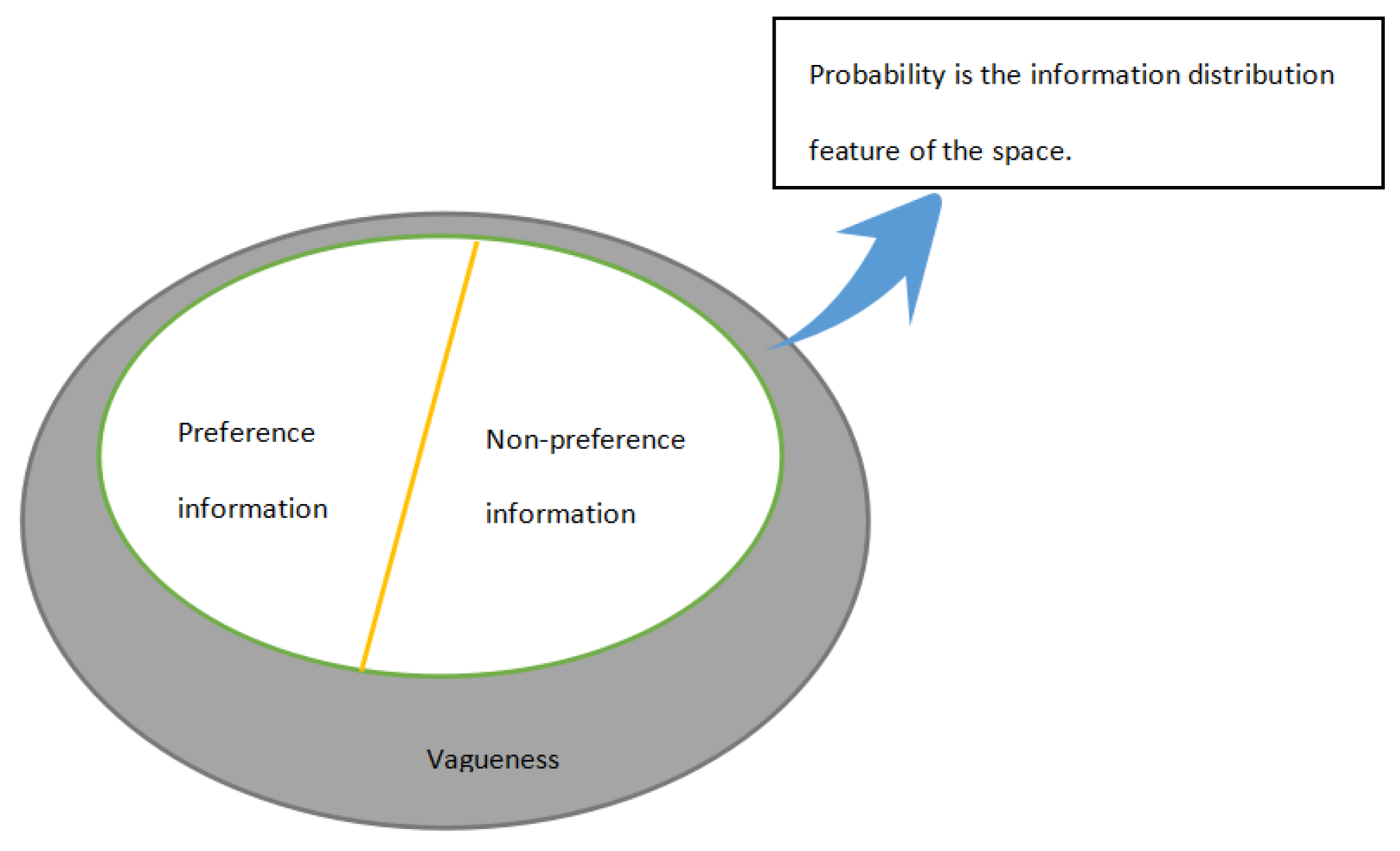
Therefore, in order to make up for the above defects of the existing methods, this paper further proposes probabilistic uncertain linguistic intuitionistic fuzzy preference relation (PULIFPR) based on the excellent nature of PULIFS proposed. To ensure the reasonable application of PR in GDM, we divide the uncertain information represented by PULIFPR into vagueness uncertain information and non-vagueness uncertain information, and its consistency is studied from two spatial dimensions respectively. Among them, non-vagueness uncertain information refers to some relevant information held by the decision maker for the alternatives to be compared. While vagueness uncertain information refers to the decision information that cannot be given by decision makers due to lack of relevant experience and knowledge, or the information loss caused by some objective factors. The non-vagueness uncertainty information in PULIFPR is mainly presented in the form of qualitative preference and non-preference information. For ease of understanding, the relationship between the uncertain information of each dimension expressed by PULIFPR is shown in Figure 1.

From Figure 1, we can see intuitively that the uncertain space of PULIFPR is divided into vagueness subspace and non-vagueness subspace, and non-vagueness subspace can be further divided into preference information and non-preference information. Therefore, this paper will discuss the consistency of PULIFPR from the perspectives of preference, non-preference and vagueness, so as to guarantee the rationality and accuracy of the final results to the greatest extent. We will consider the DM’s risk preference comprehensively based on the consistency proposed, so as to establish a reasonable GPM and get a reasonable ranking result.

Based on the above analysis, the main contributions of this paper is organized as follows:

(1)

We put forward PULIFS, which is of great significance for improving the application of LT in fuzzy theory and effectively promoting the application of qualitative information in GDM.

(2)

We extracted fuzzy and non-fuzzy uncertain information from PULIFPR, and then used it to define the distance measure of PULIFPRs, thus solving the problem of determining the individual weight in GDM.

(3)

We built a series of GPMs by taking into account the DMs’ qualitative preference, non-preference and fuzzy information, and then give a reasonable ranking results of PULIFPR.

(4)

We avoided the consistency test and correction of preference relation in GDM, thus simplifying the process of GDM and improving the accuracy of decision result.

(5)

The proposed method is applied to the industrial docking of virtual reality (VR) industry conference, which solves the problem of project selection before industrial docking.

To sum up, compared with the existing group decision-making methods, the main advantages of the proposed method are as follows:

(1)

Most of the decision-making methods directly use the information provided by the decision-maker to model and make judgments, but ignore the information that the decision-maker fails to grasp or the information loss caused by some objective factors. In this paper, uncertain information is divided into fuzzy uncertain information and non-fuzzy uncertain information for comprehensive discussion, which improves the utilization of information and ensures the rationality of decision-making results.

(2)

Most of the existing decision-making models fail to consider the risk attitude of DMs and fail to guarantee the consistency of preference information given by DMs. In this paper, two extreme attitudes of DMs under uncertain conditions are considered to establish programming models, which ensures the consistency of preference relations, simplifies GDM process and improves the accuracy of decision-making results.

The remainder of this paper is organized as follows: Section 2 recalls some basic concepts, including LIFS, PLTS, PULTS. Section 3 introduces the concepts of PULIFS and PULIFPR, and gives the definition of the distance measure of PULIFSs. Section 4 discusses the consistency of PULIFPR and establishes the corresponding GPM to obtain its comprehensive priority ranking weight. Then a specific algorithm is developed for GDM with PULIFPRs. In Section 5, a practical example about VR industry and comparative analysis are given to demonstrate the proposed method. Finally, Section 6 is concluding remarks.

2. Preliminaries

In this part, we review some basic concepts of LIFS, PLTS and PULTS, and point out the main disadvantage of these fuzzy sets.

2.1. PLTS and PULTS

For convenience, all the LST mentioned in this article are represented by $S=\{s_{\alpha }|\alpha \in [0,2\tau ]\}$ except for special explanations. In order to present the probability distribution information of the HFLTS, Pang et al. [14] proposed PLTS.

Definition 1

([14]). Let $S=\{s_{\alpha }|\alpha \in [0,2\tau ]\}$ be a continuous LTS, then a PLTS is defined as

$$L(p)=\{L^{(k)}(p^{(k)})|L^{(k)}\in S,p^{(k)}\ge 0,k=1,2,\cdots ,\#L(p),\sum _{k=1}^{\#L(p)}{p}^{(k)}\le 1\},$$

(1)

where $L^{(k)}(p^{(k)})$ is the linguistic term $L^{(k)}$ associated with the probability $p^{(k)}$, and $\#L(p)$ is the number of all different linguistic terms in $L(p)$. To further reflect the hesitation of DMs, Lin et al. [15] expanded PLTS into PULTS:

$$S(p)=\{\langle [L^k,U^k],p^k\rangle |p^k\ge 0,k=1,2\cdots ,\#S(p),\sum _{k=1}^{\#S(p)}{p}^k\le 1\},$$

(2)

where $\langle [L^k,U^k],p^k\rangle$ represents the uncertain linguistic variable $[L^k,U^k]$ associated with its probability $p^k$. $L^k,U^k\in S$ are the linguistic terms, $L^k\le U^k$, and $\#S(p)$ is the cardinality of $S(p)$.

2.2. LIFS

To reflect the DM’s qualitative non-preference information, Zhang [12] proposes LIFS.

Definition 2

([12]). Let X be a finite universal set and $S=\{s_{\alpha }|\alpha \in [0,2\tau ]\}$ be a continuous linguistic term set. Then a LIFS L in X is given as

$$L=\{(x,s_{\theta }(x),s_{\sigma }(x))|x\in X\}$$

(3)

where $s_{\theta }(x),s_{\sigma }(x)\in S$ stand for the linguistic membership degree and linguistic nonmembership of the element x to L, respectively, and $0\le \theta +\sigma \le 2\tau$ for all $x\in X$.

PULTS only takes into account the DM’s qualitative preference information and its probability distribution, however, in actual DM, DMs may need to give preference and non-preference information from both sides due to various uncertainties. Although LIFS takes into account the DMs’ non-preference information, it requires the DMs to give only single linguistic terms as decision information, which cannot reflect the decision makers’ hesitation in a complex environment. Therefore, in order to avoid the limitations mentioned above in actual DM, this paper proposes PULIFS in combination with the advantages of PULTS and LIFS.

3. PULIFS and PULIFPR

3.1. PULIFS

Definition 3.

Let $S=\{s_{\alpha }|\alpha \in [0,2\tau ]\}$ be a continuous LTS, then a PULIFS on S is expressed by a mathematical symbol:

$$U(p)=\{\langle ([s_{{\underline{u}}^k},s_{{\overline{u}}^k}],[s_{{\underline{v}}^k},s_{{\overline{v}}^k}]),p^k\rangle |p^k\ge 0,k=1,2\cdots ,\#U(p),\sum _{k=1}^{\#U(p)}{p}^k\le 1\},$$

(4)

where $\langle ([s_{{\underline{u}}^k},s_{{\overline{u}}^k}],[s_{{\underline{v}}^k},s_{{\overline{v}}^k}]),p^k\rangle$ is a PULIF element (PULIFE), which denotes the k-th uncertain linguistic intuitionistic variable (ULIV) $([s_{{\underline{u}}^k},s_{{\overline{u}}^k}],[s_{{\underline{v}}^k},s_{{\overline{v}}^k}])$ associated with its probability $p^k$ in $U(p)$, and $[s_{{\underline{u}}^k},s_{{\overline{u}}^k}]\subseteq [s_0,s_{2\tau }]$, $[s_{{\underline{v}}^k},s_{{\overline{v}}^k}]\subseteq [s_0,s_{2\tau }]$ represent non-vagueness qualitative uncertain preference and non-preference information respectively. $s_{{\underline{u}}^k},s_{{\overline{u}}^k},s_{{\underline{v}}^k},s_{{\overline{v}}^k}\in S$, are the linguistic terms, $s_{{\underline{u}}^k}\le s_{{\overline{u}}^k},s_{{\underline{v}}^k}\le s_{{\overline{v}}^k},{\overline{u}}^k+{\overline{v}}^k\le 2\tau$, and $\#U(p)$ is the cardinality of $U(p)$. Similarly, the uncertain linguistic variable $s_{{\pi }^k}=[s_{{\underline{\pi }}^k},s_{{\overline{\pi }}^k}]$ represent vagueness uncertain information, where ${\underline{\pi }}^k=2\tau -{\overline{u}}^k-{\overline{v}}^k,{\overline{\pi }}^k=2\tau -{\underline{u}}^k-{\underline{v}}^k$.

In actual DM, DMs tend to compare two alternatives and give preference information instead of directly giving evaluation information to one alternative. Therefore, we further give the concept of PULIFPR based on PULIFS. For convenience, we use $u(p)=\{([s_{{\underline{u}}^k},s_{{\overline{u}}^k}],[s_{{\underline{v}}^k},s_{{\overline{v}}^k}]),p^k\}$ to represent the PULIFS, where $k=1,2,\cdots ,\#u(p)$, and $\#u(p)$ is the number of PULIFE in $u(p)$.

3.2. PULIFPR

Definition 4.

Let $U={(u{(p)}_{ij})}_{n\times n}$ be a matrix on the object set $X=\{x_1,x_2,\cdots ,x_n\}$ for the LTS $S=\{s_{\alpha }|\alpha \in [0,2\tau ]\}$, where $u{(p)}_{ij}=\{(s_{u_{ij}^k},s_{v_{ij}^k}),p_{ij}^k\}$ is a PULIFS, $s_{u_{ij}^k}=[s_{{\underline{u}}_{ij}^k},s_{{\overline{u}}_{ij}^k}]$ represents the preference of DMs for $x_i$ over $x_j$, $s_{v_{ij}^k}=[s_{{\underline{v}}_{ij}^k},s_{{\overline{v}}_{ij}^k}]$ represents the non-preference of DMs for $x_i$ over $x_j$, and $s_{{\pi }_{ij}^k}=[s_{{\underline{\pi }}_{ij}^k},s_{{\overline{\pi }}_{ij}^k}]$ indicates the hesitancy (vagueness) degree to the preference of DMs for $x_i$ over $x_j$. ${\underline{\pi }}_{ij}^k=2\tau -{\overline{u}}_{ij}^k-{\overline{v}}_{ij}^k,{\overline{\pi }}_{ij}^k=2\tau -{\underline{u}}_{ij}^k-{\underline{v}}_{ij}^k$, $k=1,2,\cdots ,\#u{(p)}_{ij}$, and $\#u{(p)}_{ij}$ is the number of PULIFE in $u{(p)}_{ij}$. U is called a PULIFPR, if it satisfies the following conditions:

(1) 

$p_{ij,}^k=p_{ji}^k,p_{ii}^k=1$;

(2) 

$s_{u_{ij}^k}=s_{v_{ji}^k},s_{v_{ij}^k}=s_{u_{ji}^k}$;

(3) 

$u{(p)}_{ii}=\{([s_{\tau },s_{\tau }],[s_{\tau },s_{\tau }]),1\}=s_{\tau }$;

(4) 

$\#u{(p)}_{ij}=\#u{(p)}_{ji}$;

for all $i,j=1,2,\cdots ,n$ with $i\ne j$, and ${\sum }_{k=1}^{\#u{(p)}_{ij}}{p}_{ij}^k\le 1,0\le {\overline{u}}_{ij}^k+{\overline{v}}_{ij}^k\le 2\tau ,s_{u_{ij}^k}\subseteq [s_0,s_{2\tau }],s_{v_{ij}^k}\subseteq [s_0,s_{2\tau }]$. In particular, when $\#u{(p)}_{ij}=1$ and $(s_{u_{ij}^k},s_{v_{ij}^k})\in \{([s_0,s_0],[s_{2\tau },s_{2\tau }]),([s_{2\tau },s_{2\tau }],[s_0,s_0])\}$, it means that the preference information given by the decision maker is certain and extreme for $x_i$ over $x_j$. However, in a complex decision-making environment, the decision maker often does not give such a judgment with extreme certainty, so this paper only considers the case of $(s_{u_{ij}^k},s_{v_{ij}^k})\notin \{([s_0,s_0],[s_{2\tau },s_{2\tau }]),([s_{2\tau },s_{2\tau }],[s_0,s_0])\}$. In addition, ${\sum }_{k=1}^{\#u{(p)}_{ij}}{p}_{ij}^k=0$ means that the decision maker cannot give preference information for $x_i$ over $x_j$. Therefore, in order to ensure the completeness of information, we assume that ${\sum }_{k=1}^{\#u{(p)}_{ij}}{p}_{ij}^k>0$.

In GDM, it is often necessary to aggregate individual preference information into group preference information. However, due to the knowledge and experience gaps between individuals, the determination of individual weight in the aggregation process is particularly important. Therefore, in order to determine a reasonable individual weight, we first introduce the definition of the distance measure of PULIFPRs

3.3. The Distance Measure of PULIFSs

Considering that different PULIFS may have different numbers of PULIFE, it may be too complicated to give the distance measurement directly. Therefore, before giving the distance measure of PULIFS, we need to convert PULIFS. According to the partition of uncertain space of PULIFS in Figure 1, we transform the information expressed by PULIFS into two parts: non-fuzzy uncertain information and fuzzy uncertain information. Inspired by the conversion method of probabilistic interval-valued intuitionistic hesitant fuzzy set (PIVIHFS) proposed by Zhai et al. [28], we present the conversion function as follows

Definition 5.

Let $u(p)=\{([s_{{\underline{u}}^k},s_{{\overline{u}}^k}],[s_{{\underline{v}}^k},s_{{\overline{v}}^k}]),p^k\}$ be a PULIFS associated with S, then its non-fuzzy uncertain information transformation function f is defined as

$$f(u(p))=\sum _{k=1}^{\#u(p)}{p}^k\times \frac{I(s_{{\underline{u}}^k})-I(s_{{\overline{v}}^k})+I(s_{{\overline{u}}^k})-I(s_{{\underline{v}}^k})+4\tau }{8\tau }$$

(5)

and its fuzzy uncertain information transformation function g is defined as

$$g(u(p))=\sum _{k=1}^{\#u(p)}{p}^k\times \frac{I(s_{{\underline{\pi }}^k})+I(s_{{\overline{\pi }}^k})}{4\tau }$$

(6)

where $\#u(p)$ is the number of PULIFE in $u(p)$, $I(·)$ is the subscript function of the linguistic term, that is $I(s_t)=t$. Moreover, $f(u(p))$ represents the non-fuzzy information part of PULIFS, $I(s_{{\underline{u}}^k})-I(s_{{\overline{v}}^k})$ and $I(s_{{\overline{u}}^k})-I(s_{{\underline{v}}^k})$ in Equation (5) can be respectively interpreted as the pessimistic and optimistic attitude values of DMs. On the contrary, $g(u(p))$ denotes the fuzzy information part of PULIFS, which can be interpreted as the average of information that DMs fail to grasp or ignore.

Remark 1.

On the premise that the original meaning expressed by PULIFS is not lost, we used Equations (5) and (6) to transform the qualitative non-fuzzy and fuzzy information into the specific values in [0,1], so as to simplify the calculation of distance measure. For convenience, we used $v=(f,g)$ to represent the converted PULIFS and call it the conversion set (CS). Thus, for each PULIFPR $U={(u{(p)}_{ij})}_{n\times n}$, there is a transformation matrix $V={(v_{ij})}_{n\times n}$, where $v_{ij}=(f_{ij},g_{ij})$. Now, we give the definition of the distance measure of PULIFSs.

Definition 6.

Let $u_1(p)$ and $u_2(p)$ be two PULIFSs associated with S, $v_1=(f_1,g_1)$ and $v_2=(f_2,g_2)$ be the corresponding CSs of $u_1(p)$ and $u_2(p)$, then the Hamming distance between $u_1(p)$ and $u_2(p)$ is:

$$d(u_1(p),u_2(p))=d(v_1,v_2)=\frac{1}{2}(|f_1-f_2|+|g_1-g_2|)$$

(7)

the Euclidean distance between $u_1(p)$ and $u_2(p)$ is:

$$d(u_1(p),u_2(p))=d(v_1,v_2)={[\frac{{(f_1-f_2)}^2+{(g_1-g_2)}^2}{2}]}^{\frac{1}{2}}$$

(8)

It is obvious that the given distance measure satisfies the following properties:

(1) 

$0\le d(v_1,v_2)\le 1$;

(2) 

$d(v_1,v_2)=0$ if and only if $v_1=v_2$;

(3) 

$d(v_1,v_2)=d(v_2,v_1)$.

For convenience, this paper only takes hamming distance for discussion, and based on the relationship between distance measure and similarity degree, we further give the similarity degree of PULIFSs.

$$s(u_1(p),u_2(p))=1-d(u_1(p),u_2(p))=1-\frac{1}{2}(|f_1-f_2|+|g_1-g_2|)$$

(9)

Lets give a simple example to show the distance calculation between PULIFSs $u_1(p)$ and $u_2(p)$.

Example 1.

Let LTS $S=\{s_{\alpha }|\alpha \in [0,8]\}$, and the two PULIFSs are shown below:

$u_1(p)=\{\langle ([s_1,s_2],[s_4,s_5]),0.2\rangle ,\langle ([s_0,s_2],[s_3,s_5]),0.3\rangle ,\langle ([s_2,s_3],[s_4,s_5]),0.5\rangle \}$

$u_2(p)=\{\langle ([s_4,s_6],[s_0,s_1]),0.45\rangle ,\langle ([s_3,s_5],[s_1,s_2]),0.5\rangle \}$

the values of non-fuzzy function and fuzzy function corresponding to $u_1(p)$ and $u_2(p)$ can be easily obtained from Equations (5) and (6) are as follows

$f_1=0.2\times \frac{1-5+2-4+16}{32}+0.3\times \frac{0-5+2-3+16}{32}+0.5\times \frac{2-5+3-4+16}{32}=0.3438$,

$g_1=0.2\times \frac{8-2-5+8-1-4}{16}+0.3\times \frac{8-2-5+8-0-3}{16}+0.5\times \frac{8-3-5+8-2-4}{16}=0.2250$,

$f_2=0.45\times \frac{4-1+6-0+16}{32}+0.5\times \frac{3-2+5-1+16}{32}=0.6797$,

$g_2=0.45\times \frac{8-6-1+8-4-0}{16}+0.5\times \frac{8-5-2+8-3-1}{16}=0.2969$,

then the distance between $u_1(p)$ and $u_2(p)$ is:

$d(u_1(p),u_2(p))=\frac{1}{2}(|f_1-f_2|+|g_1-g_2|)=\frac{1}{2}(|0.3438-0.6797|+|0.225-0.2969|)=0.2039$,

and the corresponding similarity degree is $s(u_1(p),u_2(p))=1-d(u_1(p),u_2(p))=0.7961$.

Remark 2.

From the above example, it is not difficult to find that compared with the distance measure defined in general literature, the distance measure proposed in this paper does not need to normalize the initial set, which allows different sets to have different elements and allows for the absence of probability information $(0<{\sum }_{k=1}^{\#u(p)}{p}^k\le 1)$. In addition, under the premise that the original information is not lost, multiple elements in PULIFS are integrated into two parts of fuzzy information and non-fuzzy information, which greatly simplifies the calculation between sets.

Based on the distance between PULIFSs, we give the distance measure of PULIFPRs.

Definition 7.

Let $U^l={(u{(p)}_{ij}^l)}_{n\times n}$ and $U^m={(u{(p)}_{ij}^m)}_{n\times n}$ be two PULIFPRs, and their corresponding transformation matrices are $V^l={(v_{ij}^l)}_{n\times n}$ and $V^m={(v_{ij}^m)}_{n\times n}$, where $v_{ij}^l=(f_{ij}^l,g_{ij}^l),v_{ij}^m=(f_{ij}^m,g_{ij}^m)$. Similar to Equation (7), the hamming distance between individual PULIFPRs $U^l$ and $U^m$ is defined as:

$$d(U^l,U^m)=d(V^l,V^m)=\frac{1}{n\times (n-1)}\sum _{i<j}^n(|f_{ij}^l-f_{ij}^m|+|g_{ij}^l-g_{ij}^m|)$$

(10)

where $f_{ij}^l={\sum }_{k=1}^{\#u{(p)}_{ij}^l}{p}_{ij}^k\times \frac{I(s_{{\underline{u}}_{ij}^k})-I(s_{{\overline{v}}_{ij}^k})+I(s_{{\overline{u}}_{ij}^k})-I(s_{{\underline{v}}_{ij}^k})+4\tau }{8\tau }$ and $g_{ij}^l={\sum }_{k=1}^{\#u{(p)}_{ij}^l}{p}_{ij}^k\times \frac{I(s_{{\underline{\pi }}_{ij}^k})+I(s_{{\overline{\pi }}_{ij}^k})}{4\tau }$.

Then the similarity degree between $U^l$ and $U^m$ is defined as:

$$s(U^l,U^m)=1-d(U^l,U^m)$$

(11)

Next, we have used the distance measure and similarity degree between individual PULIFPRs to present the aggregation process of GDM.

3.4. Deriving Individual Weights and Aggregating Individual PULIFPRs

For GDM problems, without loss of generality, we supposed there are q DMs $D=\{d_1,d_2,\cdots ,d_q\}$ who are invited to compare n alternatives $X=\{x_1,x_2,\cdots ,x_n\}$, and $U^l={(u{(p)}_{ij}^l)}_{n\times n}$ be the individual PULIFPR provided by the DMs $d_l,(l=1,\cdots ,q)$. Then, based on the similarity degree of PULIFPRs given by the DMs, we defined the confidence degree of the l-th decision maker $d_l$ as:

$$c{s}_l=\sum _{m=1,m\ne l}^{q}s(U^l,U^m)(l=1,2,\cdots ,q)$$

(12)

Obviously, the higher the confidence degree of a decision maker, the higher the overall similarity between the decision maker and other DMs, and the greater the importance of the decision maker in GDM. Therefore, we regarded the normalized confidence degree $c{s}_l^N$ as the weight of individual in GDM, where $c{s}_l^N=\frac{c{s}_l}{{\sum }_{l=1}^{q}c{s}_l}$. Let the weight of the l-th decision maker be $w^l=c{s}_l^N$, then ${\sum }_{l=1}^q{w}^l=1$ and $0\le w^l\le 1,(l=1,2,\cdots ,q)$.

In order to aggregate individual PULIFPRs into a collective one, the basic operational laws between PULIFSs $u_1(p)=\{([s_{{\underline{u}}_1^k},s_{{\overline{u}}_1^k}],[s_{{\underline{v}}_1^k},s_{{\overline{v}}_1^k}]),p_1^k\}$ and $u_2(p)=\{([s_{{\underline{u}}_2^k},s_{{\overline{u}}_2^k}],[s_{{\underline{v}}_2^k},s_{{\overline{v}}_2^k}]),p_2^k\}$ is given as follows:

$$u_1(p)⨁u_2(p)=\bigcup _{k\in (1,\cdots ,\#u_1(p))}\{\langle ([s_{{\underline{u}}_1^k+{\underline{u}}_2^k},s_{{\overline{u}}_1^k+{\overline{u}}_2^k}],[s_{{\underline{v}}_1^k+{\underline{v}}_2^k},s_{{\overline{v}}_1^k+{\overline{v}}_2^k}]),\frac{p_1^k+p_2^k}{2}\rangle \}$$

(13)

$$\lambda u_1(p)=\bigcup _{k\in (1,\cdots ,\#u_1(p))}\{([s_{\lambda {\underline{u}}_1^k},s_{\lambda {\overline{u}}_1^k}],[s_{\lambda {\underline{v}}_1^k},s_{\lambda {\overline{v}}_1^k}]),p_1^k\}$$

(14)

where $\#u_1(p)=\#u_2(p)$, when $\#u_1(p)\ne \#u_2(p)$, we normalized it by the following method:

If $\#u_1(p)\ne \#u_2(p)$, $\#u_1(p)>\#u_2(p)$, then we have added $\#u_1(p)-\#u_2(p)$ PULIFEs to $u_2(p)$ so that the PULIFSs $u_1(p)$ and $u_2(p)$ have the same number of elements. The added uncertain linguistic intuitionistic variables (ULIVs) are the smallest one(s) in $u_2(p)$, and the probabilities of the added ULIVs are zero. In addition, the comparison method of two PULIFE $e_k=\langle ([s_{{\underline{u}}^k},s_{{\overline{u}}^k}],[s_{{\underline{v}}^k},s_{{\overline{v}}^k}]),p^k\rangle$ and $e_l=\langle ([s_{{\underline{u}}^l},s_{{\overline{u}}^l}],[s_{{\underline{v}}^l},s_{{\overline{v}}^l}]),p^l\rangle$ in PULIFS is as follows

Let

$$\begin{array}{cc}\hfill f_i& =p^i\times [I(s_{{\underline{u}}^i})-I(s_{{\overline{v}}^i})+I(s_{{\overline{u}}^i})-I(s_{{\underline{v}}^i})],\hfill \\ \hfill g_i& =p^i\times [I(s_{{\underline{\pi }}^i})+I(s_{{\overline{\pi }}^i})],(i=k,l).\hfill \end{array}$$

(15)

(1) If $g_k>g_l$, then $e_k<e_l$;

(2) If $g_k=g_l$, then

 $(a)$ If $f_k>f_l$, then $e_k>e_l$;

 $(b)$ If $f_k=f_l$, then $e_k=e_l$.

The larger the PULIFE, the larger its corresponding ULIV. Based on this, we give the definition of probabilistic uncertain linguistic intuitionistic weighted average (PULIWA) operator.

Definition 8.

Given q PULIFSs $u_i(p)=\{([s_{{\underline{u}}_i^k},s_{{\overline{u}}_i^k}],[s_{{\underline{v}}_i^k},s_{{\overline{v}}_i^k}]),p_i^k\},(i=1,2,\cdots ,q),k=1,2\cdots ,\#u_i(p)$, the weight vector $W=(w_1,w_2,\cdots ,w_q),w_i\in [0,1],{\sum }_{i=1}^q{w}_i=1$, then we called

$$\begin{array}{cc}\hfill PWA(u_1(p),\cdots ,u_q(p))& =\underset{i=1}{\overset{q}{⨁}}{w}_i{u}_i(p)\hfill \\ & =\bigcup _{k=1,2\cdots ,\#u_i(p)}\{([s_{{\sum }_{i=1}^q{w}_i{\underline{u}}_i^k},s_{{\sum }_{i=1}^q{w}_i{\overline{u}}_i^k}],[s_{{\sum }_{i=1}^q{w}_i{\underline{v}}_i^k},s_{{\sum }_{i=1}^q{w}_i{\overline{v}}_i^k}]),\frac{{\sum }_{i=1}^q{p}_i^k}{q}\}\hfill \end{array}$$

(16)

the PULIWA operator.

Example 2.

Continuing with Example 1, assuming that the weight values of both PULIFS $u_1(p)$ and $u_2(p)$ are 0.5. Since $\#u_2(p)=2<\#u_1(p)=3$, we can easily know from Equation (15) that $g_{21}=0.45·[8-1-6+8-4-0]=2.25$ and $g_{22}=0.5·[8-5-2+8-3-1]=2.5$ in $u_2(p)$. Therefore, $g_{21}<g_{22},e_{21}>e_{22}$, the normalized $u_2(p)=\{\langle ([s_4,s_6],[s_0,s_1]),0.45\rangle ,\langle ([s_3,s_5],[s_1,s_2]),0.5\rangle ,\langle ([s_3,s_5],[s_1,s_2]),0\rangle \}$, and the PULIWA operator $PWA(u_1(p),u_2(p))=\{\langle ([s_{2.5},s_4],[s_2,s_3]),0.325\rangle ,\langle ([s_{1.5},s_{3.5}],[s_2,s_{3.5}]),0.4\rangle ,\langle ([s_{2.5},s_4],[s_{2.5},s_{3.5}]),0.5\rangle \}$ of $u_1(p)$ and $u_2(p)$ can be obtained by using Equation (16).

Obviously, it is easy to aggregate individual PR into collective PR by using Equation (16). Therefore, the process of obtaining priority weights is given in the following discussion based on the consistency of collective PULIFPR $\tilde{U}$.

4. Consistency Analysis of PULIFPR and Acquisition of Its Priority Weight

4.1. Consistency Analysis of PULIFPR

At present, the research on the consistency of PR is mainly divided into two categories: multiplicative consistency and additive consistency. Without loss of generality, this paper discusses PULIFPR consistency based on multiplicative consistency. Therefore, before giving the definition of PULIFPR consistency, lets review the multiplicative consistency of fuzzy preference relations (FPRs).

Definition 9.

[29]. For the FPR $R={(r_{ij})}_{n\times n},(i,j=1,2,\cdots ,n),r_{ij}\in [0,1]$, if we have

$$r_{ij}=\frac{w_i}{w_i+w_j}.$$

(17)

for all $i,j=1,2,\cdots ,n$, and which satisfies: 1) $r_{ii}=0.5$; 2) $r_{ij}+r_{ji}=1$; 3) ${\sum }_{i=1}^n{w}_i=1$. then we called the FPR R is multiplicative consistent, where $r_{ij}$ is the preference degree of the objectives $x_i$ over $x_j$, and $w_i\in [0,1]$, $w=(w_1,w_2,\cdots ,w_n)$ is the priority vector of R.

Inspired by this, we presented the following definition of consistency by combining the preferences, non-preferences and vagueness information expressed by PULIFPR.

Definition 10.

Let $\tilde{U}={(u{(p)}_{ij})}_{n\times n}$ be a PULIFPR on the object set $X=\{x_1,x_2,\cdots ,x_n\}$ for the LTS $S=\{s_{\alpha }|\alpha \in [0,2\tau ]\}$, its corresponding transformation matrix is $V={(v_{ij})}_{n\times n}$, where $v_{ij}=(f_{ij},g_{ij})$ is a CS. Based on this, we can extract the FPR $H={(h_{ij})}_{n\times n}$ from the PULIFPR $\tilde{U}$, where

$$h_{ij}=\left\{\begin{array}{cc}{\theta }_{ij}{f}_{ij}+(1-{\theta }_{ij})g_{ij},\hfill & Ifi<j\\ 0.5,\hfill & Ifi=j\\ 1-h_{ji},\hfill & Ifi>j\end{array}\right.$$

(18)

If we have

$$h_{ij}=\frac{w_i}{w_i+w_j}$$

(19)

for all $i,j=1,2,\cdots ,n$, then we called PULIFPR $\tilde{U}$ multiplicative consistent, where ${\theta }_{ij}\in [0,1]$ represents the importance of non-fuzzy information $f_{ij}$ extracted from $u{(p)}_{ij}$, and $w=(w_1,w_2,\cdots ,w_n)$ is the priority vector of $\tilde{U}$, satisfying $w_i\in [0,1]$ and ${\sum }_{i=1}^n{w}_i=1$.

Remark 3.

From Equations (5) and (6), it is not difficult to see that the values of non-fuzzy information $f_{ij}$ and fuzzy information $g_{ij}$ extracted from PULIFPR are all located in [0, 1]. Furthermore, it is easy to know that $f_{ii}=0.5$ and $g_{ii}=0$ by the nature of PULIFPR. Therefore, the FPR $H={(h_{ij})}_{n\times n}$ is generated by combining the non-fuzzy and fuzzy information of the DMs, and the consistency of PULIFPR is transformed into the consistency of the FPR. However, this definition of consistency only considers the fuzzy and non-fuzzy space of PULIFPR in general. In order to make full use of the decision-making information expressed by PULIFPR, we have considered the decision maker’s risk attitude and further discuss its consistency with the preference and non-preference information in the non-fuzzy space.

Definition 11.

Based on Definitions 4 and 5, we set $a_{ij}={\sum }_{k=1}^{\#u(p)}{p}^k\times \frac{I(s_{{\overline{u}}_{ij}^k})-I(s_{{\underline{v}}_{ij}^k})+2\tau }{4\tau }$ as the maximum preference (the most optimistic judgment) of DMs for $x_i$ over $x_j$, while $b_{ij}={\sum }_{k=1}^{\#u(p)}{p}^k\times \frac{I(s_{{\underline{u}}_{ij}^k})-I(s_{{\overline{v}}_{ij}^k})+2\tau }{4\tau }$ as the minimum preference (the most pessimistic judgment) of DMs for $x_i$ over $x_j$. So similarly, we can extract a FPR $D={(d_{ij})}_{n\times n}$ from the PULIFPR $\tilde{U}$, where

$$d_{ij}=\left\{\begin{array}{cc}{t}_{ij}{a}_{ij}+(1-t_{ij})b_{ij},\hfill & Ifi<j\\ 0.5,\hfill & Ifi=j\\ 1-d_{ji},\hfill & Ifi>j\end{array}\right.$$

(20)

If we have

$$d_{ij}=\frac{w_i^{\prime }}{w_i^{\prime }+w_j^{\prime }}$$

(21)

for all $i,j=1,2,\cdots ,n$, then we also called PULIFPR $\tilde{U}$ multiplicative consistent, where $t_{ij}\in [0,1]$ indicates the degree of optimism of the DMs, the bigger the values of $t_{ij}$, the higher DM’s optimistic degree, and $w=(w_1^{\prime },w_2^{\prime },\cdots ,w_n^{\prime })$ is the priority vector of $\tilde{U}$, satisfying $w_i^{\prime }\in [0,1]$ and ${\sum }_{i=1}^n{w}_i^{\prime }=1$.

Based on the two consistency definitions given above, we give the method to obtain the priority weight of collective PULIFPR.

4.2. Determine the Priority Weights of PULIFPR through the GPM

The consistency definition given by Equation (19) integrates the fuzzy uncertainty and non-fuzzy uncertainty of the information given by the decision-maker. However, in actual decision-making, we hope that the fuzzy uncertainty degree of information expressed by PULIFPR is as small as possible, so as to make the ranking result as reasonable and accurate as possible. Therefore, the higher the value of parameter ${\theta }_{ij}$, which indicates the importance of non-fuzzy uncertainty information, the more reasonable the result will be. Based on this principle, we establish the following GPM to obtain the priority weight of the PULIFPR.

$$\max \theta ={\sum }_{i<j}{\theta }_{ij}$$

$$s.t.\left\{\begin{array}{c}{h}_{ij}=\frac{w_i}{w_i+w_j},(1)\hfill \\ \sum _{i\ne j}{w}_i>w_j-0.5,(2)\hfill \\ \sum _{i=1}^n{w}_i=1,w_i\ge 0,\hfill \\ 0\le {\theta }_{ij}\le 1,(i,j=1,2,\cdots ,n;i<j).\hfill \end{array}\right.$$

(22)

In Equation (22), the constraint condition (1) guarantees the consistency of the FPR H extracted from PULIFPR $\tilde{U}$, and the constraint condition (2) avoids the occurrence of extreme judgment caused by individual subjective preference, thus guaranteeing the objectivity of decision-making process. In addition, the literature [30] shows that the consistency of the FPR only needs to discuss the upper triangular part of it. So to simplify the calculation, we have $i<j$.

If the feasible region of Equation (22) is nonempty, the optimal solutions ${\theta }_{ij}$ and priority weight vector $w_i,(i=1,2,\cdots ,n)$ can be obtained by solving it. However, it does not guarantee that there will always be nonempty feasible regions. Therefore, when the feasible region is empty, we expand the feasible region of the model by appropriately increasing the fuzzy uncertain information value $g_{ij}$ and reducing the non-fuzzy uncertain information value $f_{ij}$, and the expanded model is as follows

$$\max \theta ={\sum }_{i<j}{\theta }_{ij}-{\sum }_{i<j}({\varphi }_{ij}+{\psi }_{ij})$$

$$s.t.\left\{\begin{array}{c}{\theta }_{ij}(f_{ij}-{\varphi }_{ij})+(1-{\theta }_{ij})(g_{ij}+{\psi }_{ij})=\frac{w_i}{w_i+w_j},\hfill \\ \sum _{i\ne j}{w}_i>w_j-0.5,\hfill \\ \sum _{i=1}^n{w}_i=1,w_i\ge 0,{\varphi }_{ij},{\psi }_{ij}\ge 0,\hfill \\ 0\le {\theta }_{ij}\le 1,(i,j=1,2,\cdots ,n;i<j).\hfill \end{array}\right.$$

(23)

where ${\varphi }_{ij}$ and ${\psi }_{ij}$ are the deviation variables, satisfying ${\varphi }_{ij}\ge 0,{\psi }_{ij}\ge 0$. Then, by solving (23), the optimal solutions ${\theta }_{ij}$ and priority weight vector $w_i,(i=1,2,\cdots ,n)$ can be obtained.

Similarly, it is easy to know from Definition 11 that the bigger the value of $t_{ij}$, the higher the degree of optimism of the decision maker. Therefore, we combine the two extreme attitudes of the decision maker, the most optimistic and the most pessimistic, and respectively present the following GPM.

$$\max t={\sum }_{i<j}{t}_{ij}$$

$$s.t.\left\{\begin{array}{c}{d}_{ij}=\frac{w_i^{+}}{w_i^{+}+w_j^{+}},\hfill \\ \sum _{i\ne j}{w}_i^{+}>w_j^{+}-0.5,\hfill \\ \sum _{i<j}{t}_{ij}<\frac{n\times (n-1)}{2}-1,\hfill \\ \sum _{i=1}^n{w}_i^{+}=1,w_i^{+}\ge 0,\hfill \\ 0\le t_{ij}\le 1,(i,j=1,2,\cdots ,n;i<j)\hfill \end{array}\right.$$

(24)

$$\min t={\sum }_{i<j}{t}_{ij}$$

$$s.t.\left\{\begin{array}{c}{d}_{ij}=\frac{w_i^{-}}{w_i^{-}+w_j^{-}},\hfill \\ \sum _{i\ne j}{w}_i^{-}>w_j^{-}-0.5,\hfill \\ \sum _{i<j}{t}_{ij}>1,\hfill \\ \sum _{i=1}^n{w}_i^{-}=1,w_i^{-}\ge 0,\hfill \\ 0\le t_{ij}\le 1,(i,j=1,2,\cdots ,n;i<j)\hfill \end{array}\right.$$

(25)

where $w^{+}=(w_1^{+},w_2^{+},\cdots ,w_n^{+})$ represents the most optimistic weight vector and $w^{-}=(w_1^{-},w_2^{-},\cdots ,w_n^{-})$ represents the most pessimistic weight vector. It is noted that different from Model (22), Equations (24) and (25) have added restriction condition ${\sum }_{i<j}{t}_{ij}<\frac{n\times (n-1)}{2}-1$ and ${\sum }_{i<j}{t}_{ij}>1$ respectively, which ensures that the decision maker does not show overly optimistic or pessimistic judgment information when in a rational state. Similarly, for Model (23), when the feasible regions of Equations (24) and (25) are empty, we give the expansion model as follows

$$\max t={\sum }_{i<j}{t}_{ij}-{\sum }_{i<j}({\alpha }_{ij}+{\beta }_{ij})$$

$$s.t.\left\{\begin{array}{c}{t}_{ij}(a_{ij}-{\alpha }_{ij})+(1-t_{ij})(b_{ij}+{\beta }_{ij})=\frac{w_i^{+}}{w_i^{+}+w_j^{+}},\hfill \\ \sum _{i\ne j}{w}_i^{+}>w_j^{+}-0.5,\hfill \\ \sum _{i<j}{t}_{ij}<\frac{n\times (n-1)}{2}-1,\hfill \\ \sum _{i=1}^n{w}_i^{+}=1,w_i^{+}\ge 0,{\alpha }_{ij},{\beta }_{ij}\ge 0.\hfill \\ 0\le t_{ij}\le 1,(i,j=1,2,\cdots ,n;i<j)\hfill \end{array}\right.$$

(26)

$$\min t={\sum }_{i<j}{t}_{ij}+{\sum }_{i<j}({\alpha }_{ij}+{\beta }_{ij})$$

$$s.t.\left\{\begin{array}{c}{t}_{ij}(a_{ij}+{\alpha }_{ij})+(1-t_{ij})(b_{ij}-{\beta }_{ij})=\frac{w_i^{-}}{w_i^{-}+w_j^{-}},\hfill \\ \sum _{i\ne j}{w}_i^{-}>w_j^{-}-0.5,\hfill \\ \sum _{i<j}{t}_{ij}>1,\hfill \\ \sum _{i=1}^n{w}_i^{-}=1,w_i^{-}\ge 0,{\alpha }_{ij},{\beta }_{ij}\ge 0.\hfill \\ 0\le t_{ij}\le 1,(i,j=1,2,\cdots ,n;i<j)\hfill \end{array}\right.$$

(27)

where ${\alpha }_{ij}$ and ${\beta }_{ij}$ are the deviation variables, satisfying ${\alpha }_{ij}\ge 0,{\beta }_{ij}\ge 0$.

By solving Equations (26) and (27), the optimal weight vectors $w_i^{+}$ and $w_i^{-}(i=1,2,\cdots ,n)$ can be obtained respectively. Combining $w_i^{+}$ with $w_i^{-}$, the compromise weight vector can be obtained as follows:

$$w_i^{\prime }=\lambda w_i^{+}+(1-\lambda )w_i^{-},i=1,2,\cdots ,n$$

(28)

where $\lambda \in [0,1]$ represents the risk attitude of DMs. If $0\le \lambda <0.5$, DMs are risk averse; If $\lambda =0.5$, DMs are risk neutral; If $0.5<\lambda \le 1$, DMs are risk taking.

Considering that the decision maker pays more attention to the final result in the actual decision, we take the average value of priority weight obtained under the two consistency definitions as the final ranking weight, namely $\overline{w_i}=\frac{w_i+w_i^{\prime }}{2},i=1,2,\cdots ,n$.

Remark 4.

Compared with general programming models for solving priority weights, the main advantages of the programming models presented in this paper are as follows:

(1) 

At present, most of the programming models proposed in many literatures only consider the principle of minimum consistency deviation, such as literatures [27,31,32,33,34]. In this paper, the consistency of the newly proposed PULIFPR is considered comprehensively from the three aspects of fuzzy and non-fuzzy uncertain information and DM’s risk attitude. Therefore, the rationality of decision result is greatly improved.

(2) 

Currently, most of the research on PR needs to test its consistency, and some literatures that needs to test the consistency of acceptable PR fails to provide a reasonable test method, such as the research on triangular FPR by Wang [35], and the research on interval-valued intuitionistic FPR by Wan et al. [36]. In this paper, the priority weight of consistent PULIFPR can be obtained directly through the proposed programming models without considering the consistency test, which greatly simplifies the DM process.

4.3. A New Algorithm for Solving GDM with PULIFPR

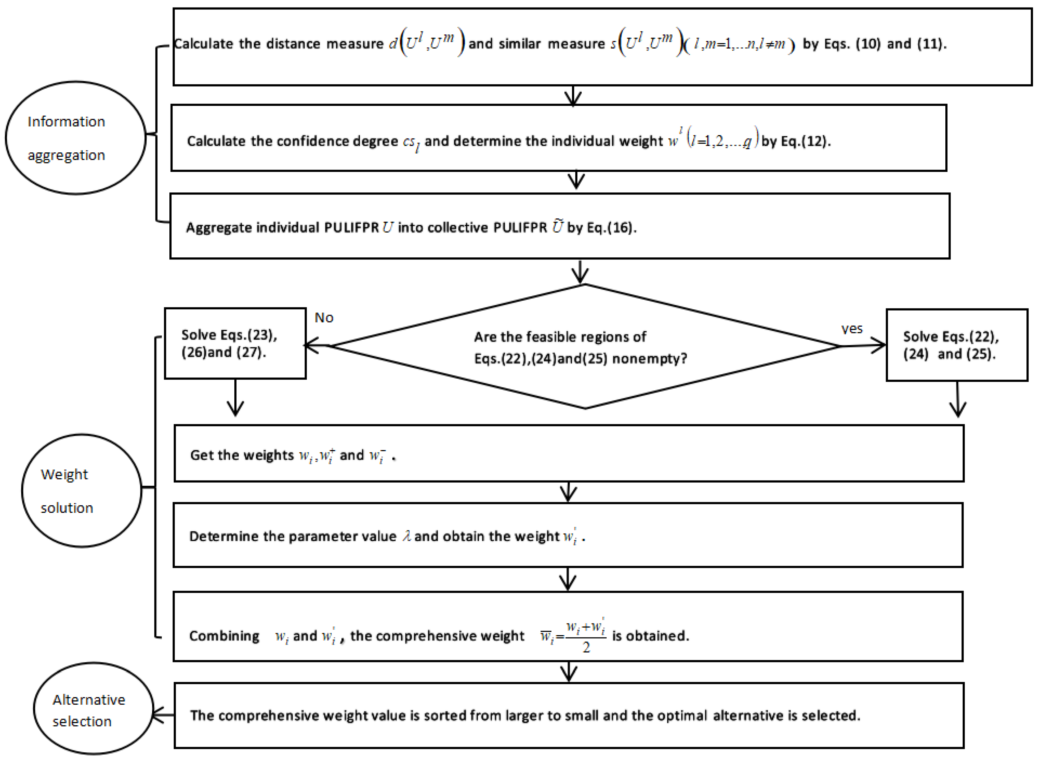
Summarizing above analyses, a new method for GDM with PULIFPR is developed as follows:

Step 1. Calculate the distance measure $d(U^l,U^m)$ and similar measure $s(U^l,U^m)(l,m=1,2,\cdots ,q,l\ne m)$ between individual PULIFPRs by Equations (10) and (11).

Step 2. Use Equation (12) to calculate the confidence degree $c{s}_l$ and determine the individual weight $w^l(l=1,2,\cdots ,q)$.

Step 3. Aggregating individual PULIFPR U into collective PULIFPR $\tilde{U}$ by Equation (16).

Step 4. When feasible regions of Models (22), (24) and (25) are nonempty, priority weights $w_i,w_i^{+}$ and $w_i^{-}$ can be solved respectively. Otherwise, priority weights $w_i,w_i^{+}$ and $w_i^{-}$ shall be obtained by solving Equations (23), (26) and (27).

Step 5. Determining the risk parameter value $\lambda$, and then the compromise weight $w_i^{\prime }$ is obtained by Equation (28).

Step 6. Combining $w_i$ and $w_i^{\prime }$, the comprehensive weight $\overline{w_i}=\frac{w_i+w_i^{\prime }}{2}$ is obtained.

Step 7. According to the comprehensive weight value to compare the alternatives, the best alternative has the bigger value.

The graphical process of solving GDM using PULIFPR is shown in Figure 2.

5. Case Application and Comparative Analysis

In order to demonstrate the effectiveness and practicability of the proposed method, this section is mainly divided into two parts. The first part discusses the application of the proposed method in the world VR industry conference 2018. The second part gives the comparative analysis between the proposed method and other methods.

5.1. Application in VR Project Selection

In recent years, virtual reality (VR) technology has received unprecedented attention from all sectors of society, and it is regarded as the portal of the next generation general computing platform and Internet along with augmented reality (AR) and mixed reality (MR). In addition, as an important force leading a new round of industrial reform in the world, it plays an important role in promoting new economic development. Therefore, in order to explore the key and common problems in the development of VR, as well as the industrial development trend and solutions, the 2018 world VR industry conference was successfully held in nanchang, jiangxi province on 19 October. As one of the important activities of the conference, the industrial counterpart conference was successfully held in nanchang on 20 October.

However, in order to ensure the successful holding of the industrial docking conference, it is particularly important for the organizers to have extensive and in-depth communication with the investors in the early stage of the conference. On the one hand, it can enable investors to have a deep and sufficient understanding of each VR project in our province so that investors can select the best cooperation project. On the other hand, it is convenient for every VR industry company in our province to select the best partner or investor. Finally, the cooperation agreements reached at the industry conference are guaranteed. Therefore, the communication and mutual selection process is an important preparation work in the early stage of the conference.

Due to the complexity of VR technology, VR project selection is a very challenging task for investors. It requires investors to make a comprehensive analysis and judgment on the competitive advantage, profitability, viability and development potential of VR project from the perspectives of simulation technology and computer graphics, man-machine interface technology, sensor technology and network technology, etc. Therefore, the project selection process is often a GDM. Without loss of generality, in order to demonstrate the GDM process using the proposed method, we take the four important projects selected by Microsoft as an example. The four projects are Touch display integration project $x_1$, Optoelectronic project $x_2$, Network security industry center project $x_3$ and Intelligent VR visual equipment project $x_4$ respectively.

In view of the complexity of VR project, Microsoft sent two investment teams ($e_1,e_2$) to inspect the project content and one technical team ($e_3$) to inspect the company’s technical equipment. Due to the wide range of knowledge involved in VR project and the complexity of factors to be considered by DMs, the decision team can only give judgment information from positive and negative aspects based on the LTS S = {$s_0$: extremely poor, $s_1$: very poor, $s_2$: poor, $s_3$: slightly poor, $s_4$: fair, $s_5$: slightly good, $s_6$: good, $s_7$: very good, $s_8$: extremely good}.

For example, by analyzing and comparing projects $x_1$ and $x_2$, the decision team $e_1$ gave the following judgment information:

$$u{(p)}_{12}=\{\langle ([s_4,s_6],[s_1,s_1]),0.45\rangle ,\langle ([s_3,s_5],[s_1,s_2]),0.5\rangle \}$$

where $[s_4,s_6]$ indicates that the DM’s preference degree for $x_1$ over $x_2$ is between fair and good, $[s_1,s_1]$ expresses that the DM’s non-preference degree for $x_1$ over $x_2$ is very poor. The probability 0.45 indicates that 45% of the people in investment teams $e_1$ give interval intuitionistic judgment information $([s_4,s_6],[s_1,s_1])$. Similarly, PULIFE $\langle ([s_3,s_5],[s_1,s_2]),0.5\rangle$ indicated that 50% of the people in investment team $e_1$ gave the interval intuitionistic judgment information as $([s_3,s_5],[s_1,s_2])$. In addition, 5% of the people failed to give any judgment information.

Now, we regard the three teams $e_1,e_2$ and $e_3$ sent by Microsoft as three individuals, and take the four projects of jiangxi province, $x_1,x_2,x_3$, and $x_4$ as the alternatives. The preference information given by the three teams in the form of PULIFPR is as follows

$U_1={(u_1{(p)}_{ij})}_{4\times 4},(i,j=1,2,3,4)$

where

$$\begin{array}{cc}\hfill u_1{(p)}_{11}& =u_1{(p)}_{22}=u_1{(p)}_{33}=u_1{(p)}_{44}=s_4;\hfill \\ \hfill u_1{(p)}_{12}& =\{\langle ([s_1,s_3],[s_4,s_5]),0.3\rangle ,\langle ([s_1,s_2],[s_5,s_6]),0.6\rangle \}\hfill \\ \hfill u_1{(p)}_{13}& =\{\langle ([s_4,s_6],[s_0,s_1]),0.8\rangle ,\langle ([s_5,s_6],[s_1,s_2]),0.2\rangle \}\hfill \\ \hfill u_1{(p)}_{14}& =\{\langle ([s_3,s_4],[s_4,s_4]),0.6\rangle ,\langle ([s_2,s_3],[s_4,s_5]),0.2\rangle \}\hfill \\ \hfill u_1{(p)}_{23}& =\{\langle ([s_0,s_2],[s_6,s_6]),0.7\rangle ,\langle ([s_1,s_3],[s_5,s_5]),0.3\rangle \}\hfill \\ \hfill u_1{(p)}_{24}& =\{\langle ([s_5,s_6],[s_0,s_1]),0.2\rangle ,\langle ([s_6,s_7],[s_0,s_1]),0.8\rangle \}\hfill \\ \hfill u_1{(p)}_{34}& =\{\langle ([s_0,s_1],[s_5,s_6]),0.9\rangle ,\langle ([s_0,s_1],[s_7,s_7]),0.1\rangle \}\hfill \end{array}$$

$U_2={(u_2{(p)}_{ij})}_{4\times 4},(i,j=1,2,3,4)$

where

$$\begin{array}{cc}\hfill u_2{(p)}_{11}& =u_2{(p)}_{22}=u_2{(p)}_{33}=u_2{(p)}_{44}=s_4;\hfill \\ \hfill u_2{(p)}_{12}& =\{\langle ([s_2,s_3],[s_4,s_4]),0.4\rangle ,\langle ([s_3,s_4],[s_4,s_5]),0.6\rangle \}\hfill \\ \hfill u_2{(p)}_{13}& =\{\langle ([s_1,s_2],[s_5,s_5]),0.3\rangle ,\langle ([s_2,s_3],[s_4,s_5]),0.5\rangle \}\hfill \\ \hfill u_2{(p)}_{14}& =\{\langle ([s_5,s_6],[s_1,s_1]),0.3\rangle ,\langle ([s_6,s_6],[s_1,s_2]),0.6\rangle \}\hfill \\ \hfill u_2{(p)}_{23}& =\{\langle ([s_6,s_7],[s_1,s_1]),0.4\rangle ,\langle ([s_5,s_6],[s_1,s_2]),0.5\rangle \}\hfill \\ \hfill u_2{(p)}_{24}& =\{\langle ([s_0,s_2],[s_5,s_6]),0.7\rangle ,\langle ([s_1,s_2],[s_6,s_6]),0.3\rangle \}\hfill \\ \hfill u_2{(p)}_{34}& =\{\langle ([s_3,s_5],[s_2,s_2]),0.4\rangle ,\langle ([s_2,s_5],[s_1,s_2]),0.4\rangle \}\hfill \end{array}$$

$U_3={(u_3{(p)}_{ij})}_{4\times 4},(i,j=1,2,3,4)$

where

$$\begin{array}{cc}\hfill u_3{(p)}_{11}& =u_1{(p)}_{22}=u_1{(p)}_{33}=u_1{(p)}_{44}=s_4;\hfill \\ \hfill u_3{(p)}_{12}& =\{\langle ([s_2,s_4],[s_3,s_4]),0.2\rangle ,\langle ([s_4,s_5],[s_3,s_3]),0.5\rangle \}\hfill \\ \hfill u_3{(p)}_{13}& =\{\langle ([s_1,s_2],[s_5,s_6]),0.8\rangle ,\langle ([s_2,s_3],[s_5,s_5]),0.2\rangle \}\hfill \\ \hfill u_3{(p)}_{14}& =\{\langle ([s_7,s_8],[s_0,s_0]),0.3\rangle ,\langle ([s_6,s_7],[s_1,s_1]),0.6\rangle \}\hfill \\ \hfill u_3{(p)}_{23}& =\{\langle ([s_0,s_1],[s_6,s_6]),0.6\rangle ,\langle ([s_1,s_1],[s_6,s_7]),0.3\rangle \}\hfill \\ \hfill u_3{(p)}_{24}& =\{\langle ([s_4,s_5],[s_1,s_2]),0.7\rangle ,\langle ([s_5,s_5],[s_2,s_3]),0.3\rangle \}\hfill \\ \hfill u_3{(p)}_{34}& =\{\langle ([s_7,s_7],[s_0,s_1]),0.3\rangle ,\langle ([s_5,s_6],[s_1,s_2]),0.6\rangle \}\hfill \end{array}$$

Since the upper triangle of PULIFPR has a one-to-one correspondence with the lower triangle, we only give the upper triangle of the preference relation. According to Section 4.3, we can solve the GDM problem about project selection as follows:

Step 1: According to Equation (10), the distance measure between $U_1$ and $U_2$ is $d(U_1,U_2)=\frac{1}{4\times 3}(|f_{12}^1-f_{12}^2|+|g_{12}^1-g_{12}^2|+|f_{13}^1-f_{13}^2|+|g_{13}^1-g_{13}^2|+|f_{14}^1-f_{14}^2|+|g_{14}^1-g_{14}^2|+|f_{23}^1-f_{23}^2|+|g_{23}^1-g_{23}^2|+|f_{24}^1-f_{24}^2|+|g_{24}^1-g_{24}^2|+|f_{34}^1-f_{34}^2|+|g_{34}^1-g_{34}^2|)=\frac{1}{12}(|0.2531-0.425|+|0.775-0.2719|+|0.3563-0.7031|+|0.225-0.7125|+|0.8625-0.2188|+|0.1781-0.5|+|0.1313-0.075|+|0.275-0.1188|+|0.0625-0.0938|+|0.125-0.0875|+|0.15-0.15|+|0.2313-0.25|)=0.2313$, Similarly, we can calculate $d(U_1,U_3)=0.1930$ and $d(U_2,U_3)=0.1398$ respectively, so the corresponding similarity degree is $s(U_1,U_2)=0.7687,s(U_1,U_3)=0.8070$ and $s(U_2,U_3)=0.8602$ respectively.

Step 2: According to Equation (12), the confidence degree of the three teams can be calculated as $c{s}_1=s(U_1,U_2)+s(U_1,U_3)=1.5758,c{s}_2=1.6289$ and $c{s}_3=1.6672$, so the weight of each team can be further determined as $w^1=\frac{c{s}_1}{c{s}_1+c{s}_2+c{s}_3}=0.3234,w^2=0.3344$, and $w^3=0.3422$.

Step 3: By using Equation (16), the collective PULIFPR $\tilde{U}$ can be obtained as follows

$\tilde{U}={(\tilde{u}{(p)}_{ij})}_{4\times 4},(i,j=1,2,3,4)$

where

$$\begin{array}{cc}\hfill \tilde{u}{(p)}_{11}& =\tilde{u}{(p)}_{22}=\tilde{u}{(p)}_{33}=\tilde{u}{(p)}_{44}=s_4;\hfill \\ \hfill \tilde{u}{(p)}_{12}& =\{\langle ([s_{1.6766},s_{3.3442}],[s_{3.6578},s_{4.3234}]),0.3\rangle ,\langle ([s_{2.6953},s_{3.6953}],[s_{3.0717},s_{4.6390}]),0.5667\rangle \};\hfill \\ \hfill \tilde{u}{(p)}_{13}& =\{\langle ([s_{1.9703},s_{3.2938}],[s_{3.3828},s_{4.0484}]),0.6333\rangle ,\langle ([s_{2.9703},s_{3.9703}],[s_{3.3719},s_{4.0297}]),0.3\rangle \};\hfill \\ \hfill \tilde{u}{(p)}_{14}& =\{\langle ([s_{5.0375},s_{6.0375}],[s_{1.6281},s_{1.6281}]),0.4\rangle ,\langle ([s_{4.7062},s_{5.3719}],[s_{1.9703},s_{2.6281}]),0.4667\rangle \};\hfill \\ \hfill \tilde{u}{(p)}_{23}& =\{\langle ([s_{2.0061},s_{3.3295}],[s_{4.3283},s_{4.3283}]),0.5667\rangle ,\langle ([s_{2.3374},s_{3.3186}],[s_{4.0048},s_{4.6814}]),0.3667\rangle \};\hfill \\ \hfill \tilde{u}{(p)}_{24}& =\{\langle ([s_{2.9860},s_{4.3204}],[s_{2.0140},s_{3.0140}]),0.5333\rangle ,\langle ([s_{3.9860},s_{4.6438}],[s_{2.6905},s_{3.3562}]),0.4667\rangle \};\hfill \\ \hfill \tilde{u}{(p)}_{34}& =\{\langle ([s_{3.3985},s_{4.3906}],[s_{2.2859},s_{2.9516}]),0.5333\rangle ,\langle ([s_{2.3797},s_{4.0484}],[s_{2.9407},s_{3.6172}]),0.3667\rangle \}.\hfill \end{array}$$

Step 4: The non-fuzzy uncertain information values $f_{ij}(i,j=1,2,3,4,i<j)$ and the fuzzy uncertain information values $g_{ij}(i,j=1,2,3,4,i<j)$ of PULIFPR $\tilde{U}$ are calculated respectively. By substituting them into Equation (22), the following model can be obtained

$$\max \theta ={\theta }_{12}+{\theta }_{13}+{\theta }_{14}+{\theta }_{23}+{\theta }_{24}+{\theta }_{34}$$

$$s.t.\left\{\begin{array}{c}[0.3822{\theta }_{12}+0.1235(1-{\theta }_{12})](w_1+w_2)-w_1=0,\hfill \\ {\theta }_{13}+0.1619(1-{\theta }_{13})](w_1+w_3)-w_1=0,\hfill \\ {\theta }_{14}+0.0803(1-{\theta }_{14})](w_1+w_4)-w_1=0,\hfill \\ {\theta }_{23}+0.1091(1-{\theta }_{23})](w_2+w_3)-w_2=0,\hfill \\ {\theta }_{24}+0.1608(1-{\theta }_{24})](w_2+w_4)-w_2=0,\hfill \\ {\theta }_{34}+0.1682(1-{\theta }_{34})](w_3+w_4)-w_3=0,\hfill \\ w_1+w_2+w_3>w_4-0.5,w_1+w_2+w_4>w_3-0.5,\hfill \\ w_1+w_3+w_4>w_2-0.5,w_2+w_3+w_4>w_1-0.5,\hfill \\ w_1+w_2+w_3+w_4=1,w_1,w_2,w_3,w_4\ge 0,\hfill \\ 0\le {\theta }_{12},{\theta }_{13},{\theta }_{14},{\theta }_{23},{\theta }_{24},{\theta }_{34}\le 1.\hfill \end{array}\right.$$

(29)

By solving this model, priority weights and parameter values can be obtained as $w_1=0.1227,w_2=0.1984,w_3=0.3333,w_4=0.3456,{\theta }_{13}=0.4162,{\theta }_{14}=0.3425,{\theta }_{24}=0.4916,{\theta }_{12}={\theta }_{23}={\theta }_{34}=1$.

Step 5: By calculating the optimistic judgment values $a_{ij}={\sum }_{k=1}^{\#u(p)}{p}^k\times \frac{I(s_{{\overline{u}}_{ij}^k})-I(s_{{\underline{v}}_{ij}^k})+2\tau }{4\tau }$ and pessimistic judgment values $b_{ij}={\sum }_{k=1}^{\#u(p)}{p}^k\times \frac{I(s_{{\underline{u}}_{ij}^k})-I(s_{{\overline{v}}_{ij}^k})+2\tau }{4\tau },(i,j=1,2,3,4,i<j)$ and substituting them into Equations (24) and (25) respectively to solve the weight. But their feasible regions are all empty. Therefore, substitute the values of $a_{ij}$ and $b_{ij}$ into Equations (26) and (27) respectively, then the priority weights can be obtained as follows

$w_1^{+}=0.2149,w_2^{+}=0.2631,w_3^{+}=0.3700,w_4^{+}=0.1520,$.

$w_1^{-}=0.1395,w_2^{-}=0.3034,w_3^{-}=0.2432,w_4^{-}=0.3139$.

Without loss of generality, assume that the value of risk parameter $\lambda$ determined by Microsoft is 0.5. Then the priority weights can be obtained as $w_1^{\prime }=0.5w_1^{+}+(1-0.5)w_1^{-}=0.1783,w_2^{\prime }=0.2823,w_3^{\prime }=0.3058,w_4^{\prime }=0.2336$.

Step 6: Combining the results obtained in steps 4 and 5, the comprehensive ranking weight of $\tilde{U}$ can be obtained as $\overline{w_1}=0.1505,\overline{w_2}=0.2404,\overline{w_3}=0.3195,\overline{w_4}=0.2896$. Therefore, the final ranking result is $\overline{w_3}>\overline{w_4}>\overline{w_2}>\overline{w_1}$, namely, $x_3$ is the best candidate partner of Microsoft.

In addition, the sorting results for different risk parameter values $\lambda$ are shown in

Table 2. Ranking orders of alternatives with different parameter values $\lambda$.

$\mathit{\lambda }$	$\overline{{\mathit{w}}_1}$	$\overline{{\mathit{w}}_2}$	$\overline{{\mathit{w}}_3}$	$\overline{{\mathit{w}}_4}$	Ranking Order
0.1	0.1350	0.2488	0.2945	0.3217	$x_4>x_3>x_2>x_1$
0.2	0.1388	0.2467	0.3008	0.3137	$x_4>x_3>x_2>x_1$
0.3	0.1427	0.2446	0.3070	0.3057	$x_3>x_4>x_2>x_1$
0.4	0.1466	0.2425	0.3133	0.2976	$x_3>x_4>x_2>x_1$
0.5	0.1505	0.2404	0.3195	0.2896	$x_3>x_4>x_2>x_1$
0.6	0.1544	0.2382	0.3258	0.2816	$x_3>x_4>x_2>x_1$
0.7	0.1583	0.2361	0.3321	0.2735	$x_3>x_4>x_2>x_1$
0.8	0.1622	0.2340	0.3383	0.2655	$x_3>x_4>x_2>x_1$
0.9	0.1660	0.2319	0.3446	0.2575	$x_3>x_4>x_2>x_1$

.

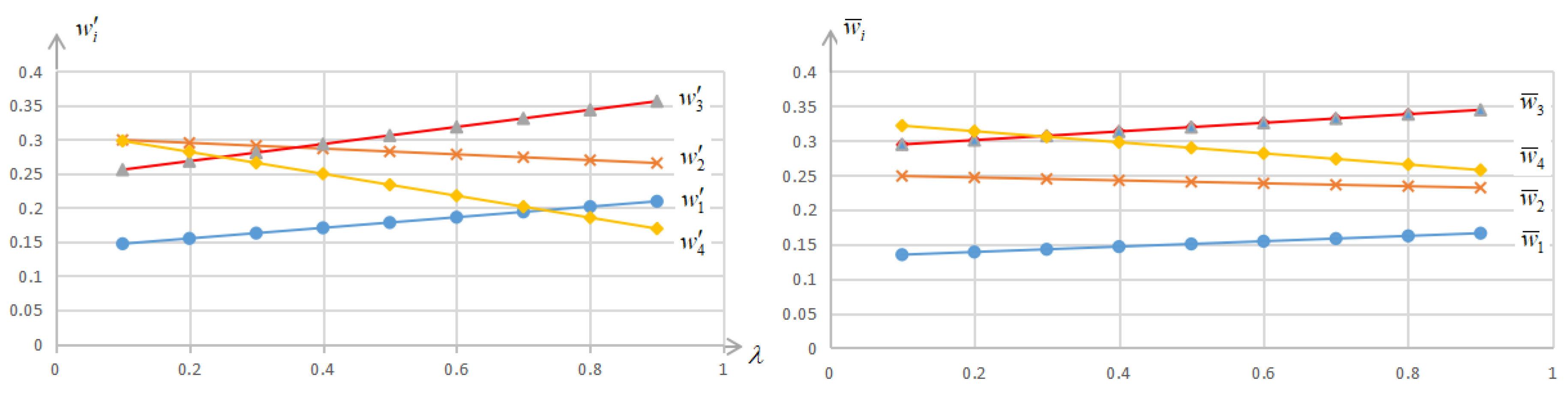
It can be seen from Table 2 that different sorting results may occur for different risk parameter values $\lambda$. When $0<\lambda <0.3$, the sorting result is $x_4>x_3>x_2>x_1$, and when $0.3\le \lambda \le 0.9$, the sorting result is $x_3>x_4>x_2>x_1$. This fully demonstrates the importance of DM’s risk attitude in GDM and the rationality of the method proposed in this paper. In addition, to further reflect the impact of risk parameter value $\lambda$ on GDM. We give the variation trend diagram of the compromise weight $w_i^{\prime }$ and the comprehensive weight $\overline{w}$ (see Figure 3).

It can be seen intuitively from Figure 3 that the variation trend of the compromise weight $w_i^{\prime }$ and the comprehensive weight $\overline{w_i}$ with the increase of $\lambda$. Furthermore, by comparing $w_i^{\prime }$ and $\overline{w_i}$, it is easy to see that project $x_4$ is greatly influenced by $\lambda$ when only taking into account DM’s risk attitude (as the value of $\lambda$ increases, the value of $w_4^{\prime }$ decreases from the maximum to the minimum), while its comprehensive weight $\overline{w_4}$ is less affected by $\lambda$. This further illustrates the necessity and rationality of comprehensive consideration of risk attitude, fuzzy and non-fuzzy uncertain information in GDM problems.

5.2. Comparison Analyses

As a new preference relation, PULIFPR expands the application scope of qualitative information in fuzzy theory and improves the applicability of linguistic terms in GDM. Moreover, as an extension form of LPR, it can be transformed into various LPRs through corresponding changes. Therefore, the method proposed in this paper is also applicable to other types of preference relations, and its specific advantages compared with existing series methods are shown in

Table 3. Comparison of different methods.

Methods	Preference Relations	Considering the Non-Preference Information	Considering the Probability Distribution	Considering the Fuzzy Uncertainty (Ignorance Information)	Determining the Individual Weight	Avoiding Consistency Checks and Corrections	Considering the Risk Attitudes of DMs
The proposed method	PULIFPRs	Yes	Yes	Yes	Yes	Yes	Yes
Meng et al.’s method [27]	LIFPRs	Yes	No	No	No	No	No
Xie et al.’s method [37]	PULPRs	No	Yes	No	No	No	No
Zhang et al.’s method [38]	PLPRs	No	Yes	No	No	No	No
Wan et al.’s method [36]	IVIFPRs	Yes	No	Yes	Yes	No	Yes
Liao et al.’s method [39]	IFPRs	Yes	No	No	No	No	No
Wan et al.’s method [32]	IVFPRs	No	No	No	Yes	No	Yes
Zhao et al.’s method [40]	LPRs	No	No	Yes	Yes	No	No
Meng et al.’s method [31]	IVIFPRs	Yes	No	No	Yes	No	No

.

It is easy to see from Table 3 that compared with other methods, the methods proposed in this paper have many advantages, which not only make up for the deficiencies of current methods, but also avoid the detection and correction of consistency in GDM problems. Specifically speaking, compared with the model proposed by the existing methods, the specific advantages of the model proposed in this paper are as follows

(1)

Compared with models M-1 and M-3 in method [27], the model proposed in this paper can directly obtain the priority weight of preference relation without consistency test and correction.

(2)

Compared with Algorithms 1 and 2 in method [37], the algorithm proposed in this paper provides a method to determine the individual weight, and the consensus collective preference relation can be obtained directly without iterative calculation.

(3)

Compared with the model proposed by wan et al. [36], the model proposed in this paper considers the probability distribution of uncertain information, which is more suitable for large-scale GDM problems in complex environments and can ensure the consistency of collective preference relations.

(4)

Compared with the GPM proposed by liao et al. [39], the model proposed in this paper considers both the risk attitude of DMs and the information that they fail to grasp, which improves the rationality and accuracy of decision-making results.

In addition, PULIFS proposed in this paper is a comprehensive extension of the LTS, which can be converted into other sets according to the practical needs of decision problems. Therefore, PULIFS is more general and representative than many existing fuzzy sets, and it is more flexible in the application of decision problem. Furthermore, we classify the information expressed by PULIFPR as fuzzy and non-fuzzy uncertain information to fully consider the preferences, non-preferences and unknown information of the decision-maker. Thus, the method proposed in this paper comprehensively reflects the subjective hesitation, uncertainty and objective randomness existing in actual decision-making problems, and thus ensures the rationality of the DM results.

To sum up, the advantages of the proposed method in practical application can be summarized as follows

(1)

Compared with the general preference relation, the PULIFPR proposed in this paper can express both individual preference and group preference, which is more suitable for the increasingly complex decision-making environment. Therefore, the decision-making method proposed in this paper has a broad application prospect. Such as the selection of investment projects, the formulation of enterprise marketing plans, the introduction of talents in institutions, etc.

(2)

The method proposed in this paper comprehensively considers the risk attitude and fuzzy uncertain information of DMs, which is more in line with the actual decision-making situation and is easily accepted and adopted by DMs.

(3)

The proposed model can guarantee the consistency of the collective preference relation without checking and revising, so it is more simple and accurate in practical application.

However, although the method proposed in this paper has many advantages, it also has some limitations. On the one hand, this paper considers the risk attitude of decision makers, but fails to give a method to determine the value of risk parameters; on the other hand, this paper does not consider the group decision-making problem in the context of incomplete information. Therefore, the method of determining the risk parameter value and extending the proposed method to an incomplete environment will be the future research direction.

6. Conclusions

This paper first briefly summarizes the development history of LTS and puts forward PULIFS, which extends the application of LT in fuzzy theory and promotes the application of qualitative information in GDM. Secondly, the definition of PULIFPR is proposed, which can fully express the subjective hesitation of the decision-maker in the DM problem as well as the uncertainty and randomness of the objective existence. We then defined the distance measure between PULIFSs and used it to determine the individual objective weight, thus increasing the accuracy of information aggregation. Subsequently, a series of GPMs for solving priority weights were established, which not only fully considered the fuzziness of information and DM’s risk attitude, but also avoided the test and correction of consistency in GDM. Moreover, we take the project selection of world VR industry conference 2018 as an example demonstrates the effectiveness and practicality of the proposed method.

It is worth noting that this paper only discusses the application of qualitative information in GDM, so it will be an interesting research direction to apply the method proposed in this paper to the quantitative decision-making field, such as IVIFS [41] or PIVIHFS [28], and the decision problem in heterogeneous environment (both qualitative and quantitative information should be considered). In addition, since this paper studies the uncertain problem in a complex environment, it will be a worthy research direction to combine the proposed method with the complex network with fuzzy logic units [42].

References

- Zadeh, L.A. The concept of a linguistic variable and its application to approximate reasoning—I. Inf. Sci. 1975, 8, 199–249. [Google Scholar] [CrossRef]
- Zadeh, L.A. The concept of a linguistic variable and its application to approximate reasoning—II. Inf. Sci. 1975, 8, 301–357. [Google Scholar] [CrossRef]
- Zadeh, L.A. The concept of a linguistic variable and its application to approximate reasoning—III. Inf. Sci. 1975, 9, 43–80. [Google Scholar] [CrossRef]
- Yager, R.R. A new methodology for ordinal multiobjective decisions based on fuzzy sets. Decis. Sci. 1981, 12, 589–600. [Google Scholar] [CrossRef]
- Degadni, R.; Bortolan, G. The problem of linguistic approximation in clinical decision making. Int. J. Approx. Reason. 1988, 2, 143–162. [Google Scholar] [CrossRef]
- Delgado, M.; Verdegay, J.L.; Vila, M.A. On aggregation operations of linguistic labels. Int. J. Intell. Syst. 1993, 8, 351–370. [Google Scholar] [CrossRef]
- Herrera, F.; Martinez, L. A 2-tuple fuzzy linguistic representation model for computing with words. IEEE Trans. Fuzzy Syst. 2000, 8, 746–752. [Google Scholar]
- Xu, Z.S. A method based on linguistic aggregation operators for group decision making with linguistic preference relations. Inf. Sci. 2004, 166, 19–30. [Google Scholar] [CrossRef]
- Xu, Z.S. Uncertain linguistic aggregation operators based approach to multiple attribute group decision making under uncertain linguistic environment. Inf. Sci. 2004, 168, 171–184. [Google Scholar] [CrossRef]
- Rodriguez, R.M.; Martinez, L.; Herrera, F. Hesitant Fuzzy Linguistic Term Sets for Decision Making. IEEE Trans. Fuzzy Syst. 2012, 20, 109–119. [Google Scholar] [CrossRef]
- Meng, F.; Chen, X.; Zhang, Q. Multi-attribute decision analysis under a linguistic hesitant fuzzy environment. Inf. Sci. 2014, 267, 287–305. [Google Scholar] [CrossRef]
- Zhang, H.M. Linguistic Intuitionistic Fuzzy Sets and Application in MAGDM. J. Appl. Math. 2014, 1–11. [Google Scholar] [CrossRef]
- Ye, J. An extended TOPSIS method for multiple attribute group decision making based on single valued neutrosophic linguistic numbers. J. Intell. Fuzzy Syst. 2015, 28, 247–255. [Google Scholar]
- Pang, Q.; Wang, H.; Xu, Z.S. Probabilistic linguistic term sets in multi-attribute group decision making. Inf. Sci. 2016, 369, 128–143. [Google Scholar] [CrossRef]
- Lin, M.W.; Xu, Z.S.; Zhai, Y.L.; Yao, Z.Q. Multi-attribute group decision-making under probabilistic uncertain linguistic environment. J. Oper. Res. Soc. 2017, 22, 1–15. [Google Scholar] [CrossRef]
- Bai, C.; Zhang, R.; Shen, S.; Huang, C.; Fan, X. Interval valued probabilistic linguistic term sets in multi-criteria group decision making. Int. J. Intell. Syst. 2018, 33, 1301–1321. [Google Scholar] [CrossRef]
- Zhang, R.C.; Li, Z.M.; Liao, H.C. Multiple-attribute decision-making method based on the correlation coefficient between dual hesitant fuzzy linguistic term sets. Knowl.-Based Syst. 2018, 159, 186–192. [Google Scholar] [CrossRef]
- Pamucar, D.; Badi, I.; Sanja, K.; Obradovic, R. A Novel Approach for the Selection of Power-Generation Technology Using a Linguistic Neutrosophic CODAS Method: A Case Study in Libya. Energies 2018, 11, 2489. [Google Scholar] [CrossRef]
- Liu, F.; Aiwu, G.; Lukovac, V.; Vukic, M. A multicriteria model for the selection of the transport service provider: A single valued neutrosophic DEMATEL multicriteria model. Decision Mak. Appl. Manag. Eng. 2018, 1, 121–130. [Google Scholar] [CrossRef]
- Orlorski, S.A. Decision making with a fuzzy preference relation. Fuzzy Sets Syst. 1978, 3, 155–167. [Google Scholar]
- Saaty, T.L. The Analytical Hierarchy Process; McGraw-Hill: New York, NY, USA, 1980. [Google Scholar]
- Herrera, F.; Herrera-Viedma, E.; Verdegay, J.L. A model of consensus in group decision making under linguistic assessments. Fuzzy Sets Syst. 1996, 78, 73–87. [Google Scholar] [CrossRef]
- Xu, Z.S. On compatibility of interval fuzzy preference relations. Fuzzy Optim. Decis. Mak. 2004, 3, 217–225. [Google Scholar] [CrossRef]
- Saaty, T.L.; Vargas, L.G. Uncertainty and rank order in the analytic hierarchy process. Eur. J. Oper. Res. 1987, 32, 107–117. [Google Scholar] [CrossRef]
- Xu, Z.S. Intuitionistic preference relations and their apllication in group decision making. Inf. Sci. 2007, 177, 2363–2379. [Google Scholar] [CrossRef]
- Xia, M.M.; Xu, Z.S.; Liao, H.C. Preference relations based on intuitionistic multiplicative information. IEEE Trans. Fuzzy Syst. 2013, 21, 113–133. [Google Scholar]
- Meng, F.Y.; Tang, J.; Fujita, H. Linguistic intuitionistic fuzzy preference relations and their application to multi-criteria decision making. Inf. Fusion 2019, 46, 77–90. [Google Scholar] [CrossRef]
- Zhai, Y.L.; Xu, Z.S.; Liao, H.C. Measures of Probabilistic Interval-Valued Intuitionistic Hesitant Fuzzy Sets and the Application in Reducing Excessive Medical Examinations. IEEE Trans. Fuzzy Syst. 2018, 26, 1651–1670. [Google Scholar] [CrossRef]
- Tanino, T. Fuzzy preference orderings in group decision making. Fuzzy Sets Syst. 1984, 12, 117–131. [Google Scholar] [CrossRef]
- Chiclana, F.; Herrera-Viedma, E.; Alonso, S.; Herrera, F. Cardinal consistency of reciprocal preference relations: A characterization of mulitiplicative transitivity. IEEE Trans. Fuzzy Syst. 2009, 17, 14–23. [Google Scholar] [CrossRef]
- Meng, F.Y.; Tang, J.; Wang, P.; Chen, X.H. A programming-based algorithm for interval-valued intuitionistic fuzzy group decision making. Knowl.-Based Syst. 2018, 144, 122–143. [Google Scholar] [CrossRef]
- Wan, S.P.; Wang, F.; Dong, J.Y. A group decision making method with interval valued fuzzy preference relations based on the geometric consistency. Inf. Fusion 2018, 40, 87–100. [Google Scholar] [CrossRef]
- Wu, J.; Chiclana, F.; Liao, H.C. Isomorphic Multiplicative Transitivity for Intuitionistic and Interval-Valued Fuzzy Preference Relations and Its Application in Deriving Their Priority Vectors. IEEE Trans. Fuzzy Syst. 2018, 26, 193–202. [Google Scholar] [CrossRef]
- Zhou, W.; Xu, Z.S. Probability Calculation and Element Optimization of Probabilistic Hesitant Fuzzy Preference Relations Based on Expected Consistency. IEEE Trans. Fuzzy Syst. 2018, 26, 1367–1378. [Google Scholar] [CrossRef]
- Wang, Z.J. A Goal Programming Based Heuristic Approach to Deriving Fuzzy Weights in Analytic Form from Triangular Fuzzy Preference Relations. IEEE Trans. Fuzzy Syst. 2018. [Google Scholar] [CrossRef]
- Wan, S.P.; Wang, F.; Dong, J.Y. Three-Phase Method for Group Decision Making With Interval-Valued Intuitionistic Fuzzy Preference Relations. IEEE Trans. Fuzzy Syst. 2018, 26, 998–1010. [Google Scholar] [CrossRef]
- Xie, W.Y.; Ren, Z.L.; Xu, Z.S.; Wang, H. The consensus of probabilistic uncertain linguistic preference relations and the application on the virtual reality industry. Knowl.-Based Syst. 2018, 162, 14–28. [Google Scholar] [CrossRef]
- Zhang, Y.X.; Xu, Z.S.; Liao, H.C. A consensus process for group decision making with probabilistic linguistic preference relations. Inf. Sci. 2017, 414, 260–275. [Google Scholar] [CrossRef]
- Liao, H.C.; Xu, Z.; Zeng, X.J.; Merigó, J.M. Framework of group decision making with intuitionistic fuzzy preference information. IEEE Trans. Fuzzy Syst. 2015, 23, 1211–1227. [Google Scholar] [CrossRef]
- Zhao, M.; Ma, X.Y.; Wei, D.W. A method considering and adjusting individual consistency and group consensus for group decision making with incomplete linguistic preference relations. Appl. Soft Comput. 2017, 54, 322–346. [Google Scholar] [CrossRef]
- Atanassov, K.; Gargov, G. Interval valued intuitionistic fuzzy sets. Fuzzy Sets Syst. 1989, 31, 343–349. [Google Scholar] [CrossRef]
- Bucolo, M.; Fortuna, L.; La Rosa, M. Complex dynamics through fuzzy chains. IEEE Trans. Fuzzy Syst. 2004, 12, 289–295. [Google Scholar] [CrossRef]
Figure 1.
The uncertainty space of probabilistic uncertain linguistic intuitionistic fuzzy preference relation (PULIFPR).
Figure 2.
Process of group decision-making (GDM) with PULIFPRs.
Figure 3.
The variation trend of weights and based on different parameter values .