An Investigation on the Prime and Twin Prime Number Functions by Periodical Binary Sequences and Symmetrical Runs in a Modified Sieve Procedure

Abstract

In this work, the Sieve of Eratosthenes procedure (in the following named Sieve procedure) is approached by a novel point of view, which is able to give a justification of the Prime Number Theorem (P.N.T.). Moreover, an extension of this procedure to the case of twin primes is formulated. The proposed investigation, which is named Limited INtervals into PEriodical Sequences (LINPES) relies on a set of binary periodical sequences that are evaluated in limited intervals of the prime characteristic function. These sequences are built by considering the ensemble of deleted (that is, 0) and undeleted (that is, 1) integers in a modified version of the Sieve procedure, in such a way a symmetric succession of runs of zeroes is found in correspondence of the gaps between the undeleted integers in each period. Such a formulation is able to estimate the prime number function in an equivalent way to the logarithmic integral function Li(x). The present analysis is then extended to the twin primes, by taking into account only the runs whose size is two. In this case, the proposed procedure gives an estimation of the twin prime function that is equivalent to the one of the logarithmic integral function ${\mathrm{Li}}_2\left(x\right)$. As a consequence, a possibility is investigated in order to count the twin primes in the same intervals found for the primes. Being that the bounds of these intervals are given by squares of primes, if such an inference were actually proved, then the twin primes could be estimated up to infinity, by strengthening the conjecture of their never-ending.

1. Introduction

The Sieve procedure is able to achieve heuristic justifications of the Prime Number Theorem (P.N.T.) [1]. Such a theorem gives the asymptotic trend of the prime number function $\pi \left(x\right)$, where $\pi \left(x\right)$ denotes the quantity of prime numbers $p$ less or equal to $x\in \mathbb{R}$, that is,

$$\pi \left(x\right)=\mathrm{number}\mathrm{of}\mathrm{primes}p,p\le x.$$

(1)

Let $\log \left(x\right)$ be the natural logarithm of $x$. If the real functions $A\left(x\right)$ and $B\left(x\right)$ are asympthotically equal, that is, $\underset{x\to \infty }{\lim }A\left(x\right)/B\left(x\right)=1$, then we say that $A\left(x\right)$ and $B\left(x\right)$ are equivalent as $x\to \infty$, and we write $A\left(x\right)\sim B\left(x\right)$. Consequently, the P.N.T. can be written as

$$\pi \left(x\right)\sim x/\log \left(x\right).$$

(2)

After the infinitude of primes was recognized since ancient times, the estimation (2) was conjectured by Gauss [2] and Legendre [3] at the end of the $18th$ century. Gauss himself improved Equation (2), by considering the logarithmic integral function Li(x), which is defined as

$$\mathrm{Li}\left(x\right)={\int }_2^x\frac{dt}{\log t}.$$

(3)

Again, the function (3) is such that

$$\pi \left(x\right)\sim \mathrm{Li}\left(x\right)$$

(4)

but the approximation (4) is much more precise than (2). In fact, it can be demonstrated that the piece $x/\log \left(x\right)$ is only the first term of the series expansion of (3). The aim of this work is to introduce a novel heuristic procedure (LINPES, Limited INtervals into PEriodical Sequences) that is equivalent to the $\mathrm{Li}\left(x\right)$ approximation, in the sense of Equation (4), apart from a simple multiplicative constant, by exploiting some binary periodic sequences, and related symmetrical runs. Pieces of these sequences compose limited intervals of the prime characteristic function ${\xi }_p\left(n\right)$, which is defined as

$${\xi }_p\left(n\right)=\left\{\begin{array}{cc}1\hfill & \mathrm{if}n\mathrm{is}\mathrm{prime}\hfill \\ 0\hfill & \mathrm{otherwise}.\hfill \end{array}\right.$$

(5)

As a matter of fact, a topic that is very much discussed nowadays in the literature just concerns the possible discovering of some regularities and periodicities in the distribution of the primes in certain intervals of the integer sequence [4]. In this work, the implications of the LINPES procedure are also investigated, in particular with an extension to the twin primes, whose distribution is given by a function known as twin prime function ${\pi }_2\left(x\right)$, which is similar to (1), that is,

$${\pi }_2\left(x\right)=\mathrm{number}\mathrm{of}\mathrm{pairs}\mathrm{of}\mathrm{twin}\mathrm{primes}(p,p+2),p\le x.$$

(6)

Unlike the case of primes, the infinitude of twin primes is still unproved. However, analogously to the P.N.T., the density of the twin primes has been conjectured [5], by considering that the probability to be a prime of an integer $n$ is equal to $1/\log \left(n\right)$. Consequently, the probability that $n$ and $n+2$ are both prime can be computed, in such a way the strong twin prime conjecture [6] gives an equivalence between the twin prime function ${\pi }_2\left(x\right)$ and the logarithmic integral function ${\mathrm{Li}}_2\left(x\right)$, that is,

$${\pi }_2\left(x\right)\sim C{\mathrm{Li}}_2\left(x\right)$$

(7)

where ${\mathrm{Li}}_2\left(x\right)$ is defined as

$${\mathrm{Li}}_2\left(x\right)={\int }_2^x\frac{dt}{{\left(\log t\right)}^2}$$

(8)

and $C=2{\mathsf{\Pi }}_2\simeq 1.3203$ is a multiplicative constant that takes into account the statistical dependence of the primes $n$ and $n+2$ [5]. The related constant ${\mathsf{\Pi }}_2\simeq 0.6602$ is named twin prime constant, that is,

$${\mathsf{\Pi }}_2=\prod _{p>2,p\mathrm{prime}}\left(1-\frac{1}{{(p-1)}^2}\right).$$

(9)

As it will be shown later, the proposed LINPES procedure is able to estimate the twin prime function in an equivalent way as the ${\mathrm{Li}}_2\left(x\right)$ function, apart from a multiplicative constant. However, this is made by admitting that a basic relation, which is true for the primes, is also valid for the twin primes. In this case, the contribution of the present work will be a more probable assertion of the infinitude of twin primes.

Before starting our discussion, we itemize the variables utilized in this paper

• $\pi \left(x\right)$: prime number function (1)
• $\mathrm{Li}\left(x\right)$: logarithmic integral function (3), which leads to an estimation of $\pi \left(x\right)$
• ${\pi }_2\left(x\right)$: twin prime number function (6)
• ${\mathrm{Li}}_2\left(x\right)$: logarithmic integral function (8), which leads to an estimation of ${\pi }_2\left(x\right)$
• $\pi \left(N\right)$: prime number function computed in the fixed integer $N$
• p: generic prime number
• $p\left(n\right)$: arithmetic function that gives the succession of primes
• ${\xi }_p\left(n\right)$: arithmetic function that gives the characteristic function of primes (5)
• $R_s\left(n\right)$: number of residual integers in the $n-th$ step of the Sieve procedure
• ${\pi }_R\left(N\right)$: estimation of $\pi \left(N\right)$ given by the heuristic method of Section 2
• $\xi (k,n)$: approximation of ${\xi }_p\left(n\right)$ after the $k-th$ step of the Sieve procedure
• $\psi (k,n)$: periodic binary sequence obtained in the $k-th$ step of the modified Sieve procedure
• $T\left(k\right)$: period of the periodic binary sequence $\psi (k,n)$
• $J(k,n)$: sliding interval whose size is the same of $I\left(k\right)$ and whose initial point is given by $n$
• $S\left(k\right)$: size of the interval $I\left(k\right)$
• $R\left(k\right)$: number of residual runs of zeroes in each period $T\left(k\right)$
• $L(m,k)$: size of the $m-th$ run of zeroes in each period $T\left(k\right)$
• $I\left(k\right)=[p{\left(k\right)}^2,p{(k+1)}^2)$: interval of ${\xi }_p\left(n\right)$ where a piece of $\psi (k,n)$ is stored
• $D(k,n)$: local density of the residual runs of zeroes by moving a sliding interval $J(k,n)$ in $T\left(k\right)$
• $\overline{D}\left(k\right)$: average density of the residual runs of zeroes in the period $T\left(k\right)$
• $P\left(k\right)$: estimated number of primes in the interval $I\left(k\right)$ by using the proposed procedure
• $L\left(k\right)$: estimated number of primes in $I\left(k\right)$ by using the logarithmic integral function $\mathrm{Li}\left(x\right)$
• $\pi \left(k\right)$: real number of primes in the interval $I\left(k\right)$
• ${\pi }_P\left(N\right)$: estimation of $\pi \left(N\right)$ by using the proposed procedure
• $\mathrm{Li}\left(N\right)$: estimation of $\pi \left(N\right)$ by using the logarithmic integral function $\mathrm{Li}\left(x\right)$
• ${\tilde{\pi }}_P\left(N\right)$: corrected version of the estimation ${\pi }_P\left(N\right)$
• $R_2\left(k\right)$: number of runs sized $2$ in each period $T\left(k\right)$
• ${\overline{D}}_2\left(k\right)$: average density of the residual runs $2$ in the period $T\left(k\right)$
• $P_2\left(k\right)$: estimated number of twin primes in the interval $I\left(k\right)$ by using the proposed procedure
• ${\pi }_{2P}\left(N\right)$: estimation of ${\pi }_2\left(N\right)$ by using the proposed procedure
• ${\mathrm{Li}}_2\left(N\right)$: estimation of ${\pi }_2\left(N\right)$ by using the logarithmic integral function ${\mathrm{Li}}_2\left(x\right)$
• $L_2\left(k\right)$: estimated number of twin primes in $I\left(k\right)$ by using the logarithmic integral function ${\mathrm{Li}}_2\left(x\right)$
• ${\tilde{\pi }}_{2P}\left(N\right)$: corrected version of the estimation ${\pi }_{2P}\left(N\right)$
• ${\pi }_2\left(k\right)$: real number of twin primes in the interval $I\left(k\right)$.

This paper is organized as follows: Section 2 reports a well-known heuristic method, which is able to estimate the prime number function $\pi \left(x\right)$ in the sense of (2), apart from a multiplicative constant. Section 3 shows instead how the LINPES procedure is able to obtain an estimation of $\pi \left(x\right)$ that is equivalent to the logarithmic-integral function $\mathrm{Li}\left(x\right)$. Section 4 extends the proposed procedure to the case of twin primes. Finally, future research and conclusive remarks are provided in Section 5.

2. A Heuristic Estimation of $\mathit{\pi }\left(\mathit{x}\right)$ Equivalent to the $\mathit{x}/\log \left(\mathit{x}\right)$ Function

In this section, a well-known heuristic method to justify the P.N.T. in a probabilistic way is briefly resumed, by starting from the Sieve procedure, which splits the primes from the composites in a list of integers up to a given number $N$. The Sieve procedure is the most common way to obtain the primes, and it is also presently a research topic in order to improve its efficiency [7]. Let $p\left(n\right)$ be the arithmetic function whose n-th element is the n-th prime, with $n\in \mathbb{N}$ [8,9]. The Sieve procedure can be summarized by the following steps:

• Step 1: List the integers in the interval $I_N=(1,N]$, with $N\in \mathbb{N}$, then put $n=1$ and start from the lowest prime $p\left(n\right)=p\left(1\right)=2$.
• Step 2: Cancel all the multiples of $p\left(n\right)$ not yet struck out, by starting from $p{\left(n\right)}^2$ up to $N$.
• Step 3: Go to the next remaining integer $q>p\left(n\right)$ in the list. If $q^2>N$, the procedure ends, otherwise increase $n$ to $n+1$.
• Step 4: Put $p\left(n\right)=q$ and return to Step 2.

In order to directly compute the characteristic function of primes ${\xi }_p\left(n\right)$, we can memorize the status of each integer in a binary vector ranging from $1$ to $I_N$. In practice, we associate the value $0$ to an integer that has been struck out by the procedure, and the value $1$ otherwise. Such a vector is initialized by all $1$ values, because no integer is deleted when the procedure starts. Then, in each iteration of the Sieve procedure, a $0$ value is assigned to the cells that identify the deleted integers (that is, the composite integers). At the end of the procedure, only the cells related to the prime numbers will retain the initial $1$ value.

The Sieve procedure is able to obtain heuristic justifications of the relation (2) by considering purely probabilistic considerations [10]. To show this, let be $N$ an integer whose order of magnitude is large enough to allow sufficiently robust statistics. In the first step ($n=1$), the multiples of $p\left(1\right)=2$ are struck out, starting from $p{\left(1\right)}^2=4$, and the number of deleted integers is approximately given by

$$⌊\frac{N}{2}⌋-1\simeq \frac{N}{2}.$$

(10)

Therefore, the quantity of residual integers is about $R_s\left(1\right)\simeq N/2$. In the following step ($n=2$), the multiples of $p\left(2\right)=3$ are struck out. Given the independence of the congruences modulo $p$, where $p$ is a prime, about $1/3$ of the residual integers will be deleted (for the Chinese Remainder Theorem [9]). The updated number of the residual integers $R_s\left(2\right)$ will be given by

$$R_s\left(2\right)\simeq \left(1-\frac{1}{2}\right)\times \left(1-\frac{1}{3}\right)\times N.$$

(11)

In general, about $1-1/p\left(k\right)$ of the residual integers will be struck out in the $k-th$ step of the Sieve procedure. The procedure ends when the greatest prime number not exceeding $N^{1/2}$ is reached, that is, $p\left(K\right)$, where $K$ is such that $p{\left(K\right)}^2$ is the greatest prime square lower than $N$. At this point, we obtain an estimation ${\pi }_R\left(N\right)$ of the number of residual integers $R_s\left(K\right)$, and consequently of the quantity of primes $\pi \left(N\right)$, that is,

$${\pi }_R\left(N\right)=\left(1-\frac{1}{2}\right)\times \left(1-\frac{1}{3}\right)\times \left(1-\frac{1}{p\left(K\right)}\right)\times N=N\times \prod _{k=1}^K\left(1-\frac{1}{p\left(k\right)}\right)=N\times \prod _{k=1}^K\frac{p\left(k\right)-1}{p\left(k\right)}.$$

(12)

Let us apply the Merten’s Third Theorem [11] to the reciprocal of the product structure (12), by taking the limit as $N\to \infty$, that is, as $K\to \infty$. We obtain

$$\underset{K\to \infty }{\lim }\prod _{k=1}^K\frac{p\left(k\right)}{p\left(k\right)-1}\times \frac{1}{\log \left(p{\left(K\right)}^2\right)}=\frac{1}{2}\times e^{\gamma }\simeq \frac{1}{2}\times 1.7811\mathrm{}\simeq 0.8905$$

(13)

where $\gamma$ is the Eulero-Mascheroni constant. Consequently, we can get the limit of ${\pi }_R\left(N\right)$ as $N\to \infty$, that is, an approximation of the limit of $\pi \left(N\right)$, by considering

$$\underset{N\to \infty }{\lim }{\pi }_R\left(N\right)=\underset{N\to \infty }{\lim }N\times \prod _{k=1}^K\frac{p\left(k\right)-1}{p\left(k\right)}=\underset{N\to \infty }{\lim }N\times \frac{c}{\log N}=\underset{N\to \infty }{\lim }\frac{cN}{\log N}$$

(14)

that is, ${\pi }_R\left(N\right)\sim \frac{cN}{\log N}$, with $c=2e^{-\gamma }\simeq 1/0.8905\simeq 1.1229$, and being $\underset{N\to \infty }{\lim }N=\underset{K\to \infty }{\lim }p{\left(K\right)}^2$. Noticeably, from the relations (2) and (14), the real quantity of prime numbers in the interval $I_N=[1,N]$, is overestimated, as $N\to \infty$, by a factor $c$, due to the previous approximations.

As a conclusion, this heuristic procedure gives a justification of the P.N.T. that is equivalent to the relation (2), except for the $c$ constant [10,12]. In Section 3, the proposed LINPES procedure will be described, which gives a justification of the P.N.T. that is instead equivalent to the more precise estimation (4), by means of a procedure that is not purely probabilistic, but that is also featured by analytic considerations, which can be shared with other scientific sectors.

3. The LINPES Estimation of $\mathit{\pi }\left(\mathit{x}\right)$ Equivalent to the $\mathrm{Li}\left(\mathit{x}\right)$ Function

In this section, the novel heuristic LINPES procedure is described, by showing that it can give an estimation of the prime number function $\pi \left(x\right)$. To this end, an ensemble of periodic binary sequences will be considered in limited intervals of the prime characteristic function ${\xi }_p\left(n\right)$. Such a topic is of a great interest because the distribution of primes in short intervals has been deeply investigated in literature, up to the present [13,14]. The proposed procedure is also able to provide useful insights into the estimation of the trend of the twin prime number function ${\pi }_2\left(x\right)$. In this analysis, we denote in the following $p\left(0\right)=1$ for convenience, even if the integer $1$ is not considered to be a prime.

3.1. Periodic Binary Sequences Inside the Prime Characteristic Function ${\xi }_p\left(n\right)$

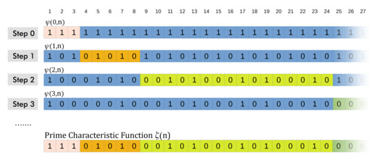
The occurrence of pieces of periodic binary sequences inside the prime characteristic function ${\xi }_p\left(n\right)$ is discussed here. To this end, both the Sieve procedure and a modified version of it are investigated step-by-step, where each step is labelled with the progressive index $k$, with $k=0$ denoting the beginning of the two procedures. The difference between the modified and the true Sieve procedure is simply that in the Sieve procedure, in each step $k\ge 1$, only the multiplies of the prime $p\left(k\right)$ are struck out, but not the prime itself, whereas in the modified Sieve procedure the prime itself is also deleted. As previously stated, the status of each integer (0→deleted, 1→undeleted) is stored in a N-size vector, which is initialized with all $1$ values. The outputs of the Sieve procedure and its modified version are denoted as $\xi (k,n)$ and $\psi (k,n)$, respectively, for each step $k>0$. Consequently, the deletion of an integer from the true or the modified Sieve procedure simply means that a $0$ value replaces a $1$ value in the two previous sequences. In the case of the Sieve procedure, the sequence $\xi (k,n)$ is an approximation at the step $k$ of the prime characteristic function ${\xi }_p\left(n\right)$.

At the beginning of the procedures ($k=0$), we have two equal periodic sequences of all $1$ values, that is, $\xi (0,n)$ and $\psi (0,n)$, whose period is $T\left(0\right)=1$. In the first step of the modified Sieve procedure ($k=1$), the multiples of $p\left(1\right)=2$ are struck out, including $p\left(1\right)$ itself. Consequently, we obtain a sequence $\psi (1,n)$, which is still periodic, with alternating $1$ and $0$ symbols. The period of $\psi (1,n)$ is given by the prime value $p\left(1\right)$ itself, that is, $T\left(1\right)=2$. In the following, $T\left(k\right)$ will denote the period of the sequence $\psi (k,n)$. Conversely, in the Sieve procedure, the prime $p\left(1\right)$ is not deleted. In this case, the output sequence $\xi (1,n)$ is not periodic, but includes a piece of the periodic sequence $\psi (1,n)$, by starting from the square $p{\left(1\right)}^2=4$. Before such a value, the previous sequence $\xi (0,n)$ is preserved, which coincides with $\psi (0,n)$. It follows that $\xi (1,n)$ is a mixed sequence, being composed by pieces of both $\psi (0,n)$ and $\psi (1,n)$, that is,

$$\xi (1,n)=\left\{\begin{array}{cc}\psi (0,n)\hfill & \mathrm{if}p{\left(0\right)}^2\le n<p{\left(1\right)}^2\hfill \\ \psi (1,n)\hfill & \mathrm{if}n\ge p{\left(1\right)}^2.\hfill \end{array}\right.$$

(15)

Similarly, in the second step of the modified Sieve procedure ($k=2$), every multiple of $p\left(2\right)=3$, which is not yet struck out, is deleted, including the prime itself, to give the new sequence $\psi (2,n)$. Therefore, this sequence comes from the deletion of all the multiplies of the primes $p\left(1\right)$ and $p\left(2\right)$, including the primes themselves. It follows that the sequence $\psi (2,n)$ is periodic, with a period equal to the product of $p\left(1\right)$ and $p\left(2\right)$, as it will be demonstrated in Theorem 1. If we consider the second step of the Sieve procedure, where the primes $p\left(1\right)$ and $p\left(2\right)$ have not been deleted, we obtain the sequence $\xi (2,n)$. This is again a mixed sequence, where a piece of the periodic sequence $\psi (2,n)$ is introduced, by starting from the square $p{\left(2\right)}^2=9$, whereas the previous binary values are saved before this square. Consequently, we have

$$\xi (2,n)=\left\{\begin{array}{cc}\psi (0,n)\hfill & \mathrm{if}p{\left(0\right)}^2\le n<p{\left(1\right)}^2\hfill \\ \psi (1,n)\hfill & \mathrm{if}p{\left(1\right)}^2\le n<p{\left(2\right)}^2\hfill \\ \psi (2,n)\hfill & \mathrm{if}n\ge p{\left(2\right)}^2.\hfill \end{array}\right.$$

(16)

In general, the multiples of the prime $p\left(k\right)$, which are not yet struck out in the previous steps, are deleted in the k-th step of the modified Sieve procedure, including the prime $p\left(k\right)$ itself. Consequently, after performing all the first $k$ steps, we obtain the periodic sequence $\psi (k,n)$, as shown in Theorem 1. In the case of the original Sieve procedure, after the k-th step, we obtain the sequence $\xi (k,n)$, which is an approximation of the prime characteristic function until the prime $p\left(k\right)$. Such an approximation differs from the previous one $\xi (k-1,n)$, only by starting from the square $p{\left(k\right)}^2$. In fact, after this point, a piece of the periodic sequence $\psi (k,n)$ is recognizable. It follows that $\xi (k,n)$ can be eventually written as a mixed sequence, which is a generalization of Equations (15) and (16), that is,

$$\xi (k,n)=\left\{\begin{array}{cc}\psi (0,n)\hfill & \mathrm{if}p{\left(0\right)}^2\le n<p{\left(1\right)}^2\hfill \\ \psi (1,n)\hfill & \mathrm{if}p{\left(1\right)}^2\le n<p{\left(2\right)}^2\hfill \\ \dots \hfill \\ \psi (k-1,n)\hfill & \mathrm{if}p{(k-1)}^2\le n<p{\left(k\right)}^2\hfill \\ \psi (k,n)\hfill & \mathrm{if}n\ge p{\left(k\right)}^2.\hfill \end{array}\right.$$

(17)

By evaluating the expression (17), we can recognize that subsets of the periodic binary sequences $\psi (k,n)$ are present, for each $k$, in the related intervals $I\left(k\right)=[p{\left(k\right)}^2,p{(k+1)}^2)$ of the prime characteristic function. This happens until the end of the Sieve procedure, because each $k-th$ interval is not influenced by the deletions done in the following steps. We now show that the sequences $\psi (k,n)$ are periodic and that their periods are given by the product of all the primes up to $p\left(k\right)$.

Theorem 1.

Let be given the binary sequences $\psi (k,n)$, which are generated by the deletion of the multiplies of all the primes up to $p\left(k\right)$, including the primes themselves. Then, the sequences $\psi (k,n)$ are periodic, and their periods $T\left(k\right)$ are given by the product of all the primes up to $p\left(k\right)$, that is,

$$T\left(k\right)=\prod _{i=1}^{k}p\left(i\right)$$

(18)

Proof. 

The deletion of the multiplies of all the primes up to $p\left(k\right)$ gives all the sets, as a function of $k$, of reduced residue systems modulo $T\left(k\right)$, where $T\left(k\right)$ is given by Equation (18). Each set is composed by all the positive integers relatively prime to $T\left(k\right)$, that is, by all the numbers such that $gcd(n,T(k\left)\right)=1$. The quantity of integers in each set is given by the Euler phi function $\varphi \left(T\right(k\left)\right)$, which computes the number of positive integers less than $T\left(k\right)$ and relatively prime to $T\left(k\right)$. However, the sets of reduced residue systems are abelian groups, so that each of them is associated to a principal Dirichlet character function. This is an arithmetical function ${\chi }_1(k,n)$, which is nothing but $\psi (k,n)$, being defined as

$${\chi }_1(k,n)=\left\{\begin{array}{cc}1\hfill & \mathrm{if}gcd(n,T(k\left)\right)=1\hfill \\ 0\hfill & \mathrm{if}gcd(n,T(k\left)\right)>1.\hfill \end{array}\right.$$

(19)

In [8], it is proven that ${\chi }_1(k,n)$ is a periodic sequence, and in particular that

$${\chi }_1(k,n+T\left(k\right))={\chi }_1(k,n)\forall n$$

(20)

This completes the proof. ☐

Table 1. Periods $T\left(k\right)$ of the sequences $\psi (k,n)$, for primes $p\left(k\right)\le p\left(7\right)$, in comparison with the sizes $S\left(k\right)$ of the intervals $I\left(k\right)$. The ratios $S\left(k\right)/T\left(k\right)$ are rapidly decreasing as the prime $p\left(k\right)$ grows.

k	$\mathit{p}\left(\mathit{k}\right)$	$\mathit{p}(\mathit{k}+1)$	$\mathit{I}\left(\mathit{k}\right)$	$\mathit{S}\left(\mathit{k}\right)$	$\mathit{T}\left(\mathit{k}\right)$	$\mathit{S}\left(\mathit{k}\right)/\mathit{T}\left(\mathit{k}\right)$
$\left(0\right)$	$\left(1\right)$	2	$[1,4)$	3	1	$3.000000$
1	2	3	$[4,9)$	5	2	$2.500000$
2	3	5	$[9,25)$	16	6	$2.666667$
3	5	7	$[25,49)$	24	30	$0.800000$
4	7	11	$[49,121)$	72	210	$0.342857$
5	11	13	$[121,169)$	48	$2310$	$0.020779$
6	13	17	$[169,289)$	120	$30030$	$0.003996$
7	17	19	$[289,361)$	72	$510510$	$0.000141$

reports the periods $T\left(k\right)$ of the sequences $\psi (k,n)$, $k=0,\dots ,7$, in comparison with the sizes $S\left(k\right)=p{(k+1)}^2-p{\left(k\right)}^2$ of the intervals $I\left(k\right)$, where subsets of each $\psi (k,n)$ are recognizable. The pseudo-prime $p\left(0\right)=1$ is put in brackets.

By considering the ratios $S\left(k\right)/T\left(k\right)$, it is evident that the periods $T\left(k\right)$ increase much faster than the width of the intervals $S\left(k\right)$. This makes sense because the periodicity of the sequences $\psi (k,n)$ is hardly recognizable by simply investigating the subsets of each $\psi (k,n)$ in the intervals $I\left(k\right)$.

3.2. The Symmetric Sequences of the Runs of Zeroes in the Periods $T\left(k\right)$

In Section 3.1, the prime distribution has been represented as the intersection of an endless number of periodic binary sequences $\psi (k,n)$, whose periods $T\left(k\right)$ rapidly grow, and such that subsets of these sequences can be found in limited intervals $I\left(k\right)$ of the prime characteristic function ${\xi }_p\left(n\right)$. In particular, each of these intervals ranges between the squares of a prime $p\left(k\right)$ and of the successive $p(k+1)$. Consequently, the real primes in each interval $I\left(k\right)$ are given by the $1$ values of the correspondent sequence $\psi (k,n)$. In order to complete this analysis, we now consider the gaps between these primes, by following an established trend in literature. In particular, we are interested to investigate the distributions of the runs of zeros $R\left(k\right)$ in each period $T\left(k\right)$, being the binary sequences $\psi (k,n)$ composed by isolated ones followed by strings, more or less large, of zeroes. It follows that the quantity $R\left(k\right)$ also gives the number of undeleted integers (i.e., isolated ones) in each period $T\left(k\right)$, because the quantity $T\left(k\right)$, for $k\ge 1$, is an even number, so that the last digit of each period is a zero.

Let us consider the Sieve procedure described step-by-step in Section 3.1 and the number of runs of zeroes $R\left(k\right)$ in each period $T\left(k\right)$ of the binary sequences $\psi (k,n)$. For $k=0,1$, we have only one run ($R\left(0\right)=R\left(1\right)=1$), whose sizes are $L(1,0)=1$ and $L(1,1)=2$, respectively. For $k=2$, the deletion of both the multiples of $p\left(1\right)$ and $p\left(2\right)$ give two runs ($R\left(2\right)=2$) in the period $T\left(2\right)=6$, whose sizes are $L(1,2)=4$ and $L(2,2)=2$, respectively, and so on.

Table 2. Runs of zeroes in the periods $T\left(k\right)$ of the sequences $\psi (k,n)$, for primes $p\left(k\right)\le p\left(4\right)$. For each $k$, the number of runs $R\left(k\right)$ and their sizes $L(m,k)$ are reported, with $m=1,\dots ,R\left(k\right)$. Let us notice the symmetry of the runs in each period $T\left(k\right)$. By starting from $k=2$, the symmetry center is given by a run of length $4$, whereas the final run of length $2$ is out of symmetry.

k	$\mathit{p}\left(\mathit{k}\right)$	$\mathit{T}\left(\mathit{k}\right)$	$\mathit{R}\left(\mathit{k}\right)$	$\mathit{L}(\mathit{m},\mathit{k})$
$\left(0\right)$	$\left(1\right)$	1	1	1
1	2	2	1	2
2	3	6	2	4												2
3	5	30	8	6						4						2						4
				2						4						6						2
4	7	210	48	10	2	4	2	4	6	2	6	4	2	4	6	6	2	6	4	2	6	4	6	8	4	2	4
				2	4	8	6	4	6	2	4	6	2	6	6	4	2	4	6	2	6	4	2	4	2	10	2

reports the number of runs $R\left(k\right)$ and their sizes $L(m,k)$, for $k\le 4$, where the index $m$ identifies the specific run and $k$ gives the step of the Sieve procedure. Noticeably, the runs of each period $T\left(k\right)$ are symmetrical around a symmetry center given by a run sized $4$, except for a final run that is sized $2$. Such a trend is expected to be a rule also for the successive steps.

3.3. The Relation Between the Primes in an Interval $I\left(k\right)$ and the Runs in a Period $T\left(k\right)$

For evidencing the relation between each period $T\left(k\right)$ and the correspondent number of runs of zeroes $R\left(k\right)$, we report in

Table 3. Periods $T\left(k\right)$ and related runs of zeroes $R\left(k\right)$ for the primes $p\left(k\right)\le p\left(7\right)$. The special prime $p\left[0\right]=1$ is put in round brackets.

k	$\mathit{p}\left(\mathit{k}\right)$	$\mathit{T}\left(\mathit{k}\right)$	$\mathit{R}\left(\mathit{k}\right)$
$\left(0\right)$	$\left(1\right)$	1	1
1	2	2	1
2	3	6	2
3	5	30	8
4	7	210	48
5	11	2310	480
6	13	30,030	5760
7	17	510,510	92,160

the scores of $R\left(k\right)$ for $k\le 7$.

Such scores also give the number of the integers that have not been struck out by the modified Sieve procedure in the period $T\left(k\right)$, which in turn can be related to the number of undeleted integers (and consequently of the primes) in the correspondent interval $I\left(k\right)$. We will show in Theorem 2 that a correlation exists between $T\left(k\right)$ and $R\left(k\right)$, in such a way the number of primes in each interval $I\left(k\right)$ can be inferred. According on the theory of congruences, Theorem 2 gives the quantity of the integers that have not been struck out (i.e., $R\left(k\right)$) in each period $T\left(k\right)$, that is,

Theorem 2.

Let be given the periodic binary sequences $\psi (k,n)$ defined in Theorem 1, and whose periods are $T\left(k\right)={\prod }_{i=1}^{k}p\left(i\right)$. Then, the number of undeleted integers, that is, the number of runs of zeroes $R\left(k\right)$, in a period $T\left(k\right)$, for $k\ge 1$, is given by

$$R\left(k\right)=\prod _{i=1}^k\left(p\left(i\right)-1\right),k\ge 1$$

(21)

Proof. 

The number of undeleted integers in each period $T\left(k\right)$ is given by the number of integers in the reduced residue systems modulo $T\left(k\right)$, that is, the number of positive integers less than $T\left(k\right)$ and relatively prime to $T\left(k\right)$. Such a value is given by the Euler phi function $\varphi \left(T\right(k\left)\right)$, once computed in $T\left(k\right)$, that is [8]

$$\varphi \left(T\left(k\right)\right)=T\left(k\right)·\prod _{p\left|T\right(k)}\left(1-\frac{1}{p}\right)=T\left(k\right)·\prod _{p\left|T\right(k)}\left(\frac{p-1}{p}\right)=T\left(k\right)·\frac{{\prod }_{i=1}^k\left(p\left(i\right)-1\right)}{{\prod }_{i=1}^{k}p\left(i\right)}=\prod _{i=1}^k\left(p\left(i\right)-1\right)$$

(22)

where $p\left(i\right),i=1,\dots ,k$, are the primes dividing $T\left(k\right)$. ☐

By starting from $p\left(4\right)=7$, Table 1 shows that the interval $I\left(k\right)$ is included in the first period of the sequence $\psi (k,n)$. Consequently, a subset of the undeleted integers $R\left(k\right)$ in each period $T\left(k\right)$ lies in the correspondent interval $I\left(k\right)$, where they are just primes. Therefore, we can infer the quantity of primes $P\left(k\right)$ in each $I\left(k\right)$, by starting from the quantity $R\left(k\right)$ in the correspondent period $T\left(k\right)$. As a first approximation, a simple proportional relationship is investigated. Let us consider the local density $D(k,n)$ of the undeleted integers in the period $T\left(k\right)$, where $D(k,n)$ is computed in sliding intervals $J(k,n)$ whose size is the same of $I\left(k\right)=[p{\left(k\right)}^2,p{(k+1)}^2)$, that is, $p{(k+1)}^2-p{\left(k\right)}^2$. In this context, the index $n$ represents the starting point of each $J(k,n)$. If such intervals span the whole period $T\left(k\right)$, we assume that the density $D(k,n)$ is not a function of $n$. In this case, it is equal to the average density $\overline{D}\left(k\right)$ over $T\left(k\right)$, and we have

$$D(k,n)=\overline{D}\left(k\right)=\frac{R\left(k\right)}{T\left(k\right)}=\frac{{\prod }_{i=1}^k\left(p\left(i\right)-1\right)}{{\prod }_{i=1}^{k}p\left(i\right)}=\prod _{i=1}^k\frac{p\left(i\right)-1}{p\left(i\right)},k\ge 1$$

(23)

It is noteworthy that the product structure in Equation (23) is the same as in Equation (12). Let us suppose that the previous assumption holds. Then, an estimation of the local density $D(k,n)$ in each interval $I\left(k\right)$ (that is, for $n=p{\left(k\right)}^2$), will be just the average density $\overline{D}\left(k\right)$ over the period $T\left(k\right)$. Consequently, we can write

$$D\left(k,p{\left(k\right)}^2\right)\simeq \overline{D}\left(k\right),k\ge 1.$$

(24)

Therefore, by starting from Equation (23), we can estimate the quantity of primes $P\left(k\right)$ in each interval $I\left(k\right)$, for $k\ge 1$. To this end, the average density $\overline{D}\left(k\right)$ is multiplied by the size $S\left(k\right)=p{(k+1)}^2-p{\left(k\right)}^2$, that is,

$$P\left(k\right)=\overline{D}\left(k\right)·S\left(k\right)=(p{(k+1)}^2-p{\left(k\right)}^2)·\prod _{i=1}^k\frac{p\left(i\right)-1}{p\left(i\right)},k\ge 1.$$

(25)

Evidently, Equation (25) is analogous to Equation (12), apart from the size $N$ of the global interval $I_N$, where $N\in I_K=[p{\left(K\right)}^2,p{(K+1)}^2)$, that is changed into the size $p{(k+1)}^2-p{\left(k\right)}^2$ of the local interval $I\left(k\right)$.

3.4. The Novel LINPES Estimation of the Prime Number Function $\pi \left(x\right)$

Equation (25) gives a succession of estimations $P\left(k\right)$ of the real number of primes $\pi \left(k\right)$ in each interval $I\left(k\right)=[p{\left(k\right)}^2,p{(k+1)}^2)$. Therefore, the next step will be to blend all these scores to compute a global estimation ${\pi }_P\left(N\right)$ of the quantity of the primes up to $N$, where $N\in I\left(K\right)$, analogously to Equation (12). In theory, ${\pi }_P\left(N\right)$ is simply computable by adding all the contributions $P\left(k\right)$ of Equation (25), for $k=1,\dots ,K$, where $p\left(K\right)$ is the greatest prime number not exceeding $N^{1/2}$. However, such a procedure includes the term $p(K+1)$, which is unknown. In order to overcome this issue, the computation of ${\pi }_P\left(N\right)$ has to involve only the terms up to $P(K-1)$, plus a final term $P(K,N)$, where the interval $I_K$ is only partially considered. Consequently, we obtain

$${\pi }_P\left(N\right)=\sum _{k=0}^{K-1}P\left(k\right)+P(K,N)=P\left(0\right)+\sum _{k=1}^{K-1}\left[\left(p{(k+1)}^2-p{\left(k\right)}^2\right)·\prod _{i=1}^k\frac{p\left(i\right)-1}{p\left(i\right)}\right]+P(K,N)$$

(26)

where $P\left(0\right)=p{\left(1\right)}^2-p{\left(0\right)}^2$, and $P(K,N)=\left(N-p{\left(K\right)}^2\right)·{\prod }_{i=1}^K\frac{p\left(i\right)-1}{p\left(i\right)}$. Let us notice that Equation (26) includes as many contributions as the primes are, where each term is given by a relation similar to Equation (12), with the global size $N$ that is replaced by the size of the interval $I\left(k\right)$. Each contribution includes an average number of primes that is given by ${\prod }_{i=1}^k\frac{p\left(i\right)-1}{p\left(i\right)}$, so that the average distance $p(k+1)-p\left(k\right)$ between two consecutive primes is ${\prod }_{i=1}^k\frac{p\left(i\right)}{p\left(i\right)-1}$, which is of the order of magnitude of $\log \left(p\right(k\left)\right)$. For the Cramér conjecture [15], this average distance is $p(k+1)-p\left(k\right)=\mathcal{O}({\log }^2\left(p\left(k\right)\right)$. Another conjecture by Cramér, by starting from the Riemann’s hypothesis, was $p(k+1)-p\left(k\right)=\mathcal{O}(\sqrt{p\left(k\right)}\log \left(p\left(k\right)\right)$ [12,16]. Consequently, the error given by neglecting the partial term $P(K,N)$ is smaller than the loading term of the Cramér conjectures, so that the partial term $P(K,N)$ could be omitted.

3.5. The Corrected LINPES Estimation by Using the Equivalence with the $Li\left(x\right)$ Function

We want now to show that Equations (3) and (26) are related. To this end, we write the logarithmic integral function $\mathrm{Li}\left(N\right)$ as a summation of integrals, each of them is computed in the interval $I\left(k\right)=[p{\left(k\right)}^2,p{(k+1)}^2)$, that is,

$$\mathrm{Li}\left(N\right)={\int }_2^{p{\left(1\right)}^2}\frac{dt}{\log t}+\sum _{k=1}^{K-1}{\int }_{p{\left(k\right)}^2}^{p{(k+1)}^2}\frac{dt}{\log t}+{\int }_{p{\left(K\right)}^2}^N\frac{dt}{\log t},$$

(27)

where the first term starts from $2$ to cope with a possible improper integral, and $p{\left(K\right)}^2$ is the greatest square of a prime less than $N$. Consequently, the $\mathrm{Li}\left(N\right)$ function is expressed by Equation (27) as a succession of estimations $L\left(k\right)$, in a similar way to Equation (26), that is,

$$\mathrm{Li}\left(N\right)=L\left(0\right)+\sum _{k=1}^{K-1}L\left(k\right)+L(K,N),$$

(28)

where $L\left(0\right)={\int }_2^{p{\left(1\right)}^2}\frac{dt}{\log t}$, $L(K,N)={\int }_{p{\left(K\right)}^2}^N\frac{dt}{\log t}$, and

$$L\left(k\right)={\int }_{p{\left(k\right)}^2}^{p{(k+1)}^2}\frac{dt}{\log t}.$$

(29)

We now apply the Mean Value Theorem to each interval $I\left(k\right)$ in Equation (27), that is,

$$\mathrm{Li}\left(N\right)=\frac{p{\left(1\right)}^2-2}{\log \left({\varsigma }_0\right)}+\sum _{k=1}^{K-1}\frac{p{(k+1)}^2-p{\left(k\right)}^2}{\log \left(\varsigma \left(k\right)\right)}+\frac{N-p{\left(K\right)}^2}{\log \left({\varsigma }_K\right)},$$

(30)

where ${\varsigma }_0\in I\left(0\right)$, $I\left(0\right)=[p{\left(0\right)}^2,p{\left(1\right)}^2)$, $\varsigma \left(k\right)\in I\left(k\right),k=1,\dots ,K-1$, and ${\varsigma }_K\in I(K,N)$, $I(K,N)=[p{\left(K\right)}^2,N)$. In order to show the equivalence between the Equations (26) and (30), we also consider the lower bound $p{\left(k\right)}^2$ of the interval $I\left(k\right)$. By taking, in the two summations, the ratio between the two terms multiplying the interval size $S\left(k\right)=p{(k+1)}^2-p{\left(k\right)}^2$, we can write

$$\frac{{\prod }_{i=1}^k\frac{p\left(i\right)-1}{p\left(i\right)}}{\frac{1}{\log \left(\varsigma \left(k\right)\right)}}={\left(\frac{{\prod }_{i=1}^k\frac{p\left(i\right)}{p\left(i\right)-1}}{\log \left(\varsigma \left(k\right)\right)}\right)}^{-1}$$

(31)

From Equation (13), we have

$$\underset{k\to \infty }{\lim }\frac{{\prod }_{i=1}^k\frac{p\left(i\right)}{p\left(i\right)-1}}{\log \left(\varsigma \left(k\right)\right)}=\underset{k\to \infty }{\lim }\left[\frac{{\prod }_{i=1}^k\frac{p\left(i\right)}{p\left(i\right)-1}}{\log \left(p{\left(k\right)}^2\right)}\times \frac{\log \left(p{\left(k\right)}^2\right)}{\log \left(\varsigma \left(k\right)\right)}\right]=\frac{1}{2}\times e^{\gamma }\times \underset{k\to \infty }{\lim }\frac{\log \left(p{\left(k\right)}^2\right)}{\log \left(\varsigma \left(k\right)\right)}$$

(32)

where $\varsigma \left(k\right)\in I\left(k\right)=[p{\left(k\right)}^2,p{(k+1)}^2)$, so that its maximum distance from $p{\left(k\right)}^2$ is $p{(k+1)}^2-p{\left(k\right)}^2$. However, we know that the $k-th$ prime $p\left(k\right)$ is given asymptotically by $p\left(k\right)\sim klog\left(k\right)$ [9]. Therefore, $p{\left(k\right)}^2\sim k^2·log{\left(k\right)}^2$ and $p{(k+1)}^2\sim {(k+1)}^2·log{(k+1)}^2\sim k^{2}log{\left(k\right)}^2$, so that for each point $\varsigma \left(k\right)\in [p{\left(k\right)}^2,p{(k+1)}^2)$ we have $\varsigma \left(k\right)\sim k^{2}log{\left(k\right)}^2$. It follows that

$$\underset{k\to \infty }{\lim }\frac{{\prod }_{i=1}^k\frac{p\left(i\right)}{p\left(i\right)-1}}{\log \left(\varsigma \left(k\right)\right)}=\frac{1}{2}\times e^{\gamma }\times \underset{k\to \infty }{\lim }\frac{\log \left(p{\left(k\right)}^2\right)}{\log \left(\varsigma \left(k\right)\right)}=\frac{1}{2}\times e^{\gamma }=\frac{1}{c}\simeq 0.8905$$

(33)

and consequently Equation (31) gives, for each fixed $k$,

$$\frac{{\prod }_{i=1}^k\frac{p\left(i\right)-1}{p\left(i\right)}}{\frac{1}{\log \left(\varsigma \left(k\right)\right)}}=c_I\left(k\right)\mathrm{where}\underset{k\to \infty }{\lim }{c}_I\left(k\right)=c=2\times e^{-\gamma }\simeq 1.1229.$$

(34)

It follows that the trends of the two estimations (26) and (30) are the same as $k\to \infty$, apart from the constant coefficient $c$. Due to this multiplicative factor, the proposed estimation (26) overestimates the prime number function $\pi \left(N\right)$ with respect to Equation (30), and in this sense it is similar to the heuristic procedure described in Section 2. However, it has to be noticed that this last one is completely probabilistic, whereas the proposed method is also based on an analytical procedure, that is, the recognition of an infinite number of binary periodical sequences and related intervals of the prime characteristic function. In order to correct this discrepancy, we relax the conjecture of Section 3.3, in such a way the trend of the local density $D(k,n)$ becomes a function of $n$. Experimentally, the values of the local density $D(k,p_k^2)$ in the interval $I\left(k\right)$ are lower than those of the average density $\overline{D}\left(k\right)$. The following conjecture is then proposed, which links $D(k,p_k^2)$ and $\overline{D}\left(k\right)$ by means of the constant $c$ of the Third Mertens’ Theorem [11].

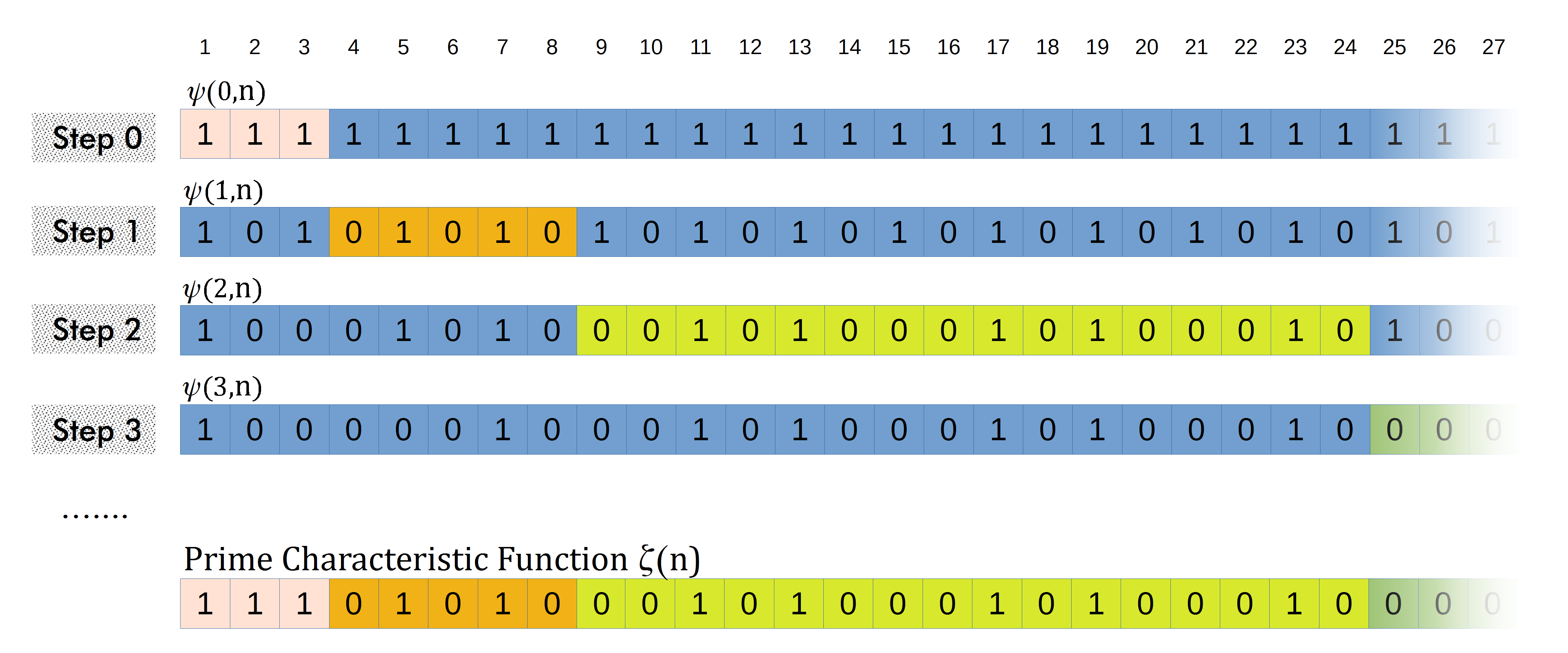
Conjecture 1.

The local density $D(k,n)$ of the undeleted integers in the period $T\left(k\right)$, if computed in sliding intervals whose size is the same of $I\left(k\right)=[p{\left(k\right)}^2,p{(k+1)}^2)$, is a function of the starting point $n$ of the sliding interval. In particular, the average density $\overline{D}\left(k\right)$ is greater than the local density $D\left(k,p{\left(k\right)}^2\right)$ in the interval $I\left(k\right)$, in such a way the succession $c_I\left(k\right)$ of their ratios exceeds the unity. Moreover, the limit value as $k\to \infty$ of $c_I\left(k\right)$ is equal to the constant $c=2·e^{-\gamma }\simeq 1.1229$ of the Third Mertens’ Theorem, that is,

$$\underset{k\to \infty }{\lim }\frac{\overline{D\left(k\right)}}{D\left(k,p_k^2\right)}=c.$$

(35)

The typical trend of $D(k,n)=D(16,n)=D\left(n\right)$, for $k=16$ and varying $n$, is plotted in Figure 1, together with the average density $\overline{D}\left(k\right)=\overline{D}\left(16\right)=\overline{D}$ in the period $T\left(k\right)=T\left(16\right)$. Let us notice that, as it will be discussed in the following, such a trend is less appreciable for small values of the primes.

Figure 1 can be explained as follows. Let us consider the sequences $\psi (k,n)$ defined in Section 3.1, where the multiples of the primes up to $p\left(k\right)$ have been struck out, included the primes themselves. In each of these sequences, all the undeleted integers are just primes in the range $[p(k+1),p{(k+1)}^2]$, whereas the undeleted integers greater than $p{(k+1)}^2$ can be indifferently primes or composites, because the multiples of the primes greater than $p\left(k\right)$ have not yet been struck out.

At the beginning of the modified Sieve procedure ($k=0$), the local density $D(k,n)$ of the undeleted integers is not a function of $n$, because no integer has been still struck out. In the first step ($k=1$), only the even integers (i.e., the multiplies of $p\left(1\right)=2$) have been struck out, so that $D(k,n)$ is still a constant value up to infinity. Noticeably, the multipliers (i.e. the integers multiplying $p\left(1\right)$ to give the deleted multiplies) are equal to the undeleted integers when the procedure starts (i.e., all the integers). This rule also holds for the following steps, that is, the multipliers of the prime $p\left(k\right)$ in the $k-th$ step of the modified Sieve procedure are equal to the undeleted integers in the previous $(k-1)-th$ step. It follows that the multipliers of $p\left(2\right)=3$ are all the odd integers, whose distribution is again uniform. Some of these multipliers (that is, $3,5,7$) are just primes in the interval $\left[p\left(2\right),p{\left(2\right)}^2\right)$, but they can also be composites beyond $p{\left(2\right)}^2$. In this case, the distribution of the composite multipliers exactly compensate the decreasing trend of the distribution of the multipliers that are also prime numbers. If the primes $p\left(k\right)$ are sufficiently small, such a compensation happens quickly, because it starts from $p{\left(k\right)}^2$. In these cases, the distribution of the local density $D(k,n)$ is still approximately uniform. However, as $p\left(k\right)$ grows, a transient state is noticeable, because, for such values of $k$ and small values of $n$, the local density $D(k,n)$ is greater than the average density $\overline{D}\left(k\right)$. In fact, for such $n$ values, only a portion of the multiplies of the primes $p\left(i\right),i=1,\dots ,k$, have been struck out, because the deletion of the multiplies of the prime $p\left(i\right),i<k$, starts only from $p{\left(i\right)}^2$, apart from the prime $p\left(i\right)$ itself. This means that the deletion of the multiplies of $p\left(i\right),i=1,\dots ,k$, is completed only at the lower bound of the interval $I\left(k\right)$, that is, $p{\left(k\right)}^2$. Consequently, after this point, the transient state ends and the stationary state begins, where the local density $D(k,n)$ fluctuates around the average density $\overline{D}\left(k\right)$.

Figure 1 shows the trend of the local density $D(k,n)$ in the case of $p\left(k\right)=16$. Starting approximately from this value of $k$, we can notice a minimum value $D(k,p{\left(k\right)}^2)$ for the distribution of $D(k,n)$, which is located immediately after the transient state, that is, at the lower bound of the interval $I\left(k\right)$. Such a minimum value is about a 10 percent lower than the average density $\overline{D}\left(k\right)$. In fact, as previously explained, the multipliers of the prime $p\left(k\right)$ are just primes up to $p{\left(k\right)}^2$, whereupon they can be even composites. It follows that the distribution of the composite multipliers compensate the decreasing distribution of the multipliers that are prime numbers only starting from the multiple $p{\left(k\right)}^3=p{\left(k\right)}^2·p\left(k\right)$. Therefore, as $k\to \infty$, such a compensation is delaying, in such a way the ratio between $\overline{D}\left(k\right)$ and $D(k,n)$ more and more grows up to the $c$ value of Equation (35). As a matter of fact, if all the multipliers were primes, their distribution would decrease by following a logarithmic trend, so that $D(k,n)$ would augment with the same trend, by starting from the minimum value in the interval $I\left(k\right)$. In the real case, however, the compensation given by the composite multipliers has the effect that the local density does not grow indefinitely, but tends to the limit value $c·D(k,p{\left(k\right)}^2)$. Let us notice that, if we stop the procedure to a finite value of $k$, the ratio between $\overline{D}\left(k\right)$ and $D(k,n)$ is $c_I\left(k\right)·D(k,p{\left(k\right)}^2)$, where the succession $c_I\left(k\right)$ is increasing and tends to the limit value $c$ as $k\to \infty$.

In order to evaluate the effect of the compensation delay for the small primes $p\left(k\right)$, $k=1,\dots ,7$, in comparison with the case of $p\left(16\right)=53$,

Table 4. Prime numbers $p\left(k\right),k=1,\dots ,7$, and $k=16$, and the related intervals $I\left(k\right)$, together with: a) the multipliers $f_I$ such that the multiples $f_I·p\left(k\right)$ lie inside the intervals $I\left(k\right)$; b) the first multiplier $f_c$ that is a composite number. Let us notice that the difference between $f_c$ and the multipliers $f_I$ rapidly grows, so that the distance between the multiple $f_c·p\left(k\right)$ and the upper bound of the interval $I\left(k\right)$ becomes larger and larger.

k	$\mathit{p}\left(\mathit{k}\right)$	$\mathit{I}\left(\mathit{k}\right)$	${\mathit{f}}_{\mathit{I}}|({\mathit{f}}_{\mathit{I}}·\mathit{p}\left(\mathit{k}\right))\in \mathit{I}\left(\mathit{k}\right)$	${\mathit{f}}_{\mathit{c}}$	${\mathit{f}}_{\mathit{c}}·\mathit{p}\left(\mathit{k}\right)$
1	2	$[4,9)$	$2;3$	4	8
2	3	$[9,25)$	$3;5;7$	9	27
3	5	$[25,49)$	$5;7$	25	125
4	7	$[49,121)$	$7;11;13;17$	49	343
5	11	$[121,169)$	$11;13$	121	1331
6	13	$[169,289)$	$13;17;19$	169	2197
7	17	$[289,361)$	$17;19$	289	4913
16	53	$[2809,3481)$	$53;59;61$	2809	148,877

reports: a) the multipliers $f_I$ such that the multiples $f_I·p\left(k\right)$ lie in the interval $I\left(k\right)=[p{\left(k\right)}^2,p{(k+1)}^2)$, and b) the first multiplier that is a composite number, that is, $f_c=p{\left(k\right)}^2$, whose correspondent multiple is $p{\left(k\right)}^2·p\left(k\right)=p{\left(k\right)}^3$. Evidently, as $k$ grows, the difference between the upper bound $p{(k+1)}^2$ of $I\left(k\right)$ and $p{\left(k\right)}^3$ becomes so large that the compensation effect of the composite multipliers is no longer noticeable in the interval itself.

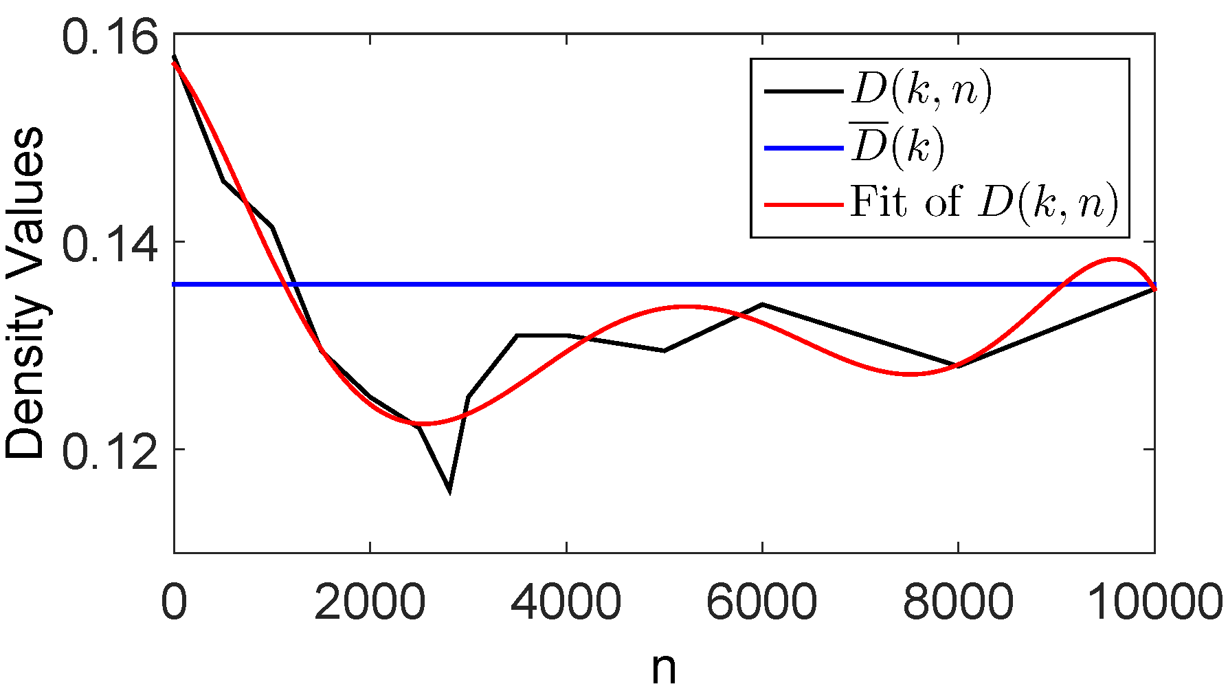
Figure 2 shows the trend of the succession $c_I\left(k\right)$, as $k$ approaches infinity. Evidently, such a succession tends to the constant value $c$. The x-axis is in a logarithmic scale, in such a way the values of $p{\left(k\right)}^2$ can be visualized up to ${10}^{15}$.

Finally,

Table 5. Parameters and coefficients of determination of the linear regressions $y_i=m_1{x}_i+q_1$ of the proposed estimations $P\left(k\right)$ versus the logarithmic-integral ones $L\left(k\right)$, together with the parameters and coefficients of determination of the linear regressions $y_i=m_2{x}_i+q_2$ of $P\left(k\right)$ versus the true number of primes $\pi \left(k\right)$. Each point is computed in an interval $I\left(k\right)$.

k	$\mathit{p}{\left(\mathit{k}\right)}^2$	${\mathit{m}}_1$	${\mathit{q}}_1$	${\mathit{R}}_1^2$	${\mathit{m}}_2$	${\mathit{q}}_2$	${\mathit{R}}_2^2$
$[1,168]$	$(1,{10}^6)$	$0.894209$	$1.2846$	$0.9999932989$	$0.894649$	$0.2597$	$0.9996747582$
$[169,446]$	$({10}^6,{10}^7)$	$0.892762$	$0.7754$	$0.9999985384$	$0.894052$	$-2.5697$	$0.9998452835$
$[447,1229]$	$({10}^7,{10}^8)$	$0.891565$	$1.0381$	$0.9999997462$	$0.891906$	$-2.2200$	$0.9999418064$
$[1230,3401]$	$({10}^8,{10}^9)$	$0.891025$	$2.1044$	$0.9999999196$	$0.891016$	$2.0534$	$0.9999821107$
$[3402,9592]$	$({10}^9,{10}^{10})$	$0.890801$	$2.2963$	$0.9999999842$	$0.890751$	$5.6943$	$0.9999941659$
[9593, 27,293]	$({10}^{10},{10}^{11})$	$0.890657$	$4.9719$	$0.9999999945$	$0.890664$	$2.8478$	$0.9999981622$
[27,294, 78,498]	$({10}^{11},{10}^{12})$	$0.890606$	$5.7853$	$0.9999999989$	$0.890606$	$5.6440$	$0.9999993974$
[78,499, 227,647]	$({10}^{12},{10}^{13})$	$0.890570$	$10.3672$	$0.9999999997$	$0.890569$	$13.0142$	$0.9999998112$
[227,648, 664,579]	$({10}^{13},{10}^{14})$	$0.890555$	$14.8795$	$0.9999999999$	$0.890555$	$13.7581$	$0.9999999398$
[664,580, 1,951,957]	$({10}^{14},{10}^{15})$	$0.890546$	$20.1618$	$1.0000000000$	$0.890546$	$27.3660$	$0.9999999808$

highlights the equivalence between the proposed estimation (26) and the logarithmic-integral one (3). To this end, a number of linear regressions have been computed between the occurrences $P\left(k\right)$ (25) in each interval $I\left(k\right)$ of the proposed estimation versus the correspondent ones $L\left(k\right)$ (29) of the integral-logarithmic function. Each row of Table 5 is referred to the prime squares $p{\left(k\right)}^2$ ranging from a power-of-ten to the following one, except the first raw, which includes all the squares lower than ${10}^6$, in order to elaborate a sufficient number of points. For each of these ranges, we report the coefficients $m_1$ and $q_1$ of the linear regressions $y_i=m_1{x}_i+q_1$, together with the coefficient of determination $R_1^2$, which is a measure of the fitting between the two estimations. Evidently, the coefficient of determination tends very fast to its optimal value, that is $1$, despite that the number of observations has increased. Let us notice that the intercept $q_1$ is practically negligible with respect to the full-scale level, whereas the slope $m_1$ is approaching the constant value $1/c$.

For comparison, Table 5 also reports the parameters and the coefficient of determination in the case of the linear regressions $y_i=m_2{x}_i+q_2$ concerning the occurrences $P\left(k\right)$ versus the targets $\pi \left(k\right)$. These scores are defined as the number of primes in each interval $I\left(k\right)$. Even in this case, the fitting between $P\left(k\right)$ and $\pi \left(k\right)$ is impressive, as shown by the coefficient of determination $R_2^2$. Noticeably, the slope $m_2$ still approaches the value $1/c$, because the P.N.T. guarantees that the logarithmic-integral function and the prime number function goes to infinity in the same way.

From the previous analysis, it follows that, for a given $N$, the proposed approximation ${\pi }_P\left(N\right)$ overestimates the prime number function $\pi \left(N\right)$ by a factor $c_N$, which can be computed by considering that we have an overestimation for each interval $I\left(k\right)$ that can be computed by considering a factor in the finite set $c_I\left(k\right),k=1,\dots ,K$, where $K$ is such that $N\simeq p{\left(K\right)}^2$ (see Equation (34)). If $N\to \infty$, the overestimation factor $c_N$ tends to the constant $c$. Being $c_N$ unknown, an adjusted version (36) of (26) can be defined by means of the correction factor $1/c$, that is,

$$\begin{array}{c}{\tilde{\pi }}_P\left(N\right)=\frac{1}{c}·\left(P_0+\sum _{k=1}^{K-1}P\left(k\right)+P_{K,N}\right)=\hfill \\ =\frac{1}{c}·\left(p{\left(1\right)}^2-p{\left(0\right)}^2\right)+\frac{1}{c}·\sum _{k=1}^{K-1}\left[\left(p{(k+1)}^2-p{\left(k\right)}^2\right)·\prod _{i=1}^k\frac{p\left(i\right)-1}{p\left(i\right)}\right]+\frac{1}{c}·\left(N-p{\left(K\right)}^2\right)·\prod _{i=1}^K\frac{p\left(i\right)-1}{p\left(i\right)}.\hfill \end{array}$$

(36)

Clearly, the corrected version ${\tilde{\pi }}_P\left(N\right)=\frac{1}{c}·{\pi }_P\left(N\right)$ is able to give better estimations than ${\pi }_P\left(N\right)$ as $N$ approaches infinity. In order to give a quantitative assessment,

Table 6. The proposed estimation ${\pi }_P\left(N\right)$ and its adjusted version ${\tilde{\pi }}_P\left(N\right)$ in comparison with the logarithmic integral estimation $\mathrm{Li}\left(N\right)$, and the prime number function $\pi \left(N\right)$. The scores of $\mathrm{Li}\left(N\right)$ have been computed by using the MATLAB^® toolbox. The scores of ${\pi }_P\left(N\right)$ and ${\tilde{\pi }}_P\left(N\right)$ have been rounded to the nearest integer.

$\mathit{N}={10}^{\mathit{i}}$	$\mathit{\pi }\left(\mathit{N}\right)$	$\mathbf{Li}\left(\mathit{N}\right)$	${\mathit{\pi }}_{\mathit{P}}\left(\mathit{N}\right)$	${\tilde{\mathit{\pi }}}_{\mathit{P}}\left(\mathit{N}\right)$
${10}^1$	4	6	4	4
${10}^2$	25	30	27	24
${10}^3$	168	178	181	161
${10}^4$	1229	1246	1348	$1200$
${10}^5$	9592	9630	10,639	$9474$
${10}^6$	78,498	78,628	87,688	$78090$
${10}^7$	664,579	664,918	744,175	662,715
${10}^8$	5,761,455	5,762,209	6,460,497	5,753,306
${10}^9$	50,847,534	50,849,235	57,056,721	50,811,064
${10}^{10}$	455,052,511	455,055,615	510,796,987	454,883,106
${10}^{11}$	4,118,054,813	4,118,066,401	4,623,402,885	4,117,306,712
${10}^{12}$	37,607,912,018	37,607,950,281	42,226,535,908	37,604,250,381
${10}^{13}$	346,065,536,839	346,065,645,810	388,584,655,120	346,048,624,432
${10}^{14}$	3,204,941,750,802	3,204,942,065,692	3,598,796,310,868	3,204,857,671,495
${10}^{15}$	29,844,570,422,669	29,844,571,475,288	33,512,578,849,645	29,844,157,918,447

reports the scores of ${\pi }_P\left(N\right)$ (26) and of its adjusted version ${\tilde{\pi }}_P\left(N\right)$ (36), in comparison with the logarithmic integral estimation $\mathrm{Li}\left(N\right)$ (27), and with the prime number function $\pi \left(N\right)$. The range of each row of Table 6 starts from a power-of-ten and ends to the following one up to ${10}^{15}$.

It can be noticed that the scores of ${\tilde{\pi }}_P\left(N\right)$ slightly underestimate both the true number of primes $\pi \left(N\right)$ and the logarithmic integral function $\mathrm{Li}\left(N\right)$, which, in turn, is such that the sign of its difference with ${\tilde{\pi }}_P\left(N\right)$ changes infinitely many times [17,18], by showing some irregularities in the distribution of the primes [19], which have been investigated by considering differences in some subsets of the primes themselves [20]. Concerning the previous underestimation, this is due to the fact that the limit value $c$ is an upper bound for the succession $c_I\left(k\right)$. Evidently, ${\tilde{\pi }}_P\left(N\right)$ would be perfectly accurate if the terms $c_I\left(k\right)$ were available for the computation of (36), by considering the real number of primes in each interval $I\left(k\right)$.

4. An Extension of the Procedure to the Twin Prime Numbers

4.1. Preliminary Concepts

Two prime numbers $p$ and $q$ are twin primes if $|p-q|=2$, which is the lowest possible distance between primes, apart from $p=2$ and $q=3$, where $|p-q|=1$. Let us note that two consecutive pairs of twin primes do not ever occur, apart from the case $\{3,5\}$ and $\{5,7\}$. In fact, one number in the sequence $\{n,n+2,n+4\}$ is certainly a multiple of 3. The gaps between consecutive primes have been extensively investigated in literature [13,15,21]. However, differently from the primes, it is presently unknown whether there are infinitely many pairs of twin primes. In any case, a preliminary counting shows that the twin primes are relatively abundant into the sequence of primes, and, consequently, it is reasonable to infer the so-called twin prime conjecture, which states that there are infinitely many pairs of twin primes. This conjecture is strengthened by the fact that the distribution of the primes does not change abruptly. Recently, significant progress has been made by showing that $\underset{k\to \infty }{\lim \inf }\left[p(k+1)-p\left(k\right)\right]=\ell <\infty$, that is, a finite upper bound exists for the limit inferior of the difference between consecutive primes. In particular, Zhang found that $\ell \le 7·{10}^7$ [22], and this bound has been successively improved by Maynard to $\ell \le 600$ [23]. Finally, the Polymath’s project, whose aim is to collect all the various efforts that try to put the bound lower as much as possible, has reached the value of $\ell \le 246$ [24]. Evidently, in order to demonstrate the twin prime conjecture, a bound of $\ell =2$ should be obtained. In this work, we try to give a contribution to the discussion of this conjecture, by following a different strategy, that is, by exploiting the concepts previously introduced for the primes. Consequently, as for the primes, the approach is not merely probabilistic, but also analytic, so constituting a possible significant step for further advancements, as in the case of approaches based on periodic functions [25]. The distribution of the twin primes is commonly characterized by using the twin prime function ${\pi }_2\left(x\right)$ (6). Such a distribution decays more rapidly than the distribution of the primes. In fact, Brun demonstrated in 1919 [26] that, if $S_T$ is the set of twin primes given by $S_T=\{p:p\mathrm{prime}\mathrm{and}p+2\mathrm{prime}\}$, the related series of the reciprocals converges to the finite limit $B\simeq 1.9022$ [1], that is,

$$\sum _{p\in S_T}\left(\frac{1}{p}+\frac{1}{p+2}\right)=B$$

(37)

regardless of the fact of whether the number of summation terms is infinite or not, whereas the same summation instead diverges for the primes.

Analogously to the P.N.T., a possible function for approximating the twin prime function ${\pi }_2\left(x\right)$ has been proposed [5] as the logarithmic integral function ${\mathrm{Li}}_2\left(x\right)$ (8). As for the primes, we want to obtain an equivalent procedure and investigate possible consequences.

4.2. A Possible Relation Between the Twin Primes in the Intervals and the Undeleted Integers in the Periods

In Section 3.2, the distribution of the runs into each period $T\left(k\right)$ has been investigated. In the present analysis, the same investigation can be made for the particular case in which the size of the runs is $2$. Evidently, such an investigation can potentially give an estimation of the quantity of twin primes, similarly to the one given by the Equation (26) for the primes. In fact, we will suggest that the number of the runs sized $2$ in the interval $I\left(k\right)$ is equal to the quantity of twin primes in the same interval. Such a number is equal to the number of $\left\{101\right\}$ sequences, if the sequence $\left\{10\right\}$ is completely included in the interval. However, such a sequence cannot occur across two intervals, because each interval, apart from the first one, ends with an even number (that is, a $0$), because it is followed by a square of an odd prime (that is, another $0$), which is an odd number. For the sake of clarity, in the following we denote the runs sized $2$ as runs $2$. Let us notice that this procedure can be extended to run-lengths of whatever size, by following the Hardy-Littlewood conjecture B [6]. Such a topic will be the object of future explorations.

Table 7. Number of runs $2$, denoted as $R_2\left(k\right)$, that are included in the periods $T\left(k\right)$, for $p\left(k\right),k=0,\dots ,7$. These scores are compared with the total number of runs $R\left(k\right)$. The special prime $p\left(0\right)=1$ is put in round brackets.

k	$\mathit{p}\left(\mathit{k}\right)$	$\mathit{T}\left(\mathit{k}\right)$	$\mathit{R}\left(\mathit{k}\right)$	${\mathit{R}}_2\left(\mathit{k}\right)$
$\left(0\right)$	$\left(1\right)$	1	1	0
1	2	2	1	1
2	3	6	2	1
3	5	30	8	3
4	7	210	48	15
5	11	2310	480	135
6	13	30,030	5760	1485
7	17	510,510	92,160	22,275

reports the number $R_2\left(k\right)$ of the runs $2$ in each period $T\left(k\right)$ for $p\left(k\right),k=0,\dots ,7$. As for the total number of runs $R\left(k\right)$ (21) in the same period, a correlation can be found between $R_2\left(k\right)$ and the prime number $p\left(k\right)$. In particular, the scores of Table 7 suggest the following conjecture for $R_2\left(k\right)$

$$R_2\left(k\right)=\prod _{i=2}^k(p\left(i\right)-2),k\ge 2.$$

(38)

Equation (38) can be investigated by taking the modified Sieve procedure. At the start of the procedure ($k=0$), we have no run $2$. In the first step ($k=1$), the multiples of $p\left(1\right)=2$ are struck out, in such a way the sequence $\psi (1,n)$ is made by runs $2$ only. In particular, a single run $2$ is included in the period $T\left(1\right)=2$, so that $R_2\left(1\right)=1$. For $k=2$, we delete the multiples of $p\left(2\right)=3$, so that the period $T\left(2\right)=6$ becomes three times greater. This implies that the number of runs $2$ could increase from $1$ to $3$, but the deletion in the point $n=3$ vanishes two of these runs. Let us notice that the cancellation of one multiple vanishes two runs $2$ only in this step, being all the runs $2$ consecutive, but this does not happen in the following steps, where only one run $2$, or even none, is deleted at the time. It follows that $R_2\left(2\right)=1$, as in the previous step. On the whole, we obtain that the deleted runs $2$ in the period $T\left(2\right)$ are a fraction $2/3=2/p\left(2\right)$ of the total number of runs $2$ in the same period if no cancellations were made.

Similarly, for $k=3$, the multiples of $p\left(3\right)=5$ are struck out, so that the period $T\left(3\right)$ becomes five times greater. It follows that the number of runs $2$ would grow from $1$ to $5$, but two cancellations (for $n=5,25$) vanish two of the five runs $2$. Consequently, we obtain $R_2\left(3\right)=3$ and the fraction of the deleted runs $2$ is $2/5=2/p\left(3\right)$ of the total runs in this period if no cancellation were made. In this step, all the cancellations imply the deletion of one run $2$, but this will not also be a rule for the following steps. In fact, for $k=4$, we have eight cancellations in the period $T\left(4\right)$, but only six of them stroke out a run $2$. However, the fraction of the deleted runs $2$ in the period is still given by $6/21=2/7=2/p\left(4\right)$ of the pre-existing ones before the cancellations, being $R_2\left(4\right)=3·7-6=15$.

In the case of primes, it follows from the relation (21) that we struck out, in each step, a fraction $1/p\left(k\right)$ of the total number of runs in the period $T\left(k\right)$ if no cancellations were made, which is given by the product of the prime $p\left(k\right)$ by the actual number of runs in the previous period $T(k-1)$. By considering the scores of Table 7, a similar relation can be conjectured for the runs $2$ in the case of twin primes, in order to link the number of cancelled runs $2$ and the total number of runs $2$ in the period $T\left(k\right)$ if no cancellations were made. Unfortunately, in general, the actual number of the deleted runs $2$ is not easily computable, by starting from the total number of cancellations in $T\left(k\right)$. However, in the same way of the primes, our conjecture is that the deletion of the multiples of $p\left(k\right)$ has the effect to exactly cancel a fraction $2/p\left(k\right)$ of the runs $2$ in the period $T\left(k\right)$.

If this conjecture holds, Equation (38) follows by induction. In fact, it is true for $p\left(2\right)=3$. Let us suppose that Equation (38) holds for $p(k-1)$ and show that it is also true for $p\left(k\right)$. By the induction hypothesis, the number of runs $2$ in the period $T(k-1)$ is given by $R_2(k-1)={\prod }_{i=2}^{k-1}(p\left(i\right)-2)$. We must show that the number of runs $2$ in the period $T\left(k\right)$ is $R_2\left(k\right)={\prod }_{i=2}^k(p\left(i\right)-2)$. Given $R_2(k-1)$, the number of runs $2$ in the new period $T\left(k\right)$ becomes $p\left(k\right)·R_2(k-1)$, because $T\left(k\right)$ is $p\left(k\right)$ times greater than $T(k-1)$. By taking the previous conjecture, a fraction $2/p\left(k\right)$ of the runs $2$ is struck out, in such a way we have a fraction of residual runs $2$ given by $(p\left(k\right)-2)/p\left(k\right)·R_2(k-1)=(p\left(k\right)-2)/p\left(k\right)·{\prod }_{i=2}^{k-1}(p\left(i\right)-2)={\prod }_{i=2}^k(p\left(i\right)-2)=R_2\left(k\right)$.

4.3. A Heuristic Estimation of ${\pi }_2\left(x\right)$ Equivalent to the ${Li}_2\left(x\right)$ Approximation

From Equation (38), we can give an estimation ${\pi }_{2P}\left(N\right)$ of the twin prime function ${\pi }_2\left(x\right)$, which is equivalent to the approximation given by the ${\mathrm{Li}}_2\left(x\right)$ function (8). Such an estimation can be viewed as a generalization of Equation (26) to the case of the twin primes. To this end, analogously to Equation (23) for the primes, we compute the average density $\overline{D_2}\left(k\right)$ of the number of runs $2$ in a period $T\left(k\right)$. By starting from the total number of runs $2$$R_2\left(k\right)$ in the period $T\left(k\right)$, the average density $\overline{D_2}\left(k\right)$ is given by the relation

$$\overline{D_2}\left(k\right)=\frac{R_2\left(k\right)}{T\left(k\right)}=\frac{{\prod }_{i=2}^k\left(p\left(i\right)-2\right)}{{\prod }_{i=1}^{k}p\left(i\right)}=\frac{1}{2}\times \prod _{i=2}^k\frac{p\left(i\right)-2}{p\left(i\right)},k\ge 2.$$

(39)

As for the primes, we can initially approximate the local density $D_2(k,n)$ in the interval $I\left(k\right)$ as the average density $\overline{D_2}\left(k\right)$, that is, $D_2\left(k,p{\left(k\right)}^2\right)\simeq \overline{D_2}\left(k\right)$. In this case, the estimated number of twin primes $P_2\left(k\right)$ in $I\left(k\right)$, for $k\ge 2$, is given by

$$P_2\left(k\right)=\overline{D_2}\left(k\right)\times S\left(k\right)=(p{(k+1)}^2-p{\left(k\right)}^2)\times \frac{1}{2}\times \prod _{i=2}^k\frac{p\left(i\right)-2}{p\left(i\right)},k\ge 2$$

(40)

The total estimation ${\pi }_{2P}\left(N\right)$ is then obtained by adding all the contributions $P_2\left(k\right)$, that is,

$${\pi }_{2P}\left(N\right)={\sum }_{k=0}^{K-1}{P}_2\left(k\right)+P_2(K,N)=P_2\left(0\right)+P_2\left(1\right)+{\sum }_{k=2}^{K-1}\left[\left(p{(k+1)}^2-p{\left(k\right)}^2\right)·\frac{1}{2}·\prod _{i=2}^k\frac{p\left(i\right)-2}{p\left(i\right)}\right]+P_2(K,N)$$

(41)

where $P_2\left(0\right)=p{\left(1\right)}^2-p{\left(0\right)}^2$, $P_2\left(1\right)=\frac{1}{2}·(p{\left(2\right)}^2-p{\left(1\right)}^2)$, $P_2(K,N)=\left(N-p{\left(K\right)}^2\right)·\frac{1}{2}·{\prod }_{i=2}^K\frac{p\left(i\right)-2}{p\left(i\right)}$, and $K$ is the greatest prime number not exceeding $N^{1/2}$. As for the primes, Equation (41) overestimates the true ${\pi }_2\left(N\right)$ scores, because the local density $D_2(k,n)$ is not actually constant in the period $T\left(k\right)$, but it is a function of $n$. However, the offset of the local density in the interval $I\left(k\right)$ with respect to the average density is greater than for the primes. Experimentally, each $P_2\left(k\right)$ value (40) overtakes the true quantity of twin primes computed in $I\left(k\right)$ of about $20\%$, that is, more or less a double of the percentage previously found for the primes, and reported in Figure 1, even if the trends of the local densities are similar. Quantitatively, the ratio between the average density $\overline{D_2}\left(n\right)$ and the local density $D_2\left(k,p{\left(k\right)}^2\right)$ seems to approximate the constant $c^2$ as $k\to \infty$, that is, the square of $c$.

To evidence this statement, let us consider the estimation given by the ${\mathrm{Li}}_2\left(x\right)$ function, that is, $C{\mathrm{Li}}_2\left(x\right)$, for $x=N$, from Equation (8), that is, $C{\mathrm{Li}}_2\left(N\right)$, as a summation of integrals, each of them is computed in the interval $I\left(k\right)=[p{\left(k\right)}^2,p{(k+1)}^2)$

$$C{\mathrm{Li}}_2\left(N\right)=C{\int }_2^{p{\left(1\right)}^2}\frac{dt}{{\log }^{2}t}+C\sum _{k=1}^{K-1}{\int }_{p{\left(k\right)}^2}^{p{(k+1)}^2}\frac{dt}{{\log }^{2}t}+C{\int }_{p{\left(K\right)}^2}^N\frac{dt}{{\log }^{2}t}$$

(42)

being $p{\left(K\right)}^2$ the greatest square of a prime less than $N$. Similarly to Equation (28), we can write Equation (42) as a succession of estimations $L_2\left(k\right)$ in each interval $I\left(k\right)$, that is,

$$C{\mathrm{Li}}_2\left(N\right)=C{L}_2\left(0\right)+C\sum _{k=1}^{K-1}{L}_2\left(k\right)+C{L}_2(K,N),$$

(43)

where $L_2\left(0\right)={\int }_2^{p{\left(1\right)}^2}\frac{dt}{{\log }^{2}t}$, $L_2(K,N)={\int }_{p{\left(K\right)}^2}^N\frac{dt}{{\log }^{2}t}$ and

$$L_2\left(k\right)={\int }_{p{\left(k\right)}^2}^{p{(k+1)}^2}\frac{dt}{{\log }^{2}t}.$$

(44)

Then, we apply the Mean Value Theorem for Integrals to Equation (42) in each interval $I\left(k\right)$

$$C{\mathrm{Li}}_2\left(N\right)=C\frac{p{\left(1\right)}^2-2}{{\log }^2\left({\varsigma }_0\right)}+C\sum _{k=1}^{K-1}\frac{p{(k+1)}^2-p{\left(k\right)}^2}{{\log }^2\left(\varsigma \left(k\right)\right)}+C\frac{N-p{\left(K\right)}^2}{{\log }^2\left({\varsigma }_K\right)},$$

(45)

where the point ${\varsigma }_0$ belongs to the interval $I\left(0\right)=[p{\left(0\right)}^2,p{\left(1\right)}^2)$, $\varsigma \left(k\right)$ belongs to the interval $I\left(k\right),k=1,\dots ,K-1$, and ${\varsigma }_K$ belongs to the interval $I(K,N)=[p{\left(K\right)}^2,N)$. As for the primes, we have to consider the lower bound $p{\left(k\right)}^2$ of the interval $I\left(k\right)$. Let us take the ratio between the two terms multiplying the size $S\left(k\right)=p{(k+1)}^2-p{\left(k\right)}^2$, in the summations of the Equations (41) and (45), so that we obtain

$$\frac{\frac{1}{2}·{\prod }_{i=2}^k\frac{p\left(i\right)-2}{p\left(i\right)}}{\frac{C}{{\log }^2\left(\varsigma \left(k\right)\right)}}={\left(\frac{2C·{\prod }_{i=2}^k\frac{p\left(i\right)}{p\left(i\right)-2}}{{\log }^2\left(\varsigma \left(k\right)\right)}\right)}^{-1}$$

(46)

If we consider the lower bound $p{\left(k\right)}^2$ of the interval $I\left(k\right)$, we have

$$\frac{2C·{\prod }_{i=2}^k\frac{p\left(i\right)}{p\left(i\right)-2}}{{\log }^2\left(\varsigma \left(k\right)\right)}=\frac{2C·{\prod }_{i=2}^k\frac{p\left(i\right)}{p\left(i\right)-2}}{{\log }^2\left(p{\left(k\right)}^2\right)}·\frac{{\log }^2\left(p{\left(k\right)}^2\right)}{{\log }^2\left(\varsigma \left(k\right)\right)}$$

(47)

Let us notice that the ratio $\frac{p\left(i\right)-2}{p\left(i\right)}$ can be split as

$$\begin{array}{cc}\hfill \frac{p\left(i\right)-2}{p\left(i\right)}=\frac{p\left(i\right)-2}{{\left(p\left(i\right)-1\right)}^2}\times & \frac{{(p\left(i\right)-1)}^2}{p\left(i\right)}=\frac{p{\left(i\right)}^2-2p\left(i\right)}{{(p\left(i\right)-1)}^2}\times \frac{{(p\left(i\right)-1)}^2}{p{\left(i\right)}^2}=\frac{{(p\left(i\right)-1)}^2-1}{{(p\left(i\right)-1)}^2}\times \frac{{(p\left(i\right)-1)}^2}{p{\left(i\right)}^2}\hfill \\ & ⟹\frac{p\left(i\right)-2}{p\left(i\right)}=\frac{p\left(i\right)-1}{p\left(i\right)}\times \frac{p\left(i\right)-1}{p\left(i\right)}\times \left(1-\frac{1}{{(p\left(i\right)-1)}^2}\right)\hfill \end{array}$$

(48)

Consequently, we obtain

$$\prod _{i=2}^k\frac{p\left(i\right)}{p\left(i\right)-2}=\prod _{i=2}^k\left[\frac{p\left(i\right)}{p\left(i\right)-1}\times \frac{p\left(i\right)}{p\left(i\right)-1}\times \frac{1}{1-\frac{1}{{(p\left(i\right)-1)}^2}}\right]$$

(49)

Then, we define

$$\left\{\begin{array}{c}C\left(k\right)=2\times \prod _{i=2}^k\left(1-\frac{1}{{(p\left(i\right)-1)}^2}\right),k\ge 2\hfill \\ C\left(1\right)=C\left(0\right)=1.\hfill \end{array}\right.$$

(50)

From Equation (49) and considering that $\underset{k\to \infty }{\lim }\frac{{\log }^2\left(p{\left(k\right)}^2\right)}{{\log }^2\left(\varsigma \left(k\right)\right)}=1$ (see Section 3.5), the limit, as $k\to \infty$, of the ratio (47) is given by

$$\underset{k\to \infty }{\lim }\frac{2C\times {\prod }_{i=2}^k\frac{p\left(i\right)}{p\left(i\right)-2}}{{\log }^2\left(p{\left(k\right)}^2\right)}\times \frac{{\log }^2\left(p{\left(k\right)}^2\right)}{{\log }^2\left(\varsigma \left(k\right)\right)}=\underset{k\to \infty }{\lim }\frac{2C\times {\prod }_{i=2}^k\frac{p\left(i\right)}{p\left(i\right)-2}}{{\log }^2\left(p{\left(k\right)}^2\right)}=\underset{k\to \infty }{\lim }\frac{2C\times \frac{2}{C\left(k\right)}\times {\prod }_{i=2}^k\left[\frac{p\left(i\right)}{p\left(i\right)-1}\times \frac{p\left(i\right)}{p\left(i\right)-1}\right]}{{\log }^2\left(p{\left(k\right)}^2\right)}.$$

(51)

We noticed in the Equation (33) that

$$\underset{k\to \infty }{\lim }\frac{{\prod }_{i=1}^k\frac{p\left(i\right)}{p\left(i\right)-1}}{\log \left(p{\left(k\right)}^2\right)}=\frac{1}{2}\times e^{\gamma }\simeq \frac{1}{c}\simeq 0.8905.$$

(52)

Evidently, we have

$$\underset{k\to \infty }{\lim }\prod _{i=2}^k\frac{p\left(i\right)}{p\left(i\right)-1}=\frac{1}{2}\times \underset{k\to \infty }{\lim }\prod _{i=1}^k\frac{p\left(i\right)}{p\left(i\right)-1}$$

(53)

and, consequently, from Equation (9),

$$\underset{k\to \infty }{\lim }C\left(k\right)=C.$$

(54)

Finally, from Equation (51), we obtain the limit of the ratio (47)

$$\underset{k\to \infty }{\lim }\frac{4\times {\prod }_{i=2}^k\left[\frac{p\left(i\right)}{p\left(i\right)-1}\times \frac{p\left(i\right)}{p\left(i\right)-1}\right]}{{\log }^2\left(p{\left(k\right)}^2\right)}=4\times {\left(\frac{1}{2c}\right)}^2=\frac{1}{c^2}\simeq {0.8905}^2=0.7931$$

(55)

and Equation (46) gives

$$\frac{\frac{1}{2}\times {\prod }_{i=2}^k\frac{p\left(i\right)-2}{p\left(i\right)}}{\frac{C}{{\log }^2\left(\varsigma \left(k\right)\right)}}=c_{2I}\left(k\right)\mathrm{where}\underset{k\to \infty }{\lim }{c}_{2I}\left(k\right)=c^2\simeq 1.2609.$$

(56)

For a given $N$, the proposed approximation ${\pi }_{2P}\left(N\right)$ overestimates the twin prime number function ${\pi }_2\left(N\right)$ by a factor $c_{2N}$, which can be computed by considering that we have an overestimation for each interval $I\left(k\right)$ that can be computed by considering a factor in the finite set $c_{2I}\left(k\right),k=1,\dots ,K$, where $K$ is such that $N\simeq p{\left(K\right)}^2$. Equations (55) and (56) show that the succession $c_{2I}\left(k\right)$ tends to the constant $c^2$ as $N\to \infty$. Consequently, we can define a corrected version ${\tilde{\pi }}_{2P}\left(N\right)$ (57) of the proposed estimation ${\pi }_{2P}\left(N\right)$, by multiplying Equation (41) by the factor $1/c^2\simeq 0.7931$, that is,

$$\begin{array}{c}{\tilde{\pi }}_{2P}\left(N\right)=\frac{1}{c^2}\times \left(P_2\left(0\right)+P_2\left(1\right)+\sum _{k=2}^{K-1}{P}_2\left(k\right)+P_2(K,N)\right)=\frac{1}{c^2}\times \left(p{\left(1\right)}^2-p{\left(0\right)}^2\right)+\frac{1}{2c^2}\times \left(p{\left(2\right)}^2-p{\left(1\right)}^2\right)+\hfill \\ +\frac{1}{2c^2}\times \sum _{k=2}^{K-1}\left[\left(p{(k+1)}^2-p{\left(k\right)}^2\right)\times \prod _{i=2}^k\frac{p\left(i\right)-2}{p\left(i\right)}\right]+\frac{1}{2c^2}\times \left(N-p{\left(K\right)}^2\right)\times \prod _{i=2}^K\frac{p\left(i\right)-2}{p\left(i\right)}.\hfill \end{array}$$

(57)

As for the primes, Equation (57) is expected to improve the estimation of ${\pi }_2\left(N\right)$ as $N$ approaches infinity. This is evidenced in the scores of

Table 8. The proposed estimation ${\pi }_{2P}\left(N\right)$ and its adjusted version ${\tilde{\pi }}_{2P}\left(N\right)$ in comparison with the logarithmic integral estimation $C{\mathrm{Li}}_2\left(N\right)$ and the prime number function ${\pi }_2\left(N\right)$. The scores of the logarithmic integer function have been computed by using the MATLAB^® toolbox. The scores of ${\pi }_{2P}\left(N\right)$ and ${\tilde{\pi }}_{2P}\left(N\right)$ have been rounded to the nearest integer.

$\mathit{N}={10}^{\mathit{i}}$	${\mathit{\pi }}_2$(N)	$\mathit{C}{\mathbf{Li}}_2\left(\mathit{N}\right)$	${\mathit{\pi }}_{2\mathit{P}}\left(\mathit{N}\right)$	${\tilde{\mathit{\pi }}}_{2\mathit{P}}\left(\mathit{N}\right)$
${10}^1$	2	2	4	3
${10}^2$	8	11	12	10
${10}^3$	35	43	48	38
${10}^4$	205	212	250	198
${10}^5$	1224	1246	1522	1207
${10}^6$	8169	8246	10,252	8131
${10}^7$	58,980	58,751	73,579	58,353
${10}^8$	440,312	440,365	553,514	438,977
${10}^9$	3,424,506	3,425,306	4,312,478	3,420,314
${10}^{10}$	27,412,679	27,411,414	34,537,569	27,390,848
${10}^{11}$	224,376,048	224,368,862	282,810,653	224,289,776
${10}^{12}$	1,870,585,220	1,870,559,864	2,358,205,655	1,870,231,592
${10}^{13}$	15,834,664,872	15,834,598,303	19,964,600,235	15,833,405,367
${10}^{14}$	135,780,321,665	135,780,264,892	171,202,650,560	135,776,370,890
${10}^{15}$	1,177,209,242,304	1,177,208,491,858	1,484,356,543,022	1,177,204,581,001

, where a comparison is made between the proposed estimation ${\pi }_{2P}\left(N\right)$ and its adjusted version ${\tilde{\pi }}_{2P}\left(N\right)$ with the estimation $C{\mathrm{Li}}_2\left(N\right)$ given by the logarithmic integral function (8) and the twin prime number function ${\pi }_2\left(N\right)$. The ranges of $N$ are the same as Table 6.

The connection between the ${\pi }_{2P}\left(N\right)$ estimation (41) and the $C{\mathrm{Li}}_2\left(N\right)$ estimation (42) is investigated in

Table 9. Parameters and coefficients of determination of the linear regressions $y_i=m_1{x}_i+q_1$ of the proposed estimations for the twin primes $P_2\left(k\right)$ versus the logarithmic-integral ones $C{L}_2\left(k\right)$, together with the parameters and coefficients of determination of the linear regressions $y_i=m_2{x}_i+q_2$ of $P_2\left(k\right)$ versus the true number of twin primes ${\pi }_2\left(k\right)$. Each point is computed in an interval $I\left(k\right)$.

$\mathit{p}{\left(\mathit{k}\right)}^2$	${\mathit{m}}_1$	${\mathit{q}}_1$	${\mathit{R}}_1^2$	${\mathit{m}}_2$	${\mathit{q}}_2$	${\mathit{R}}_2^2$
$(1,{10}^6)$	$0.799120$	$0.3205$	$0.9999525356$	$0.784981$	$0.6900$	$0.9819305687$
$({10}^6,{10}^7)$	$0.797052$	$0.1191$	$0.9999935927$	$0.807148$	$-0.8767$	$0.9947532680$
$({10}^7,{10}^8)$	$0.794901$	$0.1435$	$0.9999989157$	$0.792818$	$0.7199$	$0.9983424066$
$({10}^8,{10}^9)$	$0.793935$	$0.2629$	$0.9999996567$	$0.794232$	$-0.5788$	$0.9992892724$
$({10}^9,{10}^{10})$	$0.793529$	$0.2602$	$0.9999999326$	$0.793309$	$1.2422$	$0.9998094846$
$({10}^{10},{10}^{11})$	$0.793273$	$0.5082$	$0.9999999770$	$0.793336$	$-0.0376$	$0.9999152638$
$({10}^{11},{10}^{12})$	$0.793180$	$0.5523$	$0.9999999955$	$0.793186$	$0.6827$	$0.9999711368$
$({10}^{12},{10}^{13})$	$0.793115$	$0.9036$	$0.9999999988$	$0.793125$	$0.0544$	$0.9999902660$
$({10}^{13},{10}^{14})$	$0.793088$	$1.2179$	$0.9999999997$	$0.793089$	$0.9592$	$0.9999967269$
$({10}^{14},{10}^{15})$	$0.793072$	$1.5449$	$0.9999999999$	$0.793072$	$2.4024$	$0.9999988979$

, by considering the parameters and the coefficient of determination of the linear regressions $y_i=m_1{x}_i+q_1$ between the occurrences of $P_2\left(k\right)$ (40) versus those of $C{L}_2\left(k\right)$, where $L_2\left(k\right)$ is given by (44), in each interval $I\left(k\right)$. As for the primes, an excellent fitting is given by the linear relationship between $P_2\left(k\right)$ and $C{L}_2\left(k\right)$. This is confirmed by the coefficient of determination $R_1^2$, which rapidly tends to $1$ as $k$ grows. On the other hand, the intercept $q_1$ is negligible, whilst the slope $m_1$ approaches the limit value $1/c^2$.

The fitting of the linear regressions $y_i=m_2{x}_i+q_2$ between the occurrences of $P_2\left(k\right)$ (40) versus those of the twin prime number function ${\pi }_2\left(k\right)$, if computed in the same interval $I\left(k\right)$, is also reported in Table 9. Even if less impressive than in the case of Table 5 for the primes, the goodness of the fitting is clearly shown by the coefficient of determination $R_2^2$, which is practically at its best value. As for $m_1$, the slope $m_2$ seems to approximate the limit value $1/c^2$.

In summary, the proposed approach estimates the true number of twin primes by considering the number of runs $2$ in each interval $I\left(k\right)=\left[p{\left(k\right)}^2,p{(k+1)}^2\right)$, in such a way each estimation $P_2\left(k\right)$ fits the correspondent one given by $C{L}_2\left(k\right)$. Consequently, in the case the conjecture (38) holds, we can infer that the distribution of the twin primes follows the same trend in all the intervals $I\left(k\right)$. Because these intervals are a function of the squares of both the prime $p\left(k\right)$ and its successive one, it follows that, being the primes are a never-ending succession, the unproved hypothesis of the infinitude of the twin primes would be further strengthened.

5. Conclusions and Future Developments

In this work, an original heuristic procedure in order to obtain the distribution of the prime number function $\pi \left(x\right)$ is proposed and investigated, which gives estimations of the scores of $\pi \left(x\right)$ equivalently to the logarithmic integral function $\mathrm{Li}\left(x\right)$. However, this approach is not fully probabilistic, but it is also based on analytical concepts, that is, a set of infinitely many binary periodic sequences is found by means of a modified Sieve procedure, whose periods have a subset that is included in limited and disjoint intervals $I\left(k\right)$ of the prime characteristic function. In each period $T\left(k\right)$, these binary sequences define a succession of $1$ values, which are separated by runs of consecutive zeroes. Starting from the number of runs of zeroes in a period $T\left(k\right)$, an estimation of the total number of primes can be found, which is linked to the logarithmic integral estimation by the constant $c$ of the Third Mertens’ Theorem. Noticeably, the succession of the runs of zeroes, whose elements are the gaps between two consecutive primes, is symmetric in each period $T\left(k\right)$. As a result, the proposed LINPES procedure estimates the prime number function in each interval $I\left(k\right)$, whose bounds are the squares of a prime number and of the successive one. As a particular case, this procedure is also specialized to the case of the twin primes, in such a way only the runs sized $2$ are considered in each period. Consequently, a heuristic relation for the number of these runs in a period $T\left(k\right)$ is formulated, whose trend is linked to the relation previously found for the total number of runs in the case of primes. Therefore, such a relation gives an estimation of the twin prime number function ${\pi }_2\left(x\right)$ in each interval $I\left(k\right)$, which is equivalent to the estimation of the logarithmic integral function ${\mathrm{Li}}_2\left(x\right)$, by means of the square of the constant $c$. Being the bounds of these intervals given by squares of primes, their number is infinite. As a consequence, the proposed procedure could give a contribution to the presumed infinity of the succession of the twin primes. Future developments will further investigate the relation of the number of runs $2$ in a period $T\left(k\right)$, together with the symmetry of the succession of the runs of zeroes.