A Test Detecting the Outliers for Continuous Distributions Based on the Cumulative Distribution Function of the Data Being Tested

Abstract

One of the pillars of experimental science is sampling. Based on the analysis of samples, estimations for populations are made. There is an entire science based on sampling. Distribution of the population, of the sample, and the connection among those two (including sampling distribution) provides rich information for any estimation to be made. Distributions are split into two main groups: continuous and discrete. The present study applies to continuous distributions. One of the challenges of sampling is its accuracy, or, in other words, how representative the sample is of the population from which it was drawn. To answer this question, a series of statistics have been developed to measure the agreement between the theoretical (the population) and observed (the sample) distributions. Another challenge, connected to this, is the presence of outliers - regarded here as observations wrongly collected, that is, not belonging to the population subjected to study. To detect outliers, a series of tests have been proposed, but mainly for normal (Gauss) distributions—the most frequently encountered distribution. The present study proposes a statistic (and a test) intended to be used for any continuous distribution to detect outliers by constructing the confidence interval for the extreme value in the sample, at a certain (preselected) risk of being in error, and depending on the sample size. The proposed statistic is operational for known distributions (with a known probability density function) and is also dependent on the statistical parameters of the population—here it is discussed in connection with estimating those parameters by the maximum likelihood estimation method operating on a uniform U(0,1) continuous symmetrical distribution.

1. Introduction

Many statistical techniques are sensitive to the presence of outliers and all calculations, including the mean and standard deviation can be distorted by a single grossly inaccurate data point. Therefore, checking for outliers should be a routine part of any data analysis.

To date, several tests have been developed for the purpose of identifying outliers of certain distributions. Most of the studies are connected with the Normal (or Gauss) distribution [1]. The first paper that attracted attention on this matter is [2] and this was followed by studies that identified the derivation of the distribution of the extreme values in samples taken from Normal distributions [3]. Then, a series of tests were developed by Thompson in 1935 [4], these were subjected to evaluation [5], and revised [6,7].

For other distributions such as the Gamma distribution, procedures for detecting outliers were proposed [8], revised [9], and unfortunately proved to be inefficient [10].

The first attempt to generalize the criterion for detecting outliers for any distribution can be found in [11], but further research on this subject is scarce apart from a notable recent attempt by Bardet and Dimby [12].

The Grubbs test is a frequently used test for detecting the outliers of a Normal distribution [7]. For a sample (x), the Grubbs’ test statistic takes the largest absolute deviation from the sample mean ($\overline{x}$) in units of the sample standard deviation (s) in order to calculate the risk of being in error (α_G) when stating that the most departed values from the mean (min(x), max(x) or both) are not outliers (see

Table 1. The Grubbs statistic.

Sample statistic (G)	Associated probability (pG = 1-αG)	Equation
$G_{“min”}=\frac{\overline{x}-\min (x)}{s}$	${\alpha }_G=n·{\mathrm{CDF}}_{“\mathrm{Student}\mathrm{t}”}(-\sqrt{\frac{n(n-2)}{{(\frac{n-1}{G})}^2-n}},n-2)$	(1)
$G_{“max”}=\frac{\max (x)-\overline{x}}{s}$
$G_{“all”}=\max (G_{“min”},G_{“max”})$	${\alpha }_G=2n·{\mathrm{CDF}}_{“\mathrm{Student}\mathrm{t}”}(-\sqrt{\frac{n(n-2)}{{(\frac{n-1}{G})}^2-n}},n-2)$	(2)

). The associated probabilities of the observed (p_G) are obtained from the Student t distribution [13].

One should note that the Grubbs test statistic produces a symmetrical confidence interval (see Equations (1) and (2)). The Grubbs statistic as given in Table 1, is intended to be used with the parameters of the population (μ and σ), which are determined using the central moments (CM) method ($\widehat{\mu }$ = $\overline{x}$ = $\sum x$/n; $\widehat{\sigma }$ = s = ${(\sum {(x-\overline{x})}^2)}^{1/2}$/n).

Here, a method is proposed for constructing the confidence intervals for the extreme values of any continuous distribution for which the cumulative distribution function is also obtainable. The method involves the direct application of a simple test for detecting the outliers. The proposed method is based on deriving the statistic for the extreme values for the uniform distribution. Also, the proposed method provides a symmetrical confidence interval in the probability space.

2. Materials and Methods

The Grubbs test (Table 1) is based on the fact that if outliers exist, then these are “localized” as the maximum value and/or the minimum value in the dataset. Thus, the Grubbs test is essentially a sort of order statistic [14].

Some introductory elements are required for describing the proposed procedure. When a sample of data is tested under the null hypothesis that it follows a certain distribution, it is intrinsically assumed that the distribution is known. The usual assumption is that we possess its probability density function (PDF, for a continuous distribution) or its probability distribution function (PDF for a discrete distribution). The discussion below relates to continuous distributions, although the treatment of discrete distributions are similar to certain degree. Nevertheless, a major distinction between continuous and discrete distributions in the treatment of data is made here; that is, a continuous distribution is “dense”, e.g., between any two distinct observations it is possible to observe another while in the case of a discrete distribution, this is generally not true.

Even when the PDF is known (possibly intrinsically), its (statistical) parameters may not necessarily be known, and this raises the complex problem of estimating the parameters of the (population) distribution from the sample; however, this issue is outside the scope of this paper. In general, the estimation of the parameters of the distribution of the data is biased by the presence of the outliers in the data, and thus, identifying the outliers along with the estimation of the parameters of the distribution is a difficult task because two statistical hypotheses are operating. Assuming that the parameters (“parameters”) of the distribution (of the PDF) are obtained using the maximum likelihood estimation method (MLE, Equation (3); see [15]), there is some suggestion that the uncertainty accompanying this estimation is transmitted to the process of detecting the outliers.

$$\prod \mathrm{PDF}(\mathrm{X};“\mathrm{parameters}”)\to \max .\Rightarrow \sum \ln (\mathrm{PDF}(\mathrm{X};“\mathrm{parameters}”))\to \min .$$

(3)

It should be noted that Equation (3) is a simplified version of the MLE method, since the real use of it requires and involves partial derivatives of the parameters; see Source code (MathCad language) for the MLE estimations in the Supplementary Materials available online.

Either way (whether the uncertainty accompanying this estimation is transmitted to the process of detecting the outliers or not), once an estimate for the parameters of the distribution is available, a test (most desirably, a test based on a statistic) for detecting the presence of an outlier must provide the probability of observing that (assumed) “outlier” as a randomly drawn value from the distribution. What to do next with the probability is another statistical “trick”: to observe a value with a probability less than an imposed “level” (usually 5%) is defined as an unlikely event, and therefore, the suspicion regarding the presence of the outlier is justified. With regard to the statistical “trick” mentioned above, the opinion of the author of this manuscript is that one “observation” is not enough. Actually, there should be a series of observations, that come from a series of statistics, each providing a probability. Then, the unlikeliness of the event can be safely ascertained by using Fisher’s “combining probability from independent tests” method (FCS, Equation (4); see [16,17,18]:

$$-{{\displaystyle \sum }}_{i=1}^{\tau }\ln ({\mathrm{p}}_{\mathrm{i}})~{\mathsf{\chi }}^2(\mathsf{\tau })\to {\mathsf{\alpha }}_{\mathrm{FCS}}=1-{\mathrm{CDF}}_{{\mathsf{\chi }}^2}(-{{\displaystyle \sum }}_{i=1}^{\tau }\ln ({\mathrm{p}}_{\mathrm{i}});\tau )$$

(4)

where p₁, …, p_τ are probabilities from τ independent tests, CDFχ² is the χ² cumulative distribution function (see also up until Equation (6) below), and p_FCS is the combined probability from independent tests.

Taking the general case, for (x₁, …, x_n) as n independent draws (or observations) from a (assumed known) continuous distribution defined by its probability density function, PDF (x; (π_j)_1≤j≤m) where (π_j)_1≤j≤m are the (assumed unknown) m statistical parameters of the distribution, by way of integration for a (assumed known) domain (D) of the distribution, we may have access to the associated cumulative density function (CDF) CDF(x; (π_j)_1≤j≤m; PDF), simply expressed as (Equation (5)):

$$\mathrm{CDF}(\mathrm{x};({\mathsf{\pi }}_{\mathrm{j}}{}_{)1\le \mathrm{j}\le \mathrm{m}})={{\displaystyle \int }}_{\inf (D)}^x\mathrm{PDF}(\mathrm{x};({\mathsf{\pi }}_{\mathrm{j}}{)}_{1\le \mathrm{j}\le \mathrm{m}})$$

(5)

where inf(D) was used instead of min(D) to include unbounded domains (e.g., when inf(D) = -∞; “inf” stands for infimum, “min” stands for minimum). Please note that having the PDF and CDF does not necessarily imply that we have an explicit formula (or expression) for any of them. However, with access to numerical integration methods [19], it is enough to have the possibility of evaluating them at any point (x).

Unlike PDF(x; (π_j)_1≤j≤m), CDF(x; (π_j)_1≤j≤m) is a bijective function and therefore, it is always invertible (even if we do not have an explicit formula; let “InvCDF” be its inverse, Equation (6)):

if p = CDF(x; (π_j)_1≤j≤m), then x = InvCDF(p; (π_j)_1≤j≤m), and vice-versa

(6)

CDF(x; (π_j)_1≤j≤m; “PDF”) is a strong tool that greatly simplifies the problem at hand: the problems of analyzing any distribution function (PDF) are translated such that only one needs to be analyzed (the continuous uniform distribution). That is, a series of observed data (x_i)_1≤i≤n is expressed through their associated probabilities p_i = CDF(x_i; (π_j)_1≤j≤m) (for 1≤i≤n) and the analysis can be conducted on the (p_i)_1≤i≤n series instead.

Since the analysis of the (p_i)_1≤i≤n series of probabilities is a native case of order statistics, the discussion now turns to order statistics. The first studies in this area were by the fathers of modern statistics, Karl Pearson [20] and Ronald A. Fisher [3] while the first order statistic applicable to any distribution (not only the normal distribution) was first studied by Cramér and Von Mises (see [21,22]

An order statistic operating on probabilities ((p_i)_1≤i≤n) will sort the values (let (q_i)_1≤i≤n be the series of sorted (p_i)_1≤i≤n values, Equation (7)) and will assess its departure from the continuous uniform distribution (where it is assumed that SORT is a procedure that sorts ascending the values).

$${({\mathrm{q}}_{\mathrm{i}})}_{1\le \mathrm{i}\le \mathrm{n}}\leftarrow \mathrm{SORT}({({\mathrm{p}}_{\mathrm{i}})}_{1\le \mathrm{i}\le \mathrm{n}})$$

(7)

Since the assessment of the departure from the continuous uniform distribution cannot be made directly, the use of a series of order statistics was proposed by several authors including: Cramér and Von Mises [21,22], Kolmogorov-Smirnov [23,24,25], Anderson-Darling [26,27], Kuiper V [28], Watson U² [29], and the H1 Statistic [18]; see Equation (8). They remain in use today.

For instance, the Kolmogorov-Smirnov (KS) method (see Equation (8); the Kolmogorov-Smirnov statistic) calculates the KS_Statistic and later tests the value (from a sample) against the threshold of a chosen significance level (usually 5%).

In order to have certain thresholds for a series of significance levels, these statistics can be derived from Monte-Carlo (“MC”) simulations [30], and deployed for a large number of samples in order to reflect, as best as possible, the state of the population.

$$\begin{array}{l}K{S}_{Statistic}=\sqrt{\mathrm{n}}·\underset{1\le \mathrm{i}\le \mathrm{n}}{\max }({\mathrm{q}}_{\mathrm{i}}-\frac{\mathrm{i}-1}{\mathrm{n}},\frac{\mathrm{i}}{\mathrm{n}}{-\mathrm{q}}_{\mathrm{i}})\\ K{V}_{Statistic}=\sqrt{\mathrm{n}}·(\underset{1\le \mathrm{i}\le \mathrm{n}}{\max }({\mathrm{q}}_{\mathrm{i}}-\frac{\mathrm{i}-1}{\mathrm{n}})+\underset{1\le \mathrm{i}\le \mathrm{n}}{\max }(\frac{\mathrm{i}}{\mathrm{n}}{-\mathrm{q}}_{\mathrm{i}}))\\ A{D}_{Statistic}=-\mathrm{n}-\frac{1}{\mathrm{n}}·{\displaystyle {\displaystyle \sum }_{\mathrm{i}=1}^{\mathrm{n}}}(2\mathrm{i}-1){·\ln (\mathrm{q}}_{\mathrm{i}}{·(1-\mathrm{q}}_{\mathrm{n}-\mathrm{i}}))\\ C{M}_{Statistic}=\frac{1}{12\mathrm{n}}+{\displaystyle {\displaystyle \sum }_{\mathrm{i}=1}^{\mathrm{n}}}{(\frac{2·\mathrm{i}-1}{2·\mathrm{n}}{-\mathrm{q}}_{\mathrm{i}})}^2\\ W{U}_{Statistic}={\mathrm{CM}}_{\mathrm{Statistic}}+{(\frac{1}{2}-\frac{1}{\mathrm{n}}{\displaystyle {\displaystyle \sum }_{\mathrm{i}=1}^{\mathrm{n}}}{\mathrm{q}}_{\mathrm{i}})}^2\\ H{1}_{Statistic}=-{\displaystyle {\displaystyle \sum }_{\mathrm{i}=1}^{\mathrm{n}}}{\mathrm{q}}_{\mathrm{i}}·\ln ({\mathrm{q}}_{\mathrm{i}})-{\displaystyle {\displaystyle \sum }_{\mathrm{i}=1}^{\mathrm{n}}}{(1-\mathrm{q}}_{\mathrm{i}})·\ln ({1-\mathrm{q}}_{\mathrm{i}})\end{array}$$

(8)

3. Proposed Outlier Detection Statistic

A statistic was developed to be applicable to any distribution. For a series of probabilities ((p_i)_1≤i≤n) or (sorted probabilities, (q_i)_1≤i≤n) associated with a series of (repeated drawing) observations ((x_i)_1≤i≤n), the (r_i)_1≤i≤n differences are calculated as Equation (9):

$${\mathrm{r}}_{\mathrm{i}}=\left|{\mathrm{p}}_{\mathrm{i}}-0.5\right|, \mathrm{for}1\le \mathrm{i}\le \mathrm{n}$$

(9)

The statistic called “g1” (see below) was generated based on the formula given in Equation (9) (given as Equation (10)).

$$g1=\underset{1\le i\le n}{\max }{\mathrm{r}}_{\mathrm{i}}$$

(10)

It should be noted that Equations (9) and (10) provide the same result regardless of whether the calculation is made on a sorted series of probabilities ((q_i)_1≤i≤n) or not (then it is made on (p_i)_1≤i≤n).

Regarding the name of this new proposed statistic (“g1”), when Equations (1) and (2) (G_“min”, G_“max”, G_“all”) and Equation (9) are compared, for a standard normal distribution N(x; μ=0,σ=1) the equation defining G_“all” becomes much more like Equation (9), with the difference being that in Equation (2) the sample mean ($\overline{x}$) is used as an estimate for the mean of the population (μ) and the sample standard deviation (s) is used as an estimate for the standard deviation of the population (σ) while Equation (9) basically expresses the same in terms of associated probabilities (p_i = P(X ≤ x_i) = CDF_“Normal”(x_i; μ,σ), 0.5 = P(X ≤ μ) = CDF_“Normal”(μ; μ,σ)).

Therefore, the proposed statistic very much resembles the Grubbs test for normality (and hence its name). One difference is that in the Grubbs test sample statistics are used to calculate the sample G_“all” value ($\overline{x}$ and s), thereby reducing the degrees of freedom associated with the value (from n to n-2) while for the g1 value (and statistic) the degrees of freedom remain unchanged (n). The major difference is actually the one that makes the proposed statistic generalizable to any distribution—the mean used in the Grubbs test is replaced by the median—the beauty of this change is that for symmetrical distributions (including a Normal distribution) these two coincide.

A further connection with other statistics must also be noted. If any sample is resampled by extracting only the smallest and the largest of its values, then the Kolmogorov-Smirnov statistic for those subsamples almost perfectly resembles (by setting n = 2 in Equations (8)–(1)) the proposed “g1” statistic.

Since CDF is a bijective function (see Equation (6)), the proposed generalization of the Grubbs test for detecting the outliers for Normal distribution into the “g1” statistic for detecting the outliers for any distribution is a natural extension of it. The “g1” test associated with the “g1” statistic will be able to operate in the probability space ((p_i)_1≤i≤n or (q_i)_1≤i≤n) instead of the observed space ((x_i)_1≤i≤n), the calculation formula (Equations (9) and (10)) is slightly different (to those given in Equations (1) and (2)), and the probability associated with the departure will no longer be extracted from the Student t distribution (as in Equations (1) and (2)). The change from mean (μ for G_“all”) to median (0.5 in Equation (9)) is a safe extension for any distribution type, since Equation (9) measures (or accounts for) the extreme departures from the equiprobable point—having an observation y (y ← X) with y ≤ InvCDF_{“Any distribution”}(0.5; “parameters”) and an observation z (z ← X) with z ≥ InvCDF_{“Any distribution”}(0.5; “parameters”) is equiprobable.

One way to associate a probability with the “g1” statistic is to do a Monte-Carlo (MC) simulation.

4. Simulation Study

A MC study was conducted. Two different strategies were developed in order to deal efficiently with a very large amount of data, and specifically, to solve the order statistics problem (that is, first sampling from the uniform distribution, and later using Equations (7)–(10). One of those alternatives has been described in [14] and the other is described below.

Table 2. Details of the MC simulation on “g1” outlier detection statistic.

Parameter	Meaning	Setting
n	sample size of the observed	from 2 to 12
m	sample size of the MC simulation	108
p	control points for the probability	999
resa	internal resamples (repetitions)	10
repe	external repetitions	7

shows the details of the conducted MC study.

For each sample size of the observed n in each run m samples (see Table 2) were generated from the standard uniform continuous distribution (e.g., from the [0, 1] interval). The outlier detection statistic “g1” was calculated (Equations (9) and (10)). From a large pool of sampled and resampled data (m·resa·repe = 7·10⁹ in Table 2, repetitions were joined (n, p, g1) as pairs from the p·n control points, that is, where the probability was from 0.001 to 0.999 with a step of 0.001 for each n (from 2 to 12). The external repetitions (resa = 7 in Table 2) were joined together by taking the median (since the median is a sufficiency statistic [31] for any order statistic such as in the extraction of (n, p, g1) pairs from the p·n control points). The MC simulation was conducted with the configuration set as defined in Table 2. The obtained data were recorded in separate files by sample size and analyzed as such.

The objective associated (with any statistic) is to obtain the cumulative distribution function (CDF, Equation (5)), and thus by evaluating the CDF for the value of the statistic obtained from the sample (Equations (9) and (10)) to obtain a probability for the sampling. Please note that only in the lucky cases are we able to do this; Generally only the critical values (values corresponding to certain risks of being in error) or approximation formulas are available (see for instance [21,24,26,28,29]). Here, the analytical CDF formula was obtained for the “g1” outlier detection statistic.

5. The Analytical Formula of CDF for g1

The “g1” statistic have a very simple calculation formula (see Equation (9)) and, as expected, its CDF formula is also very simple (see Equation (11)). Thus, for a calculated sample statistic g1 (x ← g1 in Equation (11)), the significance level (α ← 1-p) is immediate (Equation (11), where P represents the probability that the random variable X takes on a value less than or equal to x).

$$p{=\mathrm{CDF}}_{“g1”}(x;n)=\mathrm{P}(\mathrm{X}\le \mathrm{x})={(2·x)}^n,\alpha =1-p=1-{(2·x)}^n$$

(11)

6. Simulation Results for the Distribution of the “g1” Statistic

The results of the simulation for n varying from 2 to 10 were sufficient to provide a clear indication of the analytical formula for the CDF of “g1”. Descriptive statistics including Standard Error (SE, the standard error formula is given as Equation (12)) between the expected probability (from MC simulation) and the calculated probability (from Equation (11), ${\widehat{p}}_i\leftarrow {(2·x_i)}^n$) and the highest positive and highest negative departures are given in

Table 3. Descriptive statistics for the agreement in the calculation of the “g1” statistic (Equation (10) vs. Equation (11)).

n	SE	$\mathbf{min}({\mathit{p}}_{\mathit{i}}-{\widehat{\mathit{p}}}_{\mathit{i}})$		$\mathbf{max}({\mathit{p}}_{\mathit{i}}-{\widehat{\mathit{p}}}_{\mathit{i}})$
2	2.9 × 10−6	−7.9 × 10−6	at p = 0.694	5.7 × 10−6	at p = 0.427
3	5.6 × 10−6	−1.2 × 10−5	at p = 0.787	1.6 × 10−6	at p = 0.118
4	2.2 × 10−6	−5.6 × 10−6	at p = 0.234	3.7 × 10−6	at p = 0.613
5	6.0 × 10−6	−1.2 × 10−5	at p = 0.546	2.3 × 10−6	at p = 0.080
6	3.5 × 10−6	−5.8 × 10−6	at p = 0.797	9.2 × 10−6	at p = 0.196
7	5.0 × 10−6	−9.6 × 10−6	at p = 0.777	3.8 × 10−6	at p = 0.035
8	4.2 × 10−6	−8.4 × 10−6	at p = 0.675	3.9 × 10−6	at p = 0.948
9	3.3 × 10−6	−9.1 × 10−6	at p = 0.269	7.9 × 10−6	at p = 0.689
10	2.8 × 10−6	−6.4 × 10−6	at p = 0.443	6.6 × 10−6	at p = 0.652

.

$$SE=\sqrt{\frac{1}{999}{\displaystyle \sum }_{i=1}^{999}{(p_i-{\widehat{p}}_i)}^2},p_i=\frac{i}{1000}$$

(12)

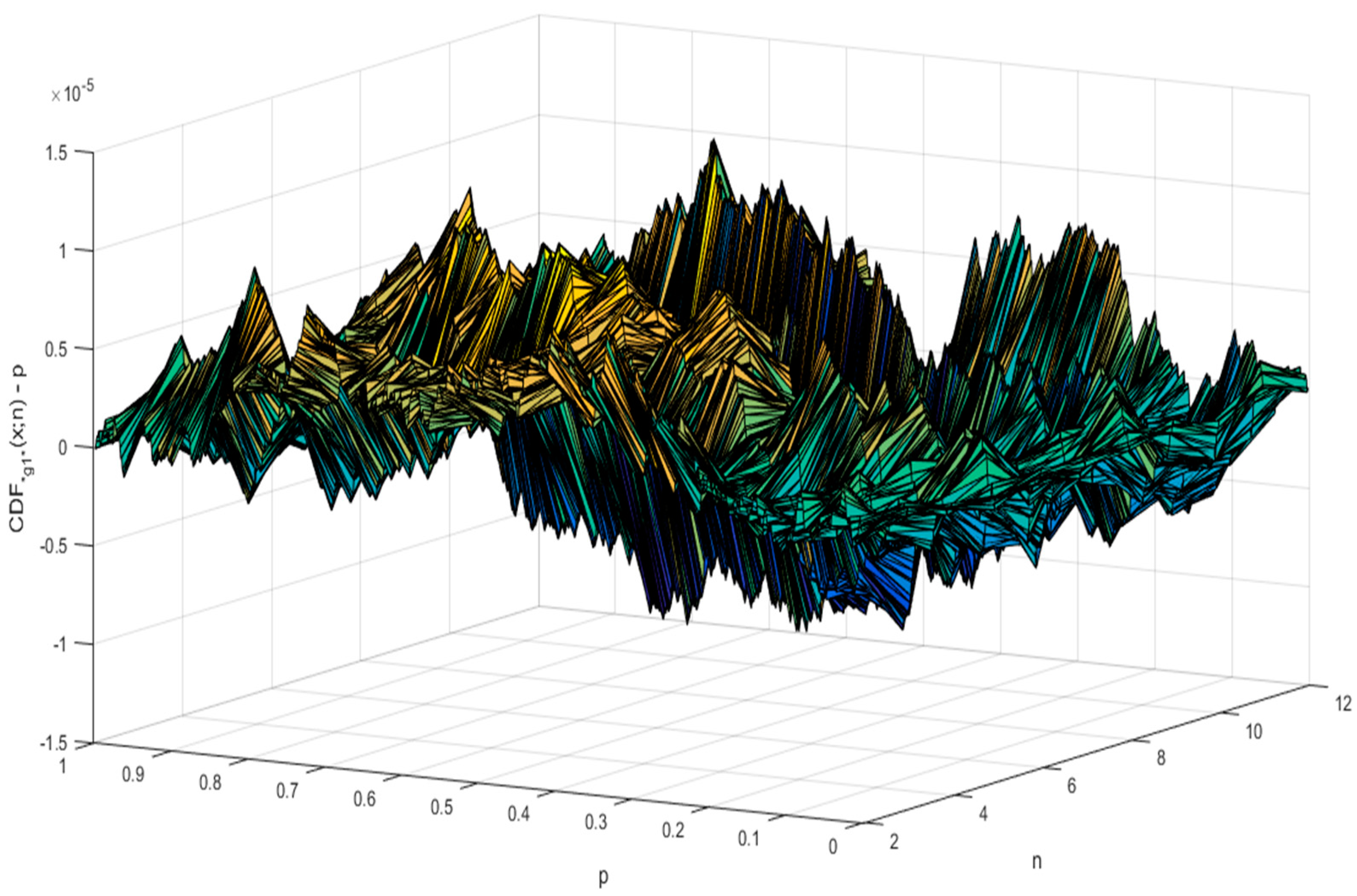
As can be observed in Table 3 the standard error (SE) slowly decreases beginning with n = 7, being two orders of magnitude smaller (actually it is about 200 times smaller) than the step from the MC experiment. Since the standard error alone is not proof that Equation (11) is the true CDF formula for providing the probability for the g1 statistic, the smallest and the highest difference between the observed and the expected probabilities are also given in Table 3. They substantiate that Equation (11) is indeed the right estimate for the CDF of g1. For convenience, Figure 1 shows the value of the error in each observation point (999 points corresponding to p = 0.001 up to p = 0.999 for each n from 2 to 12).

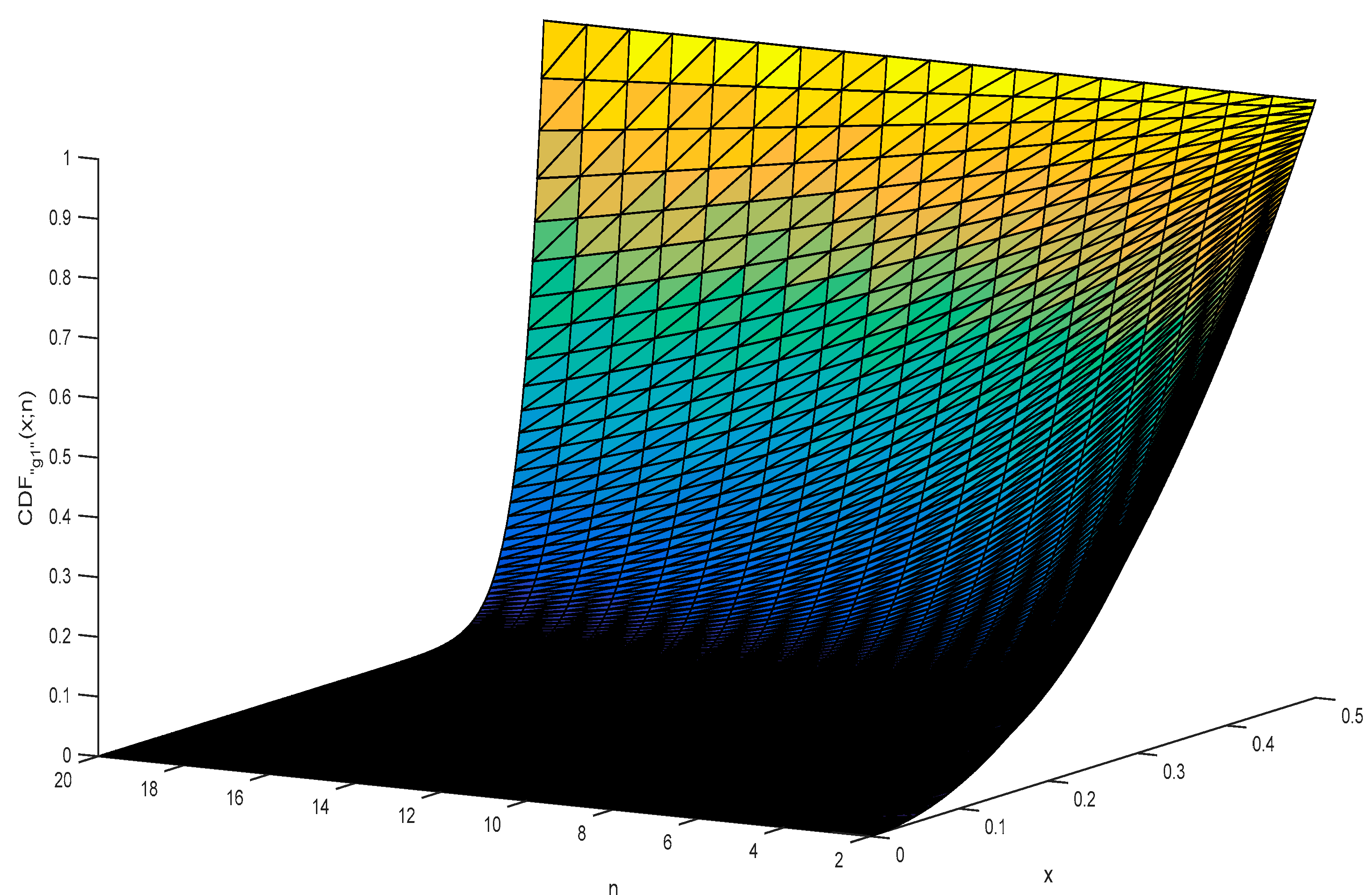
Regarding the estimation error (of the “g1” statistic) depicted in Figure 1, the “g1” statistic is rarely bigger than 10⁻⁵, never bigger than 1.5·× 10⁻⁵ and tends to become smaller with the increase in sample size (n). Using Equation (11), Figure 2 depicts the shape of the CDF_“g1”(x;n).

With regard to the “g1” statistic (depicted in Figure 2), the domain for a variable distributed by the “g1” statistic (see Equation (11)) has values between 0 and 0.5 with the mode at p = 0 (a vertical asymptote at p = 0), a median of n⁻¹·2^−1/n (and having a left asymmetry decreasing with the increasing of n and converging (for n → ∞) to symmetry) and mean of 1/2(n+1).

The expression of CDF_“g1” is easily inverted (see Equation (13)).

$${\mathrm{CDF}}_{“\mathrm{g}1”}(\mathrm{x};\mathrm{n})=(2\mathrm{x}{)}^{\mathrm{n}}\to {\mathrm{InvCDF}}_{“\mathrm{g}1”}(\mathrm{p};\mathrm{n})=\sqrt[n]{p}/2$$

(13)

7. from “g1” Statistic to “g1” Confidence Intervals for the Extreme Values

Equation (13) can be used to calculate the critical values of the “g1” statistic for any values of α (α ← 1-p) and n. The critical values of the “g1” statistic acts as the boundaries of the confidence intervals.

By setting the risk of being in error α (usually at 5%), then p = 1-α and Equation (13) can be used to calculate the statistic associated with it (InvCDF_“g1”(1-α;n) = $\sqrt[n]{1-\alpha }/2$). By placing this value into Equations (9) and (10), the (extreme) probabilities can be extracted (Equation (14)).

$$\underset{1\le i\le n}{\max }\left|p_i-0.5\right|=\sqrt[n]{1-\alpha }/2.\to {\mathrm{p}}_{\mathrm{extreme}}(\mathsf{\alpha })=0.5\pm \sqrt[n]{1-\alpha }/2$$

(14)

One should note that the confidence interval defined by Equation (14) is symmetric.

In order to arrive at the confidence intervals for the extreme values in the sampled data (Equation (15)) it is necessary to use the inverse of the CDF (again), and for the distribution of the sampled data.

$${\mathrm{x}}_{\mathrm{extreme}}(\mathsf{\alpha })={\mathrm{InvCDF}}_{“\mathrm{Distribution}”}(0.5\pm \sqrt[\mathrm{n}]{1-\mathsf{\alpha }}/2;“\mathrm{parameters}”)$$

(15)

To illustrate the calculation of the confidence intervals for the extreme values in the sampled data, a series of 206 data was chosen from [32]. The data were tested against the assumption that it follows a generalized Gauss-Laplace distribution (Equation (16), a symmetrical distribution), and later if there were some observations suspected to be outliers. The steps of this analysis and the obtained results are given in

Table 4. Distribution analysis for a series of 206 measurements for the octanol water partition coefficient (K_ow) of polychlorinated biphenyls expressed in logarithmic scale (log₁₀(K_ow))

Step	Results
Dataset (given for convenience)	4.151; 4.401; 4.421; 4.601; 4.941; 5.021; 5.023; 5.150; 5.180; 5.295; 5.301; 5.311; 5.311; 5.335; 5.343; 5.404; 5.421; 5.447; 5.452; 5.452; 5.481; 5.504; 5.517; 5.537; 5.537; 5.551; 5.561; 5.572; 5.577; 5.577; 5.627; 5.637; 5.637; 5.667; 5.667; 5.671; 5.677; 5.677; 5.691; 5.717; 5.743; 5.751; 5.757; 5.761; 5.767; 5.767; 5.787; 5.811; 5.817; 5.827; 5.867; 5.897; 5.897; 5.904; 5.943; 5.957; 5.957; 5.987; 6.041; 6.047; 6.047; 6.047; 6.057; 6.077; 6.091; 6.111; 6.117; 6.117; 6.137; 6.137; 6.137; 6.137; 6.137; 6.142; 6.167; 6.177; 6.177; 6.177; 6.204; 6.207; 6.221; 6.227; 6.227; 6.231; 6.237; 6.257; 6.267; 6.267; 6.267; 6.291; 6.304; 6.327; 6.357; 6.357; 6.367; 6.367; 6.371; 6.427; 6.457; 6.467; 6.487; 6.497; 6.511; 6.517; 6.517; 6.523; 6.532; 6.547; 6.583; 6.587; 6.587; 6.587; 6.607; 6.611; 6.647; 6.647; 6.647; 6.647; 6.647; 6.657; 6.657; 6.671; 6.671; 6.677; 6.677; 6.677; 6.697; 6.704; 6.717; 6.717; 6.737; 6.737; 6.737; 6.747; 6.767; 6.767; 6.767; 6.797; 6.827; 6.857; 6.867; 6.897; 6.897; 6.937; 6.937; 6.957; 6.961; 6.997; 7.027; 7.027; 7.027; 7.057; 7.071; 7.087; 7.087; 7.117; 7.117; 7.117; 7.121; 7.123; 7.147; 7.151; 7.177; 7.177; 7.187; 7.187; 7.207; 7.207; 7.207; 7.211; 7.247; 7.247; 7.277; 7.277; 7.277; 7.281; 7.304; 7.307; 7.307; 7.321; 7.337; 7.367; 7.391; 7.427; 7.441; 7.467; 7.516; 7.527; 7.527; 7.557; 7.567; 7.592; 7.627; 7.627; 7.657; 7.657; 7.717; 7.747; 7.751; 7.933; 8.007; 8.164; 8.423; 8.683; 9.143; 9.603
For n = 206 calculate the probability that the extreme values contain an outlier by using Equation (13)	At α = 5% risk being in error InvCDF“g1”(1-0.05; 206) = 0.498755
Calculate the critical probabilities for the extreme values by using Equations (9) and (10)	g1 = 0.498755 → |0.5 - pmin/max| = 0.498755 → 1 - 2pmin/max = ± 0.99751 → pmin = 0.0001245; pmax = 0.9998755
Estimate the parameters of the distribution fitting the dataset (distribution: Gauss-Laplace; μ - location parameter; σ - scale parameter; k - shape parameter)	Initial estimates (from a hybrid CM & MLE method): μ = 6.4806; σ = 0.83076; k = 1.4645; MLE estimates (by applying eq.3): μ = 6.47938; σ = 0.82828; k = 1.79106;
Calculate the lower and the upper bound for the extreme values by using InvCDF of the distribution fitting the data (Equation (15))	InvCDF“GL”(0.0001245; μ = 6.47938, σ = 0.82828, k = 1.79106) = 3.2409 InvCDF“GL”(0.9998755; μ = 6.47938, σ = 0.82828, k = 1.79106) = 9.7178
Make the conclusion regarding the outliers	Since the smallest value in the dataset is 4.151 (> 3.24) and the largest value is 9.603 (< 9.71), at 5% risk being in error there are no outliers in the dataset on the assumption that data follows the Gauss-Laplace distribution

.

$${\mathrm{PDF}}_{“\mathrm{GL}”}(\mathrm{x};\mathsf{\mu },\mathsf{\sigma },\mathrm{k})={\mathrm{c}}_1{\mathsf{\sigma }}^{-1}{\mathrm{e}}^{-{\left|{\mathrm{c}}_0\mathrm{z}\right|}^{\mathrm{k}}},{\mathrm{c}}_0={(\frac{\mathsf{\Gamma }(3/\mathrm{k})}{\mathsf{\Gamma }(1/\mathrm{k})})}^{1/2},{\mathrm{c}}_1=\frac{{\mathrm{kc}}_0}{2\mathsf{\Gamma }(1/\mathrm{k})},\mathrm{z}=\frac{\mathrm{x}-\mathsf{\mu }}{\mathsf{\sigma }}$$

(16)

The greatest departure from the median (0.5) for the 206 PCB dataset (Table 4) was 9.603 (CDF_“GL”(9.603; μ = 6.47938, σ = 0.82828, k = 1.79106) = 0.9998). Due to the force of this deviation from the median, 9.603 was suspected as being an outlier and was removed (it should be noted that in a broader context, an outlier can be also seen as an atypical observation, correctly collected from the population observation, as part of the data generation process and thus it may be maintained in the sample but probably with a less weight). The same procedure (as in Table 4) can be applied to the remaining data (205 observations). Then, InvCDF_“g1”(1-0.05; 205) = 0.499875, p_min(n=205) = 0.0001251; and p_max(n=205) = 0.9998749. The MLE estimates for the parameters of the Gauss-Laplace distribution remain unchanged (μ = 6.47938, σ = 0.82828, k = 1.79106) and the removed observation (9.603) is still not an outlier (x_max = InvCDF_“GL”(0.9998749; μ = 6.47938, σ = 0.82828, k = 1.79106) = 9.7166 > 9.603).

8. Proposed Procedure for Detecting the Outliers

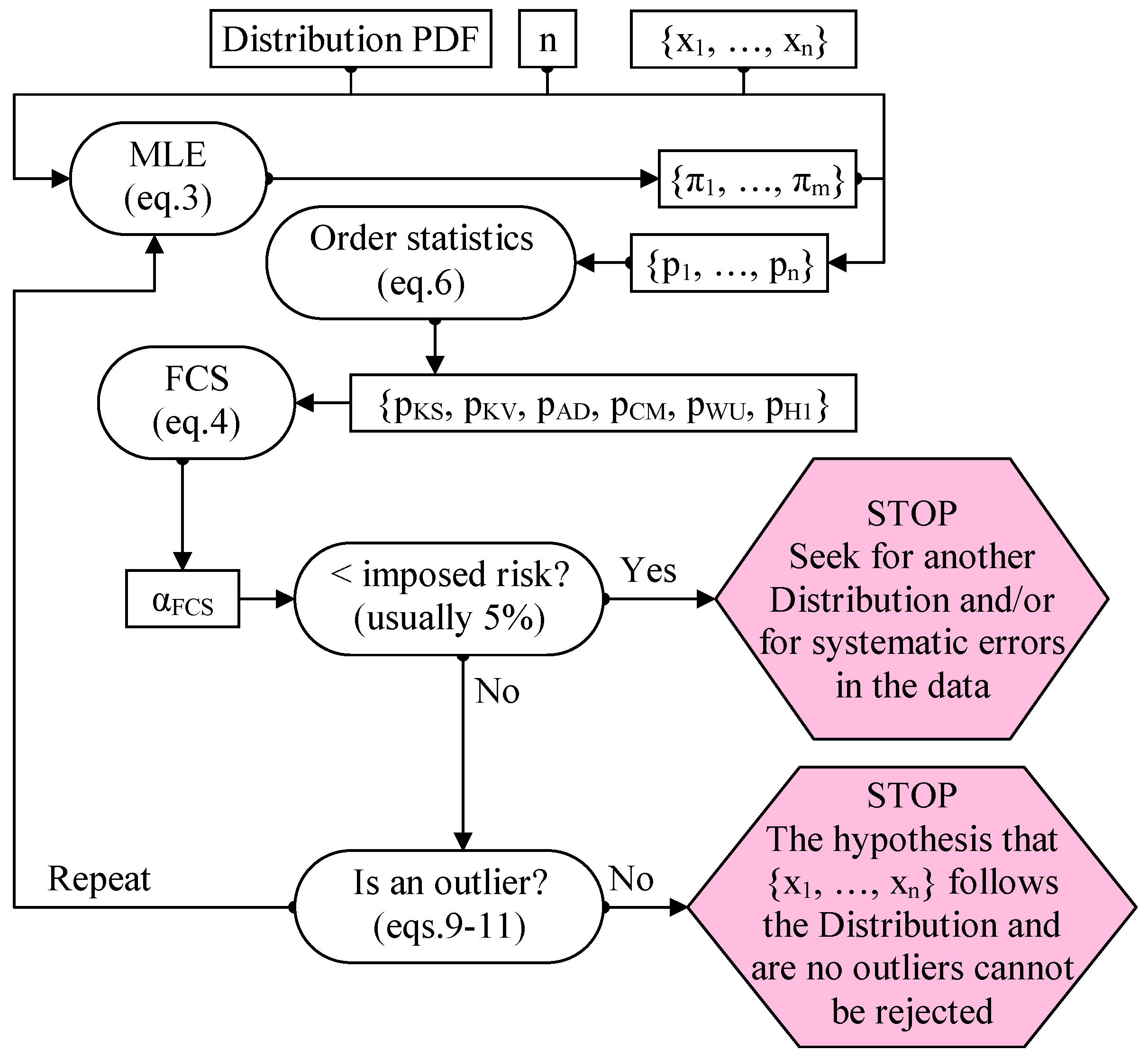
The procedure for detecting the outliers should start with measuring the agreement between the observed and estimated (Figure 3).

Figure 3 contains a statistical “trick”, namely, when there are no outliers the statistics measuring the gap between the observation and the model (order statistics, Equation (6)) are in agreement (their associated probabilities are not too far from each other). When outliers exist, the order statistics are also sensitive to their presence. Since this is a separate subject, for further discussion please see the series of papers beginning with [32,33,34].

9. Second Simulation Assessing “Grubbs” and “g1” Outlier Detection Alternatives

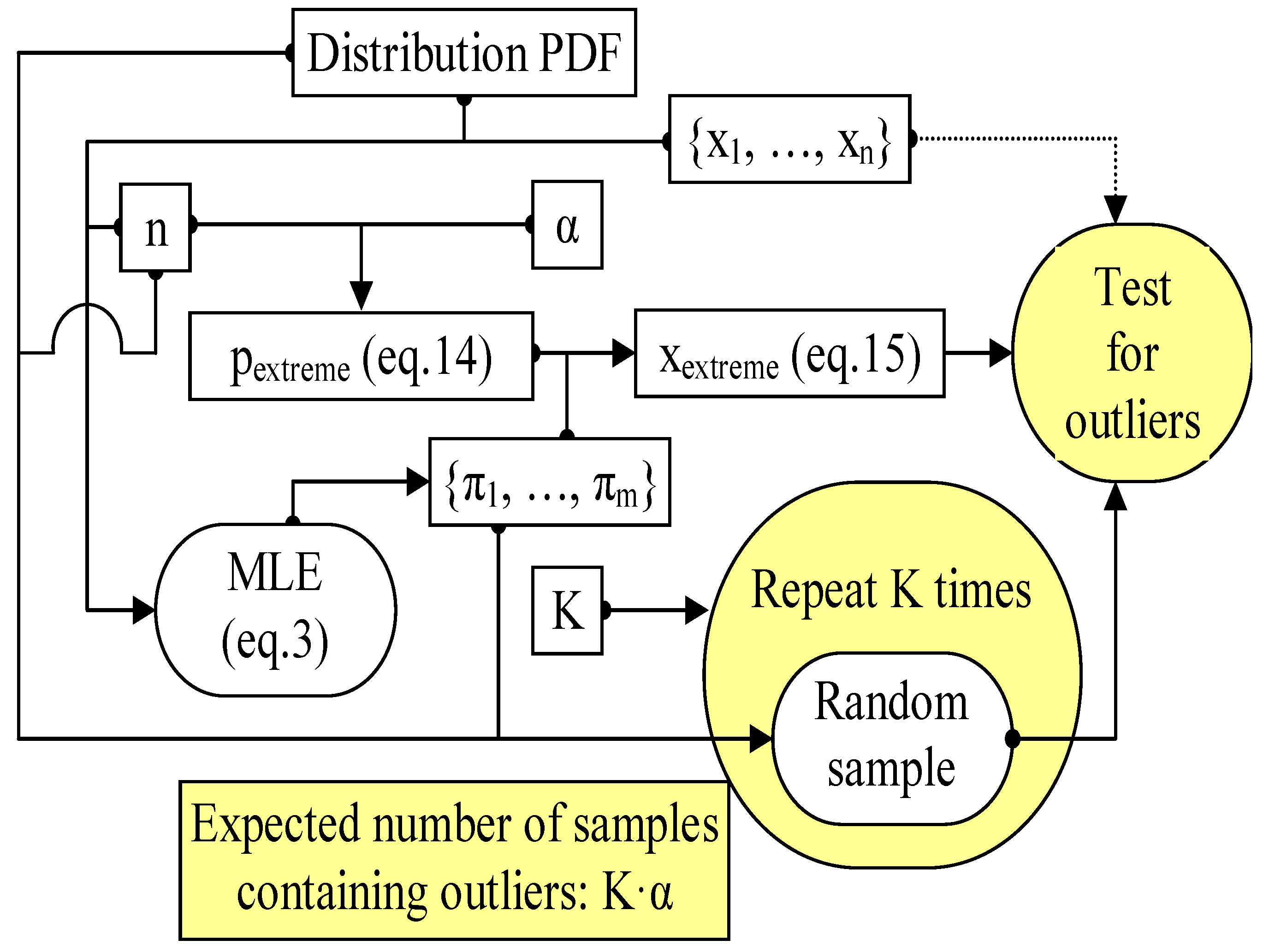
Another MC study was designed to test the claim that the proposed method provides consistent results. This second MC simulation is much simpler than the one used to derive the data for constructing the outlier statistics (Figure 4).

The data used here as a proof of the facts are from [7] and all cases involve a Normal distribution (Distribution = Normal in Equation (15); PDF and CDF for Normal distribution in Equation (18); a symmetrical distribution) with α = 5% risk being in error. The parameters of the Normal distribution (μ and σ) are determined for each case, as well as the sample size (Equation (17)).

$$x_{\mathrm{extreme}}(\alpha )={\mathrm{InvCDF}}_{“\mathrm{Normal}”}(0.5\pm 0.5·\sqrt[n]{1-\mathsf{\alpha }};\mu ,\sigma )$$

(17)

$${\mathrm{PDF}}_{“\mathrm{Normal}”}(x;\mu ,\sigma )=\frac{e^{-\frac{{(x-\mu )}^2}{{\sigma }^2}}}{\sigma \sqrt{2\pi }},{\mathrm{CDF}}_{“\mathrm{Normal}”}(x;\mu ,\sigma )={{\displaystyle \int }}_{-\infty }^x{\mathrm{PDF}}_{“\mathrm{Normal}”}(t;\mu ,\sigma )dt$$

(18)

For comparison, the same strategy for calculating the confidence intervals of the extreme values for the Normal distribution with the Grubbs test statistic (Equation (2)) was used to provide an alternate result (Equation (19)).

$$x_{\mathrm{crit}}(\alpha )=\overline{x}\pm G_{\mathrm{crit}}(\alpha )\cdot s,G_{\mathrm{crit}}(\alpha )=\frac{\mathrm{n}-1}{\sqrt{n}}\sqrt{\frac{t_G^2(\alpha )}{\mathrm{n}-2+t_G^2(\alpha )}},t_G={\mathrm{InvCDF}}_{“\mathrm{Student}\mathrm{t}”}(\frac{\alpha }{2n},\mathrm{n}-2)$$

(19)

The steps followed in this analysis are given in the

Table 5. Comparison of the steps of the analysis and simulation for extreme values confidence intervals (proposed method vs. Grubbs test)

Step	Action (step 0 is setting the dataset; α ← 0.05)
1	Estimate (with MLE, Equation (3)) parameters (μ, σ) of the Normal distribution; calculate the associated CDFs (Equation (18))
2	Calculate the order statistics, their associated risks being in error, FCS and pFCS (Equations (6) and (4))
3	For n and α calculate the confidence intervals for the extreme values by using (a) Equation (6) and (17) and (b) Equation (19)
4	Run the MC experiment (Figure 4) for K = 10000 (and then the expected number of outliers is 500) samples and count the samples containing outliers for the existing method (Grubbs, Equation (19); with μ and σ from CM method) and for the proposed method (g1, Equations (13)–(15) and (17); with μ and σ from the MLE method)

.

Results of the analysis using the steps given in Table 5 for the first dataset are given in

Table 6. Outlier analysis results for {568, 570, 570, 570, 572, 572, 572, 578, 584, 596} dataset.

Step	Results (for α = 5%)
1	μ = 575.2; σ = 8.256 (MLE) → CPs = {0.1916, 0.2644, 0.2644, 0.2644, 0.3492, 0.3492, 0.3492, 0.6328, 0.8568, 0.9941}
2		Statistic	AD	KS	CM	KV	WU	H1	FCS
		Value	1.137	1.110	0.206	1.715	0.182	5.266	12.293
		αStatistic	0.288	0.132	0.259	0.028	0.049	0.343	0.056
3	xcrit(5%) = 575.2 ± 2.29·8.7025; pextreme(5%) = 0.5 ± InvCDF“g1”(1-0.05; 10); xextreme(5%) = {552.086, 598.314}
4		Number of samples containing outliers			Existing method (Grubbs)		Proposed method (g1)
		First run			1977 (19.77%)		510 (5.1%)
		Second run			2009 (20.09%)		526 (5.26%)

.

In regard to the results given in Table 6:

At step 1, CPs are the cumulative probabilities ({p₁, …, p₁₀} in Figure 3) associated with the series of the observations from the sample ({x₁, …, x₁₀} in Figure 3).

At step 2, the data passes the normality test (α_FCS = 7% > 5% = α, see Figure 3).

Step 3 was made for n = 10 (see Figure 4). (a) The proposed method does not detect outliers in the sample (552.086 < 568, 596 < 598.314); (b) Grubbs test detect 596 as being an outlier (596 > 595.13).

At step 4 (see Figure 4), since {510, 526} are comparable with 500 and {1977, 2009} are much greater than 500, the results lead to the conclusion that the existing method produces type I errors by leading to false positive detection of outliers in the samples while the proposed method does not.

10. Going Further with the Outlier Analysis

What if “596” is removed from the sample? The following table provides mirror-like results for this scenario (

Table 7. Outlier analysis results for {568, 570, 570, 570, 572, 572, 572, 578, 584} dataset.

Step	Results (for α = 5%)
1	μ = 572.889; σ = 4.725 (MLE) → CPs = {0.1504, 0.2705, 0.2705, 0.2705, 0.4254, 0.4254, 0.4254, 0.8603, 0.9907}
2		Statistic	AD	KS	CM	KV	WU	H1	FCS
		Value	0.935	1.057	0.174	1.535	0.155	4.678	9.715
		αStatistic	0.389	0.167	0.327	0.082	0.088	0.394	0.137
3	xcrit(5%) = 572.89 ± 2.215·5.011; pextreme(5%) = 0.5 ± InvCDF“g1”(1-0.05; 9); xextreme(5%) = {559.822, 585.956}
4		Number of samples containing outliers			Existing method (Grubbs)		Proposed method (g1)
		First run			2341 (23.41%)		563 (5.63%)
		Second run			2333 (23.33%)		543 (5.43%)

).

As can be observed in Table 7, the data is not in good agreement with normality (α_FCS in Table 6 is 7%, while in Table 7 it is 16%) and there is no change in the accuracy of the classification ({563, 543} comparable with 500, {2341, 2333} is much greater than 500; the existing method produces type I errors by leading to false positive detection of outliers in the samples, while the proposed method does not). When comparing the results given in Table 6 with the results given in Table 7 it should be noted that both tests (Grubbs and the newly proposed g1) produce somewhat confusing results (see

Table 8. Side-by-side comparison of the analysis of the samples.

Sample	{568, 570, 570, 570, 572, 572, 572, 578, 584, 596}	{568, 570, 570, 570, 572, 572, 572, 578, 584}
At 5% risk being in error can the hypothesis that the sample was drawn from a normal distribution be rejected?	No (αFCS = 7%)	No (αFCS = 15.8%)
Grubbs confidence interval for ‘no outliers’ at 5% risk being in error	(555.27, 595.13) 596 is detected as being outlier	(561.79, 583.99) 584 is detected as being outlier
g1 confidence interval for ‘no outliers’ at 5% risk being in error	(552.08, 598.32) no outliers	(559.82, 585.96) no outliers

for side-by-side outcomes).

Table 8 highlights the fact that based on the {568, 570, 570, 570, 572, 572, 572, 578, 584} sample, the g1 test may be interpreted as identifying 596 as being an outlier. This is not quite true because the g1 test was not intended to be used in this way. That is, 596 is outside of the dataset, so at the time of constructing the confidence intervals for the extreme values, the information regarding its observation was missing.

Another trial was done, this time with 601 replacing 596 in the initial dataset (

Table 9. Outlier analysis results for the {568, 570, 570, 570, 572, 572, 572, 578, 584, 601} dataset.

Step	Results (for α = 5%)
1	From the CM method: μ = 575.7; σ = 10.067; from MLE method: μ = 575.7; σ = 9.550
2		Statistic	AD	KS	CM	KV	WU	H1	FCS
		Value	1.267	1.109	0.225	1.774	0.198	5.411	13.652
		αStatistic	0.241	0.132	0.226	0.018	0.035	0.254	0.034
3	Grubbs confidence interval for ’no outliers’ at 5% risk being in error: (552.647,598.753); 601 is an outlier g1 confidence interval for ’no outliers’ at 5% risk being in error: (548.963, 602.437); no outliers

).

In a further trial, 604 replaced 596 in the initial dataset (

Table 10. Outlier analysis results for the {568, 570, 570, 570, 572, 572, 572, 578, 584, 604} dataset.

Step	Results (for α = 5%)
1	From the CM method: μ = 576.0; σ = 10.914; from MLE method: μ = 576.0; σ = 10.354
2		Statistic	AD	KS	CM	KV	WU	H1	FCS
		Value	1.348	1.108	0.238	1.803	0.209	5.481	14.468
		αStatistic	0.216	0.133	0.206	0.015	0.028	0.215	0.025
3	Grubbs confidence interval for ’no outliers’ at 5% risk being in error: (551.00, 601.00); 604 is an outlier g1 confidence interval for ’no outliers’ at 5% risk being in error: (547.01, 604.99); no outliers

).

The conclusion is simple (see the results in the Table 6, Table 7, Table 9 and Table 10): A test will hardly ever detect an outlier for a small sample; it is more likely to reject the hypothesis of the sample drawn from the distribution itself!

The same trick was used on a bigger sample and the results are shown in

Table 11. Outlier analysis results for Table 4 dataset under the assumption of normal distribution.

Step	Results (for α = 5%)
1	Table 5 Dataset; Normal distribution → CM: μ = 6.481; σ = 0.831; MLE: μ = 6.481; σ = 0.829
2		Statistic	AD	KS	CM	KV	WU	H1	FCS
		Value	0.439	0.484	0.049	0.952	0.047	104.2	1.276
		αStatistic	0.812	0.965	0.886	0.852	0.743	0.641	0.973
3	Grubbs confidence interval for ’no outliers’ at 5% risk being in error: (3.492, 9.470); 9.603 is an outlier g1 confidence interval for ’no outliers’ at 5% risk being in error: (3.444, 9.517); 9.603 is an outlier
4		Number of samples containing outliers			Existing method (Grubbs)		Proposed method (g1)
		First run			637 (6.37%)		511 (5.11%)
		Second run			630 (6.3%)		481 (4.81%)

(the dataset is from Table 4).

On one hand, as the results in Table 11 prove, the proposed method correctly identifies the confidence interval for the extreme values, while the existing method does not.

On the other hand, the results in Table 11 also show that the likelihood of identifying the outliers increases with the sample size, making it perfectly possible to identify outliers with the proposed method, although this is not the case in small samples. It is possible to detect the outliers in small samples as well, but not when the parameters of the distribution are derived from the sample data—only when the parameters of the distribution are known a priori or determined from other samples (the results given in Table 6, Table 7, Table 8, Table 9 and Table 10 are proof of this).

11. Further Discussion

The obtained expression for CDF of “g1” (Equation (11)) reveals the domain of a random variable distributed by the “g1” statistic ([0, 0.5]), which is consistent with the definition of “g1” (Equations (9) and (10)).

Independently of the shape of the theoretical distribution being tested (the generic case is defined by Equation (5)), as defined by Equations (9) and (10), the newly proposed statistic “g1” defines a symmetric confidence interval for the extreme values in samples in the probability space (Equation (14)). Later, this symmetric confidence interval may be changed back into an asymmetrical one when it is expressed in the domain of the theoretical distribution being tested (Equation (15)). It should be recognized that “g1” uses a symmetrization strategy to obtain the confidence interval for the extreme values in samples.

It might seem that the literature on robust statistics was ignored in this work, however, this is not entirely true. In fact, a whole pool of robust statistics was used extensively in the study (see Equation (8)), introduced as a tool in Table 5 and involved in the later calculations (Table 6, Table 7 and Table 9, Table 10 and Table 11). Also, it should be noted that the substitution of the mean by the median is not a new idea; it is well known in the field of robust statistics (for example, Watson U² [29], the WU_Statistic in Equation (8), uses it).

A short literature survey provides several of examples of current real applications that require the proposed method. Thus, in signal processing, non-stationary, non-Gaussian, spiky signals are usually regarded as outliers and thus discarded (see [35,36,37,38] as typical cases). In this context, it should be noted that Mood’s median test is preferred to the Kruskal-Wallis test when outliers are present [39]. The identification of outliers is also recognized as an issue in the validation of protein structures, and the current methods are revised in [40]. Other examples can be found in [41].

In the wider context, an alternate window-based strategy has been proposed in which outliers are detected in each window by the Tukey method and labeled so that they can be excluded from the realization of the process points to be used for model identification [42]. A contingency-based strategy proposes maximization of true positive (TP) values and minimization of false negative (FN) and false positive (FP) values [43]. Finally, another distribution testing procedure has been proposed in [44].

12. Conclusions

A new method for detecting outliers was proposed in this paper. The method is applicable to any continuous distribution at any risk being in error. It was proved that the method correctly detects the outliers. For a normal distribution at 5% risk being in error, it was also shown that the proposed method outperforms the classical Grubbs test for detecting the outliers.

References

- Gauss, C.F. Theoria Motus Corporum Coelestium; (Translated in 1857 as “Theory of Motion of the Heavenly Bodies Moving about the Sun in Conic Sections” by C. H. Davis. Little, Brown: Boston. Reprinted in 1963 by Dover: New York); Perthes et Besser: Hamburg, Germany, 1809; pp. 249–259. [Google Scholar]
- Tippett, L.H.C. The extreme individuals and the range of samples taken from a normal population. Biometrika 1925, 17, 151–164. [Google Scholar] [CrossRef]
- Fisher, R.A.; Tippett, L.H.C. Limiting forms of the frequency distribution of the largest and smallest member of a sample. Proc. Camb. Philos. Soc. 1928, 24, 180–190. [Google Scholar] [CrossRef]
- Thompson, W.R. On a criterion for the rejection of observations and the distribution of the ratio of the deviation to the sample standard deviation. Ann. Math. Stat. 1935, 6, 214–219. [Google Scholar] [CrossRef]
- Pearson, E.; Sekar, C.C. The efficiency of the statistical tools and a criterion for the rejection of outlying observations. Biometrika 1936, 28, 308–320. [Google Scholar] [CrossRef]
- Grubbs, F.E. Sample criteria for testing outlying observations. Ann. Math. Stat. 1950, 21, 27–58. [Google Scholar] [CrossRef]
- Grubbs, F.E. Procedures for detecting outlying observations in samples. Technometrics 1969, 11, 1–21. [Google Scholar] [CrossRef]
- Nooghabi, M.; Nooghabi, H.; Nasiri, P. Detecting outliers in gamma distribution. Commun. Stat. Theory Methods 2010, 39, 698–706. [Google Scholar] [CrossRef]
- Kumar, N.; Lalitha, S. Testing for upper outliers in gamma sample. Commun. Stat. Theory Methods 2012, 41, 820–828. [Google Scholar] [CrossRef]
- Lucini, M.; Frery, A. Comments on “Detecting Outliers in Gamma Distribution” by M. Jabbari Nooghabi et al. (2010). Commun. Stat. Theory Methods 2017, 46, 5223–5227. [Google Scholar] [CrossRef]
- Hartley, H. The range in random samples. Biometrika 1942, 32, 334–348. [Google Scholar] [CrossRef]
- Bardet, J.-M.; Dimby, S.-F. A new non-parametric detector of univariate outliers for distributions with unbounded support. Extremes 2017, 20, 751–775. [Google Scholar] [CrossRef] [Green Version]
- Gosset, W. The probable error of a mean. Biometrika 1908, 6, 1–25. [Google Scholar]
- Jäntschi, L.; Bolboacă, S.-D. Computation of probability associated with Anderson-Darling statistic. Mathematics 2018, 6, 88. [Google Scholar] [CrossRef]
- Fisher, R. On an Absolute Criterion for Fitting Frequency Curves. Messenger Math. 1912, 41, 155–160. [Google Scholar]
- Fisher, R. Questions and answers #14. Am. Stat. 1948, 2, 30–31. [Google Scholar]
- Bolboacă, S.D.; Jäntschi, L.; Sestraș, A.F.; Sestraș, R.E.; Pamfil, D.C. Supplementary material of ’Pearson-Fisher chi-square statistic revisited’. Information 2011, 2, 528–545. [Google Scholar] [CrossRef]
- Jäntschi, L.; Bolboacă, S.D. Performances of Shannon’s Entropy Statistic in Assessment of Distribution of Data. Ovidius Univ. Ann. Chem. 2017, 28, 30–42. [Google Scholar] [CrossRef]
- Davis, P.; Rabinowitz, P. Methods of Numerical Integration; Academic Press: New York, NY, USA, 1975; pp. 51–198. [Google Scholar]
- Pearson, K. Note on Francis Gallon’s problem. Biometrika 1902, 1, 390–399. [Google Scholar]
- Cramér, H. On the composition of elementary errors. Scand. Actuar. J. 1928, 1, 13–74. [Google Scholar] [CrossRef]
- Von Mises, R.E. Wahrscheinlichkeit, Statistik und Wahrheit; Julius Springer: Berlin, Germany, 1928; pp. 100–138. [Google Scholar]
- Kolmogorov, A. Sulla determinazione empirica di una legge di distribuzione. Giornale dell’Istituto Italiano degli Attuari 1933, 4, 83–91. [Google Scholar]
- Kolmogorov, A. Confidence Limits for an Unknown Distribution Function. Ann. Math. Stat. 1941, 12, 461–463. [Google Scholar] [CrossRef]
- Smirnov, N. Table for estimating the goodness of fit of empirical distributions. Ann. Math. Stat. 1948, 19, 279–281. [Google Scholar] [CrossRef]
- Anderson, T.W.; Darling, D.A. Asymptotic theory of certain “goodness-of-fit” criteria based on stochastic processes. Ann. Math. Stat. 1952, 23, 193–212. [Google Scholar] [CrossRef]
- Anderson, T.W.; Darling, D.A. A Test of Goodness-of-Fit. J. Am. Stat. Assoc. 1954, 49, 765–769. [Google Scholar] [CrossRef]
- Kuiper, N.H. Tests concerning random points on a circle. Proc. Koninklijke Nederlandse Akademie van Wetenschappen Series A 1960, 63, 38–47. [Google Scholar] [CrossRef] [Green Version]
- Watson, G.S. Goodness-Of-Fit Tests on a Circle. Biometrika 1961, 48, 109–114. [Google Scholar] [CrossRef]
- Metropolis, N.; Ulam, S. The Monte Carlo Method. J. Am. Stat. Assoc. 1949, 44, 335–341. [Google Scholar] [CrossRef] [PubMed]
- Fisher, R.A. On the mathematical foundations of theoretical statistics. Philos. Trans. R. Soc. A 1922, 222, 309–368. [Google Scholar] [CrossRef] [Green Version]
- Jäntschi, L. Distribution fitting 1. Parameters estimation under assumption of agreement between observation and model. Bull. UASVM Hortic. 2009, 66, 684–690. [Google Scholar]
- Jäntschi, L.; Bolboacă, S.D. Distribution fitting 2. Pearson-Fisher, Kolmogorov-Smirnov, Anderson-Darling, Wilks-Shapiro, Kramer-von-Misses and Jarque-Bera statistics. Bull. UASVM Hortic. 2009, 66, 691–697. [Google Scholar]
- Bolboacă, S.D.; Jäntschi, L. Distribution fitting 3. Analysis under normality assumption. Bull. UASVM Hortic. 2009, 66, 698–705. [Google Scholar]
- Liu, K.; Chen, Y.Q.; Domański, P.D.; Zhang, X. A novel method for control performance assessment with fractional order signal processing and its application to semiconductor manufacturing. Algorithms 2018, 11, 90. [Google Scholar] [CrossRef]
- Paiva, J.S.; Ribeiro, R.S.R.; Cunha, J.P.S.; Rosa, C.C.; Jorge, P.A.S. Single particle differentiation through 2D optical fiber trapping and back-scattered signal statistical analysis: An exploratory approach. Sensors 2018, 18, 710. [Google Scholar] [CrossRef] [PubMed]
- Teunissen, P.J.G.; Imparato, D.; Tiberius, C.C.J.M. Does RAIM with correct exclusion produce unbiased positions? Sensors 2017, 17, 1508. [Google Scholar] [CrossRef] [PubMed]
- Pan, Z.; Liu, L.; Qiu, X.; Lei, B. Fast vessel detection in Gaofen-3 SAR images with ultrafine strip-map mode. Sensors 2017, 17, 1578. [Google Scholar] [CrossRef] [PubMed]
- Vergura, S.; Carpentieri, M. Statistics to detect low-intensity anomalies in PV systems. Energies 2018, 11, 30. [Google Scholar] [CrossRef]
- Chen, L.; He, J.; Sazzed, S.; Walker, R. An investigation of atomic structures derived from X-ray crystallography and cryo-electron microscopy using distal blocks of side-chains. Molecules 2018, 23, 610. [Google Scholar] [CrossRef] [PubMed]
- Bolboacă, S.D.; Jäntschi, L. The effect of leverage and influential on structure-activity relationships. Comb. Chem. High Throughput Screen. 2013, 16, 288–297. [Google Scholar] [CrossRef] [PubMed]
- Faes, L.; Porta, A.; Nollo, G.; Javorka, M. Information decomposition in multivariate systems: Definitions, implementation and application to cardiovascular networks. Entropy 2017, 19, 5. [Google Scholar] [CrossRef]
- Li, G.; Wang, J.; Liang, J.; Yue, C. Application of sliding nest window control chart in data stream anomaly detection. Symmetry 2018, 10, 113. [Google Scholar] [CrossRef]
- Paolella, M.S. Stable-GARCH models for financial returns: Fast estimation and tests for stability. Econometrics 2016, 4, 25. [Google Scholar] [CrossRef]
Figure 1.
Departures between expected and observed probabilities for g1 statistic (Equation (10) vs. Equation (11)).
Figure 2.
CDF“g1”(x;n) for n = 2 to n = 20.
Figure 3.
The procedure for detecting outliers.
Figure 4.
The procedure for testing the outlier statistics.