Transformation Properties under the Operations of the Molecular Symmetry Groups G₃₆ and G₃₆(EM) of Ethane H₃CCH₃

Abstract

In the present work, we report a detailed description of the symmetry properties of the eight-atomic molecule ethane, with the aim of facilitating the variational calculations of rotation-vibration spectra of ethane and related molecules. Ethane consists of two methyl groups CH${}_3$ where the internal rotation (torsion) of one CH${}_3$ group relative to the other is of large amplitude and involves tunnelling between multiple minima of the potential energy function. The molecular symmetry group of ethane is the 36-element group G${}_{36}$, but the construction of symmetrised basis functions is most conveniently done in terms of the 72-element extended molecular symmetry group G${}_{36}$(EM). This group can subsequently be used in the construction of block-diagonal matrix representations of the ro-vibrational Hamiltonian for ethane. The derived transformation matrices associated with G${}_{36}$(EM) have been implemented in the variational nuclear motion program TROVE (Theoretical ROVibrational Energies). TROVE variational calculations are used as a practical example of a G${}_{36}$(EM) symmetry adaptation for large systems with a non-rigid, torsional degree of freedom. We present the derivation of irreducible transformation matrices for all 36 (72) operations of G${}_{36}$(M) (G${}_{36}$(EM)) and also describe algorithms for a numerical construction of these matrices based on a set of four (five) generators. The methodology presented is illustrated on the construction of the symmetry-adapted representations both of the potential energy function of ethane and of the rotation, torsion and vibration basis set functions.

1. Introduction

In variational calculations of molecular rotation-vibration energies and wavefunctions, a matrix representation of the molecular rotation-vibration Hamiltonian, constructed in terms of suitable basis functions, is diagonalised numerically. It is well known that this type of calculation can be facilitated by the introduction of symmetrised basis functions, i.e., basis functions that generate irreducible representations of a symmetry group for the molecule in question (see, for example, [1]). Even though the calculation of energies and wavefunctions can, in principle, be carried out without the use of symmetry, the subsequent simulation of molecular spectra, involving the computation of transition intensities, would be impossible in practice without the consideration of symmetry [2]. We implement the symmetry information in the variational calculation by defining groups of matrices that are isomorphic or homomorphic to the original symmetry group of the molecule and that are associated with the various irreducible representations (irreps) of this symmetry group [1]. When suitable matrix group elements are known, projection operator techniques are employed to obtain the desired symmetrised basis functions for the variational calculation [1]. In a recent paper [2], we described an example of such a symmetry adaption, in that we presented character tables and irreducible representation transformation matrices for D${}_{n\mathrm{h}}$ groups with arbitrary n-values. With these results, we could practically utilise the linear-molecule symmetry properties described by the D${}_{\infty \mathrm{h}}$ point group in numerical calculations with the variational nuclear motion program TROVE [3], the acetylene molecule ${}^{12}$C${}_2$H${}_2$ serving as an example. In the present work, we report an analogous analysis for the molecular symmetry (MS) group G${}_{36}$ and the extended molecular symmetry (EMS) group G${}_{36}$(EM) [1] of the ethane molecule H${}_3$${}^{12}$C${}^{12}$CH${}_3$, shown in Figure 1, with the aim of facilitating the solution of the rotation-vibration Schrödinger equation for ethane and related molecules.

The MS group G${}_{36}$ has been the subject of a number of studies (see, for example, [4,5]). The EMS group G${}_{36}$(EM) was studied in detail by Di Lauro and Lattanzi [6,7]. Examples of the application of the G${}_{36}$(EM) group include studies of the rotation-torsional spectra of various ethane-type molecules [8,9,10,11,12]. TROVE (Theoretical ROVibrational Energies) [3,13] is a general variational program for computing ro-vibrational spectra and properties for small- to medium-sized polyatomic molecules of arbitrary structure. It has been applied to a large number of polyatomic species [13,14,15,16,17,18,19,20,21,22,23,24,25,26,27,28,29,30,31,32,33], most of which have considerable symmetry (e.g., with molecular symmetry groups [1] such as C${}_{3\mathrm{v}}$(M), D${}_{n\mathrm{h}}$(M) and T${}_{\mathrm{d}}$(M)). TROVE is an efficient computer program for simulating hot spectra of polyatomic molecules; it is one of the main tools of the ExoMol project [34,35]. The most recent updates of TROVE have been reported in Refs. [35,36]. TROVE uses an automatic approach for constructing a symmetry-adapted basis set to be used in setting up a matrix representation of the molecular rotation-vibration Hamiltonian. As mentioned above, we require towards this end, for each irrep of the symmetry group in question [1], a group of matrices constituting that irrep. However, for G${}_{36}$ or G${}_{36}$(EM), these matrices have not been available in the literature thus far. The present work aims at describing fully the groups G${}_{36}$ and G${}_{36}$(EM) and, in particular, determining matrix groups that define the irreps. The matrix groups obtained are used for symmetrising the potential energy surface and the rotation-vibration basis functions for ethane.

2. The Structure of the G₃₆ Group

Longuet-Higgins [37] showed that the group G${}_{36}$ can be written as a direct product of two smaller groups C${}_{3\mathrm{v}}^{(-)}$ and C${}_{3\mathrm{v}}^{(+)}$

$${\mathit{G}}_{36}={\mathit{C}}_{3\mathrm{v}}^{(-)}\times {\mathit{C}}_{3\mathrm{v}}^{(+)};$$

(1)

both of these groups are of order 6 and isomorphic to the C${}_{3\mathrm{v}}$ point group. The top row and leftmost column of

Table 1. The class structure of G${}_{36}$${}^a$.

${\mathit{R}}_1^{(-)}$ = ${\mathit{R}}_1^{(+)}$ = E	${\mathit{R}}_2^{(-)}$ = (132)(456)	${\mathit{R}}_3^{(-)}$ = (123)(465)	${\mathit{R}}_4^{(-)}$ = (14)(25)(36)($\mathit{ab}$)	${\mathit{R}}_5^{(-)}$ = (16)(24)(35)($\mathit{ab}$)	${\mathit{R}}_6^{(-)}$ = (15)(26)(34)($\mathit{ab}$)
$R_2^{(+)}$ = $\left(123\right)\left(456\right)$	$\left(465\right)$	$\left(132\right)$	$\left(153426\right)\left(ab\right)$	$\left(143625\right)\left(ab\right)$	$\left(163524\right)\left(ab\right)$
$R_3^{(+)}$ = (132)(465)	(123)	(456)	(162435)$\left(ab\right)$	(152634)$\left(ab\right)$	(142536)$\left(ab\right)$
$R_4^{(+)}$ = (14)(26)(35)${\left(ab\right)}^{*}$	(152436)${\left(ab\right)}^{*}$	(163425)${\left(ab\right)}^{*}$	(23)(56)${}^{*}$	(12)(46)${}^{*}$	(13)(45)${}^{*}$
$R_5^{(+)}$ = (16)(25)(34)${\left(ab\right)}^{*}$	$\left(142635\right){\left(ab\right)}^{*}$	$\left(153624\right){\left(ab\right)}^{*}$	(13)(46)${}^{*}$	(23)(45)${}^{*}$	(12)(56)${}^{*}$
$R_6^{(+)}$ = (15)(24)(36)${\left(ab\right)}^{*}$	(162534)${\left(ab\right)}^{*}$	(143526)${\left(ab\right)}^{*}$	(12)(45)${}^{*}$	(13)(56)${}^{*}$	(23)(46)${}^{*}$

${}^a$ The top row and leftmost column contain the G${}_{36}$ elements that also belong to the C${}_{3\mathrm{v}}^{(-)}$ or C${}_{3\mathrm{v}}^{(+)}$ group, respectively. The remaining entries are the products $R_j^{(-)}{R}_k^{(+)}$ = $R_k^{(+)}{R}_j^{(-)}$, where $R_j^{(-)}$ ∈ C${}_{3\mathrm{v}}^{(-)}$ is at the top of the column and $R_k^{(+)}$ ∈ C${}_{3\mathrm{v}}^{(+)}$ is at the left end of the row. The horizontal and vertical lines denote the separation of the classes.

define the elements of these two groups. For convenience, we label the elements of C${}_{3\mathrm{v}}^{(\pm )}$ as $R_j^{(\pm )}$, j = 1, 2, …, 6; this notation is also defined in Table 1. The nuclei are labelled as in Figure 2.

In Table 1, we list the products $R_j^{(-)}{R}_k^{(+)}$ = $R_k^{(+)}{R}_j^{(-)}$, where $R_j^{(-)}$ ∈ C${}_{3\mathrm{v}}^{(-)}$ and $R_k^{(+)}$ ∈ C${}_{3\mathrm{v}}^{(+)}$. Since G${}_{36}$ = C${}_{3\mathrm{v}}^{(-)}$ × C${}_{3\mathrm{v}}^{(+)}$, the 36 possible products $R_j^{(-)}{R}_k^{(+)}$ = $R_k^{(+)}{R}_j^{(-)}$ constitute the complete group G${}_{36}$.

Each of the groups C${}_{3\mathrm{v}}^{(-)}$ and C${}_{3\mathrm{v}}^{(+)}$ has three classes, ${\mathcal{C}}_1^{(\pm )}$ = $\{E\}$ = $\{R_1^{(\pm )}\}$, ${\mathcal{C}}_2^{(\pm )}$ = $\{R_2^{(\pm )},R_3^{(\pm )}\}$, and ${\mathcal{C}}_3^{(\pm )}$ = $\{R_4^{(\pm )},R_5^{(\pm )},R_6^{(\pm )}\}$. Since G${}_{36}$ is the direct product of C${}_{3\mathrm{v}}^{(-)}$ and C${}_{3\mathrm{v}}^{(+)}$ (where, as discussed by Longuet-Higgins [37], each element of C${}_{3\mathrm{v}}^{(-)}$ commutes with each element of C${}_{3\mathrm{v}}^{(+)}$), its classes are obtained as ${\mathcal{C}}_i^{(-)}\times {\mathcal{C}}_j^{(+)}$, that is, a class of G${}_{36}$ contains all elements $RS$ where R∈${\mathcal{C}}_i^{(-)}$ and S∈${\mathcal{C}}_j^{(+)}$. In the top row and leftmost column of Table 1, we indicate the class structures of C${}_{3\mathrm{v}}^{(+)}$ and C${}_{3\mathrm{v}}^{(-)}$, respectively. A class ${\mathcal{C}}_i^{(+)}$ of C${}_{3\mathrm{v}}^{(+)}$ is simultaneously, in the form ${\mathcal{C}}_1^{(-)}\times {\mathcal{C}}_i^{(+)}$, a class of G${}_{36}$. Similarly, the classes of C${}_{3\mathrm{v}}^{(-)}$ are simultaneously classes of G${}_{36}$. In Table 1, we indicate the complete set of G${}_{36}$ classes ${\mathcal{C}}_i^{(-)}\times {\mathcal{C}}_j^{(+)}$.

3. Irreducible Representations of G₃₆

Again, since G${}_{36}$ is the direct product of C${}_{3\mathrm{v}}^{(-)}$ and C${}_{3\mathrm{v}}^{(+)}$, we could in principle label its irreps as $({\Gamma }^{(-)},{\Gamma }^{(+)})$, where ${\Gamma }^{(-)}$ is an irrep of C${}_{3\mathrm{v}}^{(-)}$ and ${\Gamma }^{(+)}$ is an irrep of C${}_{3\mathrm{v}}^{(+)}$. C${}_{3\mathrm{v}}^{(-)}$ and C${}_{3\mathrm{v}}^{(+)}$ both have the one-dimensional irreps $A_1$ and $A_2$ together with the two-dimensional irrep E (

Table A1. Common character tables of C${}_{3\mathrm{v}}^{(-)}$ and C${}_{3\mathrm{v}}^{(+)}$.

$\mathbf{\Gamma }$	${\mathcal{C}}_1^{(\pm )}$	${\mathcal{C}}_2^{(\pm )}$	${\mathcal{C}}_3^{(\pm )}$
	1	2	3
$A_1$	1	1	1
$A_2$	1	1	−1
E	2	−1	0

in Appendix A). Customarily, the irreps of G${}_{36}$ are labelled as in Table 12 of Longuet-Higgins [37].

Table 2. Character table of G${}_{36}$.

${\mathbf{\Gamma }}_{36}$	$({\mathbf{\Gamma }}^{(-)},{\mathbf{\Gamma }}^{(+)})$	E	(123)(456)	(14)(26)(35)($\mathit{ab}$)${}^{*}$	(123)(465)	(123)	(142635)($\mathit{ab}$)${}^{*}$	(14)(25)(36)($\mathit{ab}$)	(142536)($\mathit{ab}$)	(12)(45)${}^{*}$
		1	2	3	2	4	6	3	6	9
$A_1$	$(A_1,A_1)$	1	1	1	1	1	1	1	1	1
$A_2$	$(A_2,A_1)$	1	1	1	1	1	1	−1	−1	−1
$A_3$	$(A_1,A_2)$	1	1	−1	1	1	−1	1	1	−1
$A_4$	$(A_2,A_2)$	1	1	−1	1	1	−1	−1	−1	1
$E_1$	$(E,A_1)$	2	2	2	−1	−1	−1	0	0	0
$E_2$	$(E,A_2)$	2	2	−2	−1	−1	1	0	0	0
$E_3$	$(A_1,E)$	2	−1	0	2	−1	0	2	−1	0
$E_4$	$(A_2,E)$	2	−1	0	2	−1	0	−2	1	0
G	$(E,E)$	4	−2	0	−2	1	0	0	0	0
		${\mathcal{C}}_1^{(-)}\times {\mathcal{C}}_1^{(+)}$	${\mathcal{C}}_1^{(-)}\times {\mathcal{C}}_2^{(+)}$	${\mathcal{C}}_1^{(-)}\times {\mathcal{C}}_3^{(+)}$	${\mathcal{C}}_2^{(-)}\times {\mathcal{C}}_1^{(+)}$	${\mathcal{C}}_2^{(-)}\times {\mathcal{C}}_2^{(+)}$	${\mathcal{C}}_2^{(-)}\times {\mathcal{C}}_3^{(+)}$	${\mathcal{C}}_3^{(-)}\times {\mathcal{C}}_1^{(+)}$	${\mathcal{C}}_3^{(-)}\times {\mathcal{C}}_2^{(+)}$	${\mathcal{C}}_3^{(-)}\times {\mathcal{C}}_3^{(+)}$

is the character table for G${}_{36}$, obtained from Table 12 of Longuet-Higgins [37], with the irreducible representations labelled by their customary labels ${\Gamma }_{36}$ and the combination labels $({\Gamma }^{(-)},{\Gamma }^{(+)})$. In the bottom row of the table, we indicate the ${\mathcal{C}}_i^{(-)}\times {\mathcal{C}}_j^{(+)}$ label of each class. For each of the nine G${}_{36}$ classes, we give in Table 2 a representative element together with the number of group elements in the class. The complete classes are obtained from Table 1.

In the present work, we are particularly concerned with the doubly-degenerate irreducible representations $E_1$ = $(E,A_1)$, $E_2$ = $(E,A_2)$, $E_3$ = $(A_1,E)$, and $E_4$ = $(A_2,E)$ together with the four-dimensional irreducible representation G = $(E,E)$.

In Section 12.4 of Ref. [1], and in Section 3.1 of Ref. [2], it is discussed how the point group C${}_{3\mathrm{v}}$ and any group isomorphic to it can be defined in terms of two generating operations, one of which belongs to the two-member class ${\mathcal{C}}_2^{(\pm )}$ of C${}_{3\mathrm{v}}$ and the other to the three-member class ${\mathcal{C}}_3^{(\pm )}$. For the group C${}_{3\mathrm{v}}^{(-)}$, we choose the generating operations as $R_2^{(-)}$ = (123)(465) and $R_4^{(-)}$ = (14)(25)(36)($ab$), whereas for C${}_{3\mathrm{v}}^{(+)}$, we choose $R_2^{(+)}$ = (123)(456) and $R_4^{(+)}$ = (14)(26)(35)($ab$)${}^{*}$. We then have $R_3^{(\pm )}={(R_2^{(\pm )})}^2$, $R_6^{(\pm )}=R_2^{(\pm )}{R}_4^{(\pm )}$, and $R_5^{(\pm )}=R_2^{(\pm )}{R}_6^{(\pm )}.$

4. Representation Matrices for the ${\mathit{E}}_{\mathit{i}}$ Irreducible Representations of G${}_{\mathbf{36}}$

The representation matrices for the non-degenerate irreps $A_1$, $A_2$, $A_3$, and $A_4$ of G${}_{36}$ are uniquely defined as equal to the representation characters; these can be found in Table 2. The $2\times 2$ representation matrices of the irreps $E_1$, $E_2$, $E_3$, and $E_4$ are, however, not uniquely defined. Having found one such set of matrices ${\mathbf{M}}_{E_i}\left[O_i\right]$, where $O_i$ ∈ G${}_{36}$, we can generate infinitely many equivalent representations with representation matrices ${\mathbf{M}}_{E_i}^{\prime }\left[O_i\right]$ = $\mathbf{V}{\mathbf{M}}_{E_i}\left[O_i\right]{\mathbf{V}}^{-1}$, where $\mathbf{V}$ is an arbitrary and invertible $2\times 2$ matrix. In practice, we want to keep the representation matrices real and orthogonal, and that drastically limits the possible choices. We select one particular set of representation matrices here for $E_1$ by initially choosing the representation matrix for $R_2^{(-)}$ = (123)(465), one of the generating operations of C${}_{3\mathrm{v}}^{(-)}$. We set

$${\mathbf{M}}_E\left[\left(123\right)\left(465\right)\right]=\left(\begin{array}{cc}cos\left(\frac{2\pi }{3}\right)& -sin\left(\frac{2\pi }{3}\right)\\ sin\left(\frac{2\pi }{3}\right)& cos\left(\frac{2\pi }{3}\right)\end{array}\right)=\left(\begin{array}{cc}-\frac{1}{2}& -\frac{\sqrt{3}}{2}\\ \frac{\sqrt{3}}{2}& -\frac{1}{2}\end{array}\right).$$

(2)

The $2\times 2$ orthogonal matrix ${\mathbf{M}}_E\left[\left(123\right)\left(465\right)\right]$ satisfies the relation ${\mathbf{M}}_E{\left[\left(123\right)\left(465\right)\right]}^3$ = $\mathbf{E}$, the $2\times 2$ unit matrix, imposed by the fact that ${\left[\left(123\right)\left(465\right)\right]}^3$ = E. An alternative choice would be the matrix with the signs of the $sin(2\pi /3)$ terms reversed. The other generating operation of C${}_{3\mathrm{v}}^{(-)}$, $R_4^{(-)}$ = [(14)(25)(36)($ab$)], is self-inverse: ${(R_4^{(-)})}^2$ = [(14)(25)(36)($ab$)]${}^2$ = E. The $2\times 2$ orthogonal matrix representing $R_4^{(-)}$ is also self-inverse and we can choose it as

$${\mathbf{M}}_E\left[\left(14\right)\left(25\right)\left(36\right)\left(ab\right)\right]=\left(\begin{array}{cc}cos\theta & sin\theta \\ sin\theta & -cos\theta \end{array}\right)$$

(3)

where $\theta$ is arbitrary. All such matrices satisfy ${\mathbf{M}}_E{\left[\left(14\right)\left(25\right)\left(36\right)\left(ab\right)\right]}^2$ = $\mathbf{E}$. We choose $\theta =0$, so that

$${\mathbf{M}}_E\left[\left(14\right)\left(25\right)\left(36\right)\left(ab\right)\right]=\left(\begin{array}{cc}1& 0\\ 0& -1\end{array}\right).$$

(4)

The two matrices ${\mathbf{M}}_E\left[\left(123\right)\left(465\right)\right]$ and ${\mathbf{M}}_E\left[\left(14\right)\left(25\right)\left(36\right)\left(ab\right)\right]$ have traces of $-1$ and 0, respectively, and it is seen in Table A1 that they generate the irrep E of C${}_{3\mathrm{v}}^{(-)}$. We can now use the relations in Section 12.4 of Ref. [1] or, equivalently, in Section 3.1 of Ref. [2] to determine, by matrix multiplication involving ${\mathbf{M}}_E\left[\left(123\right)\left(465\right)\right]$ and ${\mathbf{M}}_E\left[\left(14\right)\left(25\right)\left(36\right)\left(ab\right)\right]$, the representation matrices for all operations in C${}_{3\mathrm{v}}^{(-)}$.

We have discussed above how the irrep $E_1$ of G${}_{36}$ can be described as $({\Gamma }^{(-)},{\Gamma }^{(+)})$ = $(E,A_1)$, where ${\Gamma }^{(-)}$ and ${\Gamma }^{(+)}$ are irreps of C${}_{3\mathrm{v}}^{(-)}$ and C${}_{3\mathrm{v}}^{(+)}$, respectively. We have already determined a group of representation matrices belonging to the E irrep of C${}_{3\mathrm{v}}^{(-)}$, and to obtain one for the $A_1$ (totally symmetric) irrep of C${}_{3\mathrm{v}}^{(+)}$, we introduce the $1\times 1$ representation matrices

$${\mathbf{M}}_{A_1}\left[\left(123\right)\left(456\right)\right]={\mathbf{M}}_{A_1}\left[\left(14\right)\left(26\right)\left(35\right){\left(ab\right)}^{*}\right]=1$$

(5)

for its generating operations $R_2^{(+)}$ = (123)(456) and $R_4^{(+)}$ = (14)(26)(35)($ab$)${}^{*}$. Again, we can use the relations in Section 12.4 of Ref. [1] or in Section 3.1 of Ref. [2] to determine the representation matrices for all operations on C${}_{3\mathrm{v}}^{(+)}$. It is rather trivial here since these representation matrices all are the $1\times 1$ matrix 1.

We now have E representation matrices for the six operations in C${}_{3\mathrm{v}}^{(-)}$ and $A_1$ representation matrices for the six operations in C${}_{3\mathrm{v}}^{(+)}$, and we can form $E_1$ representation matrices for the 36 operations in G${}_{36}$ by forming the 36 products of ${\mathbf{M}}_E\left[R\right]$, R ∈ C${}_{3\mathrm{v}}^{(-)}$, with the constant (=1 always in this case) ${\mathbf{M}}_{A_1}\left[S\right]$, S ∈ C${}_{3\mathrm{v}}^{(+)}$. The products are formed with the computer-algebra program maxima [38]. The resulting $2\times 2$ transformation matrices ${\mathbf{M}}_{E_1}\left[R\right]$, R ∈ G${}_{36}$, are included in Appendix B (Appendix B.1).

For $E_2$ = $(E,A_2)$, we obtain the representation matrices as just described for $E_1$. The only difference is that we replace the C${}_{3\mathrm{v}}^{(+)}$ representation matrices by

$${\mathbf{M}}_{A_2}\left[\left(123\right)\left(456\right)\right]=1\mathrm{and}{\mathbf{M}}_{A_2}\left[\left(14\right)\left(26\right)\left(35\right){\left(ab\right)}^{*}\right]=-1.$$

(6)

For $E_3$ = $(A_1,E)$ and $E_4$ = $(A_2,E)$, the representation matrices are determined by interchanging the C${}_{3\mathrm{v}}^{(-)}$ and C${}_{3\mathrm{v}}^{(+)}$ representation matrices in the determination made for $E_1$ and $E_2$, respectively. The $2\times 2$ transformation matrices ${\mathbf{M}}_{E_2}\left[R\right]$, ${\mathbf{M}}_{E_3}\left[R\right]$, and ${\mathbf{M}}_{E_4}\left[R\right]$, R ∈ G${}_{36}$, are included in Appendix B (Appendix B.1).

5. Representation Matrices for the G Irreducible Representation of G₃₆

We now aim at determining a set of $4\times 4$ matrices constituting the irrep G of G${}_{36}$. In principle, we could continue as outlined in the preceding section by utilising that G = $({\Gamma }^{(-)},{\Gamma }^{(+)})$ = $(E,E)$. However, this would imply that we use the $2\times 2$E-representation matrices for C${}_{3\mathrm{v}}^{(-)}$ and C${}_{3\mathrm{v}}^{(+)}$ to generate $4\times 4$ G-representation matrices of G${}_{36}$ as the “super-product” matrices discussed in Section 6.4 of Ref. [1]: Each of the 16 elements of the G-representation matrix is a product of two E-representation matrix elements, one of the four elements in the C${}_{3\mathrm{v}}^{(-)}$ E-representation matrix times one of the four elements in the C${}_{3\mathrm{v}}^{(+)}$ E-representation matrix (see, in particular, Equation (6)–(97) of Ref. [1] and the discussion of it). The formation of such a super-product is not a standard linear-algebra operation and not easily programmable in maxima [38]. Consequently, we make use of a more straightforward approach: We initially note that the six CH-bond lengths $r_k$, k = 1, 2, 3, …, 6, of H${}_3$CCH${}_3$ span the representation $A_1$⊕$A_4$⊕G of G${}_{36}$. This is easily established as the transformation properties of the $r_k$ under the operations of G${}_{36}$ are simple permutations. We define the CH bond length $r_k$ as the one involving proton k, with the protons labelled as in Figure 2. We now proceed to use representation-theory methods to determine the symmetrised linear combinations of the $r_k$ and, subsequently, the transformation properties of the resulting G-symmetry coordinates.

As just mentioned, it is straightforward to determine the effect of the operations $O_i$ in G${}_{36}$ on the six bond lengths $r_k$. In general, we can write

$$O_i\left(\begin{array}{c}{r}_1\hfill \\ r_2\hfill \\ r_3\hfill \\ r_4\hfill \\ r_5\hfill \\ r_6\hfill \end{array}\right)=\left(\begin{array}{c}{r}_1^{\prime }\hfill \\ r_2^{\prime }\hfill \\ r_3^{\prime }\hfill \\ r_4^{\prime }\hfill \\ r_5^{\prime }\hfill \\ r_6^{\prime }\hfill \end{array}\right)={\mathbf{M}}^{\prime }\left[O_i\right]\left(\begin{array}{c}{r}_1\hfill \\ r_2\hfill \\ r_3\hfill \\ r_4\hfill \\ r_5\hfill \\ r_6\hfill \end{array}\right),$$

(7)

where the elements of the $6\times 6$ matrix ${\mathbf{M}}^{\prime }\left[O_i\right]$ are determined from the general idea that after the operation $O_i$ has been carried out, the proton 1, say, occupies the position previously occupied by the proton k (and the C nucleus to which it is bound has moved with it), and therefore $r_1^{\prime }$ = $r_k$, with similar considerations made for the bond lengths $r_2$, …, $r_6$.

Having obtained the matrices ${\mathbf{M}}^{\prime }\left[O_i\right]$, i = 1, 2, …, 36, for all operations in G${}_{36}$, we form the linear combination

$${\mathbf{O}}_G=\sum _{i=1}^{36}{\chi }_G\left[O_i\right]{\mathbf{M}}^{\prime }\left[O_i\right],$$

(8)

where ${\chi }_G\left(O_i\right)$ is the character of the operation $O_i$ for the irrep G. The $6\times 6$ matrix ${\mathbf{O}}_G$ projects out the G-symmetry part of its argument and we multiply it on to the $6\times 1$ column vector with the $r_k$, thus obtaining six linear combinations of the $r_k$ that are all, in principle, of G symmetry. However, only four independent G coordinates exist and so the linear combinations are linearly dependent. We discard two of them and the remaining four are linearly independent. We then orthogonalise (with the Gram–Schmidt technique) the four six-component vectors with the coefficients of the four linearly independent combinations, thus obtaining the rows 3, …, 6 of the $6\times 6$ matrix $\mathbf{V}$ describing the transformation to symmetrised combinations of the $r_k$:

$$\left(\begin{array}{c}{S}_{A_1}\hfill \\ S_{A_4}\hfill \\ S_{G;1}\hfill \\ S_{G;2}\hfill \\ S_{G;3}\hfill \\ S_{G;4}\hfill \end{array}\right)=\left(\begin{array}{c}{r}_1+r_2+r_3+r_4+r_5+r_6\\ r_1+r_2+r_3-r_4-r_5-r_6\\ 2r_1-r_2-r_3+2r_4-r_5-r_6\\ r_2-r_3+r_5-r_6\\ -2r_1+r_2+r_3+2r_4-r_5-r_6\\ -r_2+r_3+r_5-r_6\end{array}\right)=\mathbf{V}\left(\begin{array}{c}{r}_1\hfill \\ r_2\hfill \\ r_3\hfill \\ r_4\hfill \\ r_5\hfill \\ r_6\hfill \end{array}\right)$$

(9)

with

$$\mathbf{V}=\left(\begin{array}{cccccc}\hfill 1& \hfill 1& \hfill 1& \hfill 1& \hfill 1& \hfill 1\\ \hfill 1& \hfill 1& \hfill 1& \hfill -1& \hfill -1& \hfill -1\\ \hfill 2& \hfill -1& \hfill -1& \hfill 2& \hfill -1& \hfill -1\\ \hfill 0& \hfill 1& \hfill -1& \hfill 0& \hfill 1& \hfill -1\\ \hfill -2& \hfill 1& \hfill 1& \hfill 2& \hfill -1& \hfill -1\\ \hfill 0& \hfill -1& \hfill 1& \hfill 0& \hfill 1& \hfill -1\end{array}\right).$$

(10)

Rows 1 and 2 of $\mathbf{V}$ describe symmetrised coordinates of $A_1$ and $A_4$ symmetry, respectively, the remaining four rows produce G-symmetry coordinates.

We now transform, with the help of the computer algebra program maxima [38], the 36 matrices ${\mathbf{M}}^{\prime }\left[O_i\right]$, i = 1, 2, …, 36, to be expressed in terms of the symmetrised S coordinates

$${\mathbf{Q}}_i=\mathbf{V}{\mathbf{M}}^{\prime }\left[O_i\right]{\mathbf{V}}^{-1}$$

(11)

and it is checked that each of the resulting matrices ${\mathbf{Q}}_i$ is block diagonal with two $1\times 1$ blocks containing the characters of the irreps $A_1$ and $A_4$, respectively, and a $4\times 4$ block whose trace is the G character.

Finally, we subject the ${\mathbf{Q}}_i$ matrices to the final transformations to obtain the transformation matrices of the G-symmetry coordinates:

$${\mathbf{M}}_G\left[O_i\right]={\mathbf{T}}_{\mathrm{norm}}{\mathbf{T}}_{4\times 6}{\mathbf{Q}}_i{\mathbf{T}}_{4\times 6}^{\mathrm{T}}{\mathbf{T}}_{\mathrm{norm}}^{-1}$$

(12)

where

$${\mathbf{T}}_{4\times 6}=\left(\begin{array}{cccccc}0& 0& 1& 0& 0& 0\\ 0& 0& 0& 1& 0& 0\\ 0& 0& 0& 0& 1& 0\\ 0& 0& 0& 0& 0& 1\end{array}\right),$$

(13)

and

$${\mathbf{T}}_{\mathrm{norm}}=\left(\begin{array}{cccc}\frac{1}{2\sqrt{3}}& 0& 0& 0\\ 0& \frac{1}{2}& 0& 0\\ 0& 0& \frac{1}{2\sqrt{3}}& 0\\ 0& 0& 0& \frac{1}{2}\end{array}\right),$$

(14)

and the superscript T denotes transposition. The transformation with ${\mathbf{T}}_{4\times 6}$ cuts out the G-block of each transformation matrix and that with ${\mathbf{T}}_{\mathrm{norm}}$ “normalises” the symmetrised coordinates so that the resulting G transformation matrices ${\mathbf{M}}_G\left[O_i\right]$ become orthogonal. The normalisation could in principle just as well have been incorporated in the matrix $\mathbf{V}$, but that made the output from maxima [38] rather unreadable, and so the transformations were split into several steps as described here.

The orthogonal matrices ${\mathbf{M}}_G\left[O_i\right]$ are listed in Appendix B (Appendix B.2).

6. Generation of a Symmetry Adapted Basis Set for Ethane

As mentioned in Section 1, the analysis in the present paper is analogous to previous work [2] on the point group D${}_{\infty \mathrm{h}}$ of acetylene and other centrosymmetric linear molecules. In addition, in the present work, we use the variational nuclear-motion program TROVE in the generation of a symmetry-adapted ro-vibrational basis set for ethane.

The general method used by TROVE is thoroughly explained in [3,39,40]. The basic idea is to take advantage of the useful fact that in a symmetry-adapted basis set $\{\Psi \}$, the ro-vibrational Hamiltonian matrix is block diagonal with the form

$$\langle {\Psi }_{\mu ,n_s}^{J,{\Gamma }_s}\left|{\widehat{H}}_{\mathrm{rv}}\right|{\Psi }_{{\mu }^{\prime },n_t}^{J,{\Gamma }_t}\rangle =H_{\mu ,{\mu }^{\prime }}{\delta }_{t,s}{\delta }_{n_s,n_t}$$

(15)

where the indices $\mu$ and ${\mu }^{\prime }$ label the basis functions, ${\Gamma }_s$ and ${\Gamma }_t$ denote irreducible representations of the symmetry group, and $n_s$($n_t$) labels the components of the irrep ${\Gamma }_s$(${\Gamma }_t$). To construct a symmetrised basis set, one can diagonalise an operator which commutes with all operations of the MS group. Of course, the ro-vibrational Hamiltonian is one such operator, by definition, so TROVE utilises this by constructing, from the full ro-vibrational Hamiltonian, reduced Hamiltonians that also commute with the group operations, each reduced Hamiltonian depending on fewer coordinates than the full Hamiltonian. The reduced Hamiltonians are diagonalised separately and products of their—by necessity symmetrised—eigenfunctions are again symmetrised. The result is a symmetry-adapted basis set appropriate for the complete ro-vibrational coordinate space. We describe this symmetrisation procedure for ethane in the following sections.

6.1. Definition of the Internal Coordinates Used for Ethane

To construct the reduced Hamiltonians mentioned in the preceding section, one first separates the internal coordinates into subsets which transform into each other under the symmetry group operations. We use the convention in Section 1.2 of [1] for transforming functions of Cartesian coordinates. The basis set associated with each coordinate subset is obtained in terms of one-dimensional primitive functions ${\varphi }_{n_i}\left(q_i\right)$, where $n_i$ is the number of quanta for coordinate $q_i$. By averaging the Hamiltonian over the “ground state” ($n_i=0$; ${\varphi }_0\left(q_i\right)\equiv {|0\rangle }_{q_i}$) primitives associated with the coordinates in all subsets not under consideration, i.e.

$${\langle 0|}_{q_1}\dots {\langle 0|}_{q_{k-1}}{\langle 0|}_{q_{l+1}}\dots {\widehat{H}}_{\mathrm{rv}}\dots {|0\rangle }_{q_{l+1}}{|0\rangle }_{q_{k-1}}\dots {|0\rangle }_{q_1}$$

(16)

where $\{q_k\dots q_l\}$ are the coordinates in the subset of interest, one obtains the reduced Hamiltonian which depends only on these coordinates; it commutes with the operations in the MS group. Product functions of the form ${\varphi }_{n_k}\left(q_k\right)\dots {\varphi }_{n_l}\left(q_l\right)$ are then used as a basis set for diagonalising this reduced Hamiltonian.

In the case of ethane, there are $3\times 8-7.17$ small-amplitude vibrational coordinates, one torsional coordinate (describing the independent rotations of the CH₃ groups), and three rotational coordinates. Figure 3 shows representative members of three of the vibrational coordinate subsets: the C−C bond length denoted by R, one of six C−H_k bonds denoted by r, and one of six bond angles ∠(H${}_k$–C–C) denoted by $\alpha$. The small-amplitude vibrational coordinates R, $r_k$, and ${\alpha }_k$ ($k=1\dots 6$) measure the displacements of the respective internal coordinates from their equilibrium values, that is the coordinates actually used are $R-R_{\mathrm{e}}$, $r_i-r_{\mathrm{e}}$ ($i=0\dots 6$) and ${\alpha }_k-{\alpha }_{\mathrm{e}}$ ($k=1\dots 6$). The $r_k$(${\alpha }_k$) coordinates are equivalent and so they have a common equilibrium value $r_{\mathrm{e}}$(${\alpha }_{\mathrm{e}}$).

The last vibrational subset is obtained from six dihedral angles ${\theta }_{12}$, ${\theta }_{23}$, ${\theta }_{31}$, ${\theta }_{45}$, ${\theta }_{56}$, ${\theta }_{64}$, one of which is labelled $\theta$ in Figure 4. ${\theta }_{ij}$ is the angle between the H_i−C−C and H_j−C−C planes, where protons i and j belong to the same CH₃ group. Only four of the six angles are linearly independent due to the constraints ${\theta }_{12}+{\theta }_{23}+{\theta }_{31}$ = ${\theta }_{45}+{\theta }_{56}+{\theta }_{64}$ = $2\pi$. The positive directions of rotation for the ${\theta }_{ij}$ angles are from proton 1 → 2 → 3 for the one CH₃ group, and from proton 4 → 5 → 6 for the other. The independent coordinates constructed from the six ${\theta }_{ij}$ angles are

$$\begin{array}{cc}\hfill {\gamma }_1& =\frac{1}{\sqrt{6}}(2{\theta }_{23}-{\theta }_{31}-{\theta }_{12}),\hfill \\ \hfill {\gamma }_2& =\frac{1}{\sqrt{2}}({\theta }_{31}-{\theta }_{12}),\hfill \\ \hfill {\delta }_1& =\frac{1}{\sqrt{6}}(2{\theta }_{56}-{\theta }_{64}-{\theta }_{45}),\hfill \\ \hfill {\delta }_2& =\frac{1}{\sqrt{2}}({\theta }_{64}-{\theta }_{45}),\hfill \end{array}$$

(17)

which transform as the G representation of G${}_{36}$.

To describe the orientation of the ethane molecule with Euler angles, one approach is to attach coordinate axes on each CH₃ group. Here, the z axis is the same for both and points from C_b to C_a, while the $x_a$ and $x_b$ axes point in the direction of C_a-H₁ and C_b-H₄, respectively, when the molecule is viewed in the Newman projection of Figure 5. The y axes ensure that the Cartesian axes are right handed. With this construction, the $\theta$ and $\varphi$ Euler angles describing the direction of the z axis for CH₃ group are the same while the $\chi$ angles describing the rotation about the z axis are different and are denoted by ${\chi }_a$ and ${\chi }_b$. These increase in the counterclockwise direction due to the right hand rule. This essentially follows Section 15.4.4 of [1] in the definition of the Euler angles according to the convention described in Section 10.1.1 of [1].

As described in [1], to achieve maximum separation of the torsional and rotational motion, it is expedient to define two new coordinates from ${\chi }_a$ and ${\chi }_b$. We set the rotational coordinate $\chi$ to

$$\chi =\frac{1}{2}({\chi }_a+{\chi }_b)$$

(18)

and hence our x axis shown in Figure 4 halves the angle between H₁−C−C and H₄−C−C and increases in the counterclockwise direction. The torsional angle $\tau$ could be defined as

$$\tau ={\chi }_a-{\chi }_b$$

(19)

and hence, as indicated in Figure 4, is the angle from H₄−C−C to H₁−C−C in the counterclockwise direction. In the TROVE calculations, we use a different choice and define $\tau$ as the average of three dihedral angles. To define these, we form three pairs of protons $(4,1)$, $(6,2)$, and $(5,3)$ with the two members belonging to different CH₃ groups. The pairs are chosen such that the protons i and j in each $(i,j)$ pair form a dihedral angle ${\tau }_{ij}$ of $\pi$ in the staggered equilibrium geometry of Figure 1 and ${\tau }_{ij}=0$ for the eclipsed geometry (see Figure 6), using the labelling of Figure 2. In a general instantaneous geometry, each $(i,j)$ pair defines a dihedral angle ${\tau }_{ij}$ (where the positive direction of rotation for the ${\tau }_{ij}$ angles is from proton 1 → 2 → 3) and the torsional angle is then given by a symmetric combination

$$\tau =\frac{1}{3}({\tau }_{41}+{\tau }_{62}+{\tau }_{53}).$$

(20)

With this definition, $\tau =0$, $2\pi /3$ and $4\pi /3$ correspond to eclipsed configurations, while, at $\tau =\pi /3$, $\pi$, and $5\pi /3$, the molecule is in one of its three equilibrium geometries. The torsional angle $\tau$ has definite transformation properties under the operations of G${}_{36}$ (see also Appendix D). As discussed in Section 6.3, the two coordinate-pair values ($\tau$, $\chi$) and ($\tau +2\pi$, $\chi +\pi$) describe the same physical situation. However, the coordinate which $\tau$ is based on, ${\chi }_a-{\chi }_b$, has a range of $4\pi$. Although a given geometry can be described by a value of $\tau$ in the interval $[0,2\pi ]$, we must allow $\tau$ to range over $[0,4\pi ]$ to obtain a correct correlation with ${\chi }_a-{\chi }_b$ (see Section 6.3 below).

In conclusion, the coordinate subsets, for which we initially diagonalise reduced Hamiltonians, are

• the C−C bond length R;
• six C−H bond lengths $r_k$, k = 1, 2, …, 6;
• six bond angles ∠(H${}_k$-C-C) = ${\alpha }_k$, k = 1, 2, …, 6;
• four dihedral-angle coordinates ${\gamma }_1$, ${\gamma }_2$, ${\delta }_1$, and ${\delta }_2$,
• the torsional angle $\tau$; and
• the three rotational angles $(\theta ,\varphi ,\chi )$.

The primitive basis functions for subsets 1, 2, 3, and 5 are obtained using the Numerov–Cooley approach [3,41,42], while we use harmonic-oscillator eigenfunctions [1] for Subset 4. The primitive basis set 5 is obtained by solving the 1D torsional Schrödinger equation

$$\left[-\frac{1}{2}\frac{\partial }{\partial \tau }{g}_{\tau ,\tau }^{1\mathrm{D}}\left(\tau \right)\frac{\partial }{\partial \tau }+V^{1\mathrm{D}}\left(\tau \right)\right]|n\rangle =E_n|n\rangle$$

(21)

using the basis set constructed from the normalised, $4\pi$-periodic Fourier series functions $\sqrt{1/2\pi }cos(k\tau /2)$ and $\sqrt{1/2\pi }sin(k\tau /2)$. Here, $g_{\tau ,\tau }^{1\mathrm{D}}\left(\tau \right)$ is the purely torsional element of the TROVE kinetic-energy g-matrix (see [3]) and $V^{1\mathrm{D}}\left(\tau \right)$ is the one-dimensional, $2\pi /3$-periodic torsional part of the 18D potential energy function of ethane with the remaining 17 vibrational coordinates set to their equilibrium values. For both the kinetic-energy function $g_{\tau ,\tau }^{1\mathrm{D}}\left(\tau \right)$ and the potential function $V^{1\mathrm{D}}\left(\tau \right)$, we must consider $\tau$-values in the extended interval $[0,4\pi ]$ as detailed in Section 6.3 below.

6.2. Transformation of the Vibrational Coordinates under G₃₆

As described in Section 3, one can construct every operation of G${}_{36}$ with only four generating operations. In the TROVE calculations, we use the generators $R_2^{(-)}=\left(132\right)\left(456\right)$, $R_2^{(+)}=\left(123\right)\left(456\right)$, $R_3^{(+)}=\left(14\right)\left(26\right)\left(35\right){\left(ab\right)}^{*}$ and $R_4^{(-)}=\left(14\right)\left(25\right)\left(36\right)\left(ab\right)$. Then, to describe the transformation properties of a coordinate for all elements in G${}_{36}$, we need only determine these properties for the four generating operations. We have implemented in TROVE the procedure to generate the irreducible representations of G${}_{36}$ based on these four group generators and the multiplication rules in Table 1. The latter can be conveniently represented as the following recursive rule:

$$T_i=T_j{T}_k,$$

(22)

where the operations $T_i$, $T_j$ and $T_k$ ($i,j,k=1,\dots ,36$) are as organised in

Table 3. The recursive rules to generate the elements of G${}_{36}$ using the four generators $T_2=R_2^{(+)}=\left(123\right)\left(465\right)$, $T_4=R_4^{(-)}$ = $\left(14\right)\left(25\right)\left(36\right)\left(ab\right)$, $T_7=R_2^{(-)}$ = $\left(132\right)\left(456\right)$, and $T_{19}=R_4^{(+)}$ = $\left(14\right)\left(26\right)\left(35\right){\left(ab\right)}^{*}$. See also Table 1 for the class structure of G${}_{36}$ and Figure 7 for an illustration of the effects of the generators.

$T_{1\phantom{0}}=$	E			$T_{19}=$	$\left(14\right)\left(25\right)\left(36\right)\left(ab\right)$	$=R_4^{(-)}$
$T_{2\phantom{0}}=$	$\left(123\right)\left(456\right)$	$=R_2^{(+)}$		$T_{20}=$	(16)(24)(34)$\left(ab\right)$	$=T_7{T}_{21}$
$T_{3\phantom{0}}=$	$\left(132\right)\left(465\right)$	$={T_2}^2$		$T_{21}=$	(15)(26)(34)$\left(ab\right)$	$=T_7{T}_{19}$
$T_{4\phantom{0}}=$	$\left(14\right)\left(26\right)\left(35\right){\left(ab\right)}^{*}$	$=R_4^{(+)}$		$T_{22}=$	(153426)$\left(ab\right)$	$=T_{19}{T}_2$
$T_{5\phantom{0}}=$	$\left(16\right)\left(25\right)\left(34\right){\left(ab\right)}^{*}$	$=T_2{T}_6$		$T_{23}=$	(162435)$\left(ab\right)$	$=T_{19}{T}_3$
$T_{6\phantom{0}}=$	$\left(15\right)\left(24\right)\left(36\right){\left(ab\right)}^{*}$	$=T_2{T}_4$		$T_{24}=$	(143624)$\left(ab\right)$	$=T_{20}{T}_2$
$T_{7\phantom{0}}=$	$\left(132\right)\left(456\right)$	$=R_2^{(-)}$		$T_{25}=$	(152634)$\left(ab\right)$	$=T_{20}{T}_3$
$T_{8\phantom{0}}=$	$\left(123\right)\left(465\right)$	$={T_7}^2$		$T_{26}=$	(163524)$\left(ab\right)$	$=T_{21}{T}_2$
$T_{9\phantom{0}}=$	$\left(465\right)$	$=T_7{T}_2$		$T_{27}=$	(142536)$\left(ab\right)$	$=T_{21}{T}_3$
$T_{10}=$	(123)	$=T_7{T}_3$		$T_{28}=$	(23)(56)${}^{*}$	$=T_{19}{T}_4$
$T_{11}=$	$\left(132\right)$	$=T_8{T}_2$		$T_{29}=$	(13)(46)${}^{*}$	$=T_{19}{T}_5$
$T_{12}=$	$\left(456\right)$	$=T_8{T}_3$		$T_{30}=$	(12)(45)${}^{*}$	$=T_{19}{T}_6$
$T_{13}=$	(152436)${\left(ab\right)}^{*}$	$=T_7{T}_4$		$T_{31}=$	(12)(46)${}^{*}$	$=T_{20}{T}_4$
$T_{14}=$	(142635)${\left(ab\right)}^{*}$	$=T_7{T}_5$		$T_{32}=$	(23)(45)${}^{*}$	$=T_{20}{T}_5$
$T_{15}=$	(162534)${\left(ab\right)}^{*}$	$=T_7{T}_6$		$T_{33}=$	(13)(56)${}^{*}$	$=T_{20}{T}_6$
$T_{16}=$	(163425)${\left(ab\right)}^{*}$	$=T_8{T}_4$		$T_{34}=$	(13)(45)${}^{*}$	$=T_{21}{T}_4$
$T_{17}=$	(153624)${\left(ab\right)}^{*}$	$=T_8{T}_5$		$T_{35}=$	(12)(56)${}^{*}$	$=T_{21}{T}_5$
$T_{18}=$	(143526)${\left(ab\right)}^{*}$	$=T_8{T}_6$		$T_{36}=$	(23)(46)${}^{*}$	$=T_{21}{T}_6$

.

Each of the vibrational coordinates and the torsional coordinate can be expressed as a function of the nuclear Cartesian coordinates. In the following, and in Appendix C, we describe the procedure in determining the transformation of these coordinates under the G${}_{36}$ operations in a systematic way, although in the majority of cases the result is intuitive.

The C−C bond length R is invariant under all G${}_{36}$ operations. We label the six C−H_k bond lengths $r_k$, and the six bond angles ∠H${}_k$-C-C = ${\alpha }_k$, by the generic labels ${\beta }_k$, as the two subsets transform identically. The transformation properties are determined by recognising that after the operation $O_i$ ∈ G${}_{36}$ has been carried out, proton 1, e.g., occupies the position previously occupied by the proton k (and the C nucleus to which it is bound has moved with it), and therefore the transformed value of the C−H₁ bond length is $r_1^{\prime }$ = $r_k$, the original value of the C−H_k bond length, with analogous considerations for the bond lengths $r_2$, …, $r_6$, and the ${\alpha }_i$ angles.

For (${\beta }_1$, ${\beta }_2$, ${\beta }_3$), we obtain the following transformation properties under the generating operations:

$\left(\begin{array}{c}{\beta }_1^{\prime }\\ {\beta }_2^{\prime }\\ {\beta }_3^{\prime }\end{array}\right)=\left(\begin{array}{ccc}0& 0& 1\\ 1& 0& 0\\ 0& 1& 0\end{array}\right)\left(\begin{array}{c}{\beta }_1\\ {\beta }_2\\ {\beta }_3\end{array}\right)$ for (123)(456),   $\left(\begin{array}{c}{\beta }_1^{\prime }\\ {\beta }_2^{\prime }\\ {\beta }_3^{\prime }\end{array}\right)=\left(\begin{array}{ccc}1& 0& 0\\ 0& 0& 1\\ 0& 1& 0\end{array}\right)\left(\begin{array}{c}{\beta }_4\\ {\beta }_5\\ {\beta }_6\end{array}\right)$ for $\left(14\right)\left(26\right)\left(35\right){\left(ab\right)}^{*},$

$\left(\begin{array}{c}{\beta }_1^{\prime }\\ {\beta }_2^{\prime }\\ {\beta }_3^{\prime }\end{array}\right)=\left(\begin{array}{ccc}0& 1& 0\\ 0& 0& 1\\ 1& 0& 0\end{array}\right)\left(\begin{array}{c}{\beta }_1\\ {\beta }_2\\ {\beta }_3\end{array}\right)$ for $\left(132\right)\left(456\right)$,  $\left(\begin{array}{c}{\beta }_1^{\prime }\\ {\beta }_2^{\prime }\\ {\beta }_3^{\prime }\end{array}\right)=\left(\begin{array}{ccc}1& 0& 0\\ 0& 1& 0\\ 0& 0& 1\end{array}\right)\left(\begin{array}{c}{\beta }_4\\ {\beta }_5\\ {\beta }_6\end{array}\right)$ for $\left(14\right)\left(25\right)\left(36\right)\left(ab\right)$

while for $({\beta }_4,{\beta }_5,{\beta }_6)$ they are given by

$\left(\begin{array}{c}{\beta }_4^{\prime }\\ {\beta }_5^{\prime }\\ {\beta }_6^{\prime }\end{array}\right)=\left(\begin{array}{ccc}0& 0& 1\\ 1& 0& 0\\ 0& 1& 0\end{array}\right)\left(\begin{array}{c}{\beta }_4\\ {\beta }_5\\ {\beta }_6\end{array}\right)$ for $\left(123\right)\left(456\right)$,  $\left(\begin{array}{c}{\beta }_4^{\prime }\\ {\beta }_5^{\prime }\\ {\beta }_6^{\prime }\end{array}\right)=\left(\begin{array}{ccc}1& 0& 0\\ 0& 0& 1\\ 0& 1& 0\end{array}\right)\left(\begin{array}{c}{\beta }_1\\ {\beta }_2\\ {\beta }_3\end{array}\right)$ for $\left(14\right)\left(26\right)\left(35\right){\left(ab\right)}^{*},$

$\left(\begin{array}{c}{\beta }_4^{\prime }\\ {\beta }_5^{\prime }\\ {\beta }_6^{\prime }\end{array}\right)=\left(\begin{array}{ccc}0& 0& 1\\ 1& 0& 0\\ 0& 1& 0\end{array}\right)\left(\begin{array}{c}{\beta }_4\\ {\beta }_5\\ {\beta }_6\end{array}\right)$ for $\left(132\right)\left(456\right)$,  $\left(\begin{array}{c}{\beta }_4^{\prime }\\ {\beta }_5^{\prime }\\ {\beta }_6^{\prime }\end{array}\right)=\left(\begin{array}{ccc}1& 0& 0\\ 0& 1& 0\\ 0& 0& 1\end{array}\right)\left(\begin{array}{c}{\beta }_1\\ {\beta }_2\\ {\beta }_3\end{array}\right)$ for $\left(14\right)\left(25\right)\left(36\right)\left(ab\right)$.

The dihedral-angle coordinates $({\gamma }_1,{\gamma }_2,{\delta }_1,{\delta }_2)$ are mixed by the G${}_{36}$ operations. The transformation properties are most easily determined by using the correspondence with the transformation of the $r_k$ and ${\alpha }_k$ coordinates. For $({\gamma }_1,{\gamma }_2)$, we write

$$\left(\begin{array}{c}{\gamma }_1\\ {\gamma }_2\\ 2\pi \end{array}\right)=\mathbf{Z}\left(\begin{array}{c}{\theta }_{12}\\ {\theta }_{23}\\ {\theta }_{31}\end{array}\right)$$

(23)

with

$$\mathbf{Z}=\left(\begin{array}{ccc}-\frac{1}{\sqrt{6}}& \frac{2}{\sqrt{6}}& -\frac{1}{\sqrt{6}}\\ -\frac{1}{\sqrt{2}}& 0& \frac{1}{\sqrt{2}}\\ 1& 1& 1\end{array}\right)$$

(24)

where we have taken into account the constraint ${\theta }_{12}+{\theta }_{23}+{\theta }_{31}$ = $2\pi$ in the third row of $\mathbf{Z}$.

After we have carried out the operation $\left(123\right)\left(456\right)$, protons 1, 2, and 3 are found at the positions initially occupied by protons 3, 1, and 2, respectively, and so the angles ${\theta }_{12}$, ${\theta }_{23}$, ${\theta }_{31}$ are permuted as follows

$$\left(\begin{array}{c}{\theta }_{12}^{\prime }\\ {\theta }_{23}^{\prime }\\ {\theta }_{31}^{\prime }\end{array}\right)=\left(\begin{array}{c}{\theta }_{31}\\ {\theta }_{12}\\ {\theta }_{23}\end{array}\right)=\mathbf{S}\left(\begin{array}{c}{\theta }_{12}\\ {\theta }_{23}\\ {\theta }_{31}\end{array}\right)=\mathbf{S}{\mathbf{Z}}^{-1}\left(\begin{array}{c}{\gamma }_1\\ {\gamma }_2\\ 2\pi \end{array}\right)$$

(25)

with

$$\mathbf{S}=\left(\begin{array}{ccc}0& 0& 1\\ 1& 0& 0\\ 0& 1& 0\end{array}\right)$$

(26)

and we can finally calculate the transformed values of $({\gamma }_1,{\gamma }_2)$ as

$$\left(\begin{array}{c}{\gamma }_1^{\prime }\\ {\gamma }_2^{\prime }\\ 2\pi \end{array}\right)=\mathbf{Z}\left(\begin{array}{c}{\theta }_{12}^{\prime }\\ {\theta }_{23}^{\prime }\\ {\theta }_{31}^{\prime }\end{array}\right)=\mathbf{Z}\mathbf{S}{\mathbf{Z}}^{-1}\left(\begin{array}{c}{\gamma }_1\\ {\gamma }_2\\ 2\pi \end{array}\right)$$

(27)

where

$$\mathbf{Z}\mathbf{S}{\mathbf{Z}}^{-1}=\left(\begin{array}{ccc}-\frac{1}{2}& -\frac{\sqrt{3}}{2}& 0\\ \frac{\sqrt{3}}{2}& -\frac{1}{2}& 0\\ 0& 0& 1\end{array}\right).$$

(28)

With the upper 2 × 2 corner of this matrix, we can express the transformed values $({\gamma }_1^{\prime },{\gamma }_2^{\prime })$ in terms of $({\gamma }_1,{\gamma }_2)$. The transformation matrix for $({\gamma }_1,{\gamma }_2)$ for $\left(123\right)\left(456\right)$, and the ones for the other generating operations, obtained in a similar manner, are

$\left(\begin{array}{c}{\gamma }_1^{\prime }\\ {\gamma }_2^{\prime }\end{array}\right)=\left(\begin{array}{cc}-\frac{1}{2}& -\frac{\sqrt{3}}{2}\\ \frac{\sqrt{3}}{2}& -\frac{1}{2}\end{array}\right)\left(\begin{array}{c}{\gamma }_1\\ {\gamma }_2\end{array}\right)$ for $\left(123\right)\left(456\right)$, $\left(\begin{array}{c}{\gamma }_1^{\prime }\\ {\gamma }_2^{\prime }\end{array}\right)=\left(\begin{array}{cc}1& 0\\ 0& -1\end{array}\right)\left(\begin{array}{c}{\delta }_1\\ {\delta }_2\end{array}\right)$ for $\left(14\right)\left(26\right)\left(35\right){\left(ab\right)}^{*},$

$\left(\begin{array}{c}{\gamma }_1^{\prime }\\ {\gamma }_2^{\prime }\end{array}\right)=\left(\begin{array}{cc}-\frac{1}{2}& \frac{\sqrt{3}}{2}\\ -\frac{\sqrt{3}}{2}& -\frac{1}{2}\end{array}\right)\left(\begin{array}{c}{\gamma }_1\\ {\gamma }_2\end{array}\right)$ for $\left(132\right)\left(456\right)$, $\left(\begin{array}{c}{\gamma }_1^{\prime }\\ {\gamma }_2^{\prime }\end{array}\right)=\left(\begin{array}{cc}1& 0\\ 0& 1\end{array}\right)\left(\begin{array}{c}{\delta }_1\\ {\delta }_2\end{array}\right)$ for $\left(14\right)\left(25\right)\left(36\right)\left(ab\right),$

and those for (${\delta }_1$, ${\delta }_2$) are given by

$\left(\begin{array}{c}{\delta }_1^{\prime }\\ {\delta }_2^{\prime }\end{array}\right)=\left(\begin{array}{cc}-\frac{1}{2}& -\frac{\sqrt{3}}{2}\\ \frac{\sqrt{3}}{2}& -\frac{1}{2}\end{array}\right)\left(\begin{array}{c}{\delta }_1\\ {\delta }_2\end{array}\right)$ for $\left(123\right)\left(456\right)$, $\left(\begin{array}{c}{\delta }_1^{\prime }\\ {\delta }_2^{\prime }\end{array}\right)=\left(\begin{array}{cc}1& 0\\ 0& -1\end{array}\right)\left(\begin{array}{c}{\gamma }_1\\ {\gamma }_2\end{array}\right)$ for $\left(14\right)\left(26\right)\left(35\right){\left(ab\right)}^{*},$

$\left(\begin{array}{c}{\delta }_1^{\prime }\\ {\delta }_2^{\prime }\end{array}\right)=\left(\begin{array}{cc}-\frac{1}{2}& -\frac{\sqrt{3}}{2}\\ \frac{\sqrt{3}}{2}& -\frac{1}{2}\end{array}\right)\left(\begin{array}{c}{\delta }_1\\ {\delta }_2\end{array}\right)$ for $\left(132\right)\left(456\right)$, $\left(\begin{array}{c}{\delta }_1^{\prime }\\ {\delta }_2^{\prime }\end{array}\right)=\left(\begin{array}{cc}1& 0\\ 0& 1\end{array}\right)\left(\begin{array}{c}{\gamma }_1\\ {\gamma }_2\end{array}\right)$ for $\left(14\right)\left(25\right)\left(36\right)\left(ab\right).$

6.3. The Extended Molecular Symmetry Group G₃₆(EM) and the Transformation of the Torsional Coordinate

As explained in Section 15.4.4 of [1], our separation of the rotational and torsional degrees of freedom has led $\chi$ and $\tau$ being double-valued. That is, there are two sets of $(\chi ,\tau )$ values associated with the same physical situation. This is most straightforwardly seen by considering Equation (18) and the three angles ${\chi }_a$, ${\chi }_b$, and $\chi$ appearing in it. The angle ${\chi }_a$ is determined entirely by the positions in space of protons 1, 2, 3 and their carbon nucleus C${}_a$; ${\chi }_b$ is determined by the positions of protons 4, 5, 6 and their carbon nucleus C${}_b$; and $\chi$ is the average of the two. Due to the $2\pi$ periodicity of ${\chi }_a$, increasing it by $2\pi$ does not change the positions in space of the nuclei in C_aH₃, however, in this case, $\chi$→$\chi +\pi$ and $\tau \to \tau +2\pi$. That is, the two coordinate pairs ($\chi$,$\tau$) and ($\chi +\pi$,$\tau +2\pi$) describe identical physical situations.

One way of avoiding the ambiguity described above would be to use a molecule-fixed axis system with, for example, $\chi$ = ${\chi }_a$. This molecule-axis system is attached to the CH₃ group with protons 1, 2, 3, and not influenced by the other CH₃ group. A $\chi$ coordinate chosen in this manner has no ambiguity. However, as already mentioned it is advantageous to choose $\chi$ according to Equation (18) since this choice (called the Internal Axis Method (IAM), see Section 15.2.2 of [1]) yields a particularly useful form of the rotation-torsion-vibration Hamiltonian with minimised coupling between rotation and torsion. It is desirable to keep the definition of $\chi$ from Equation (18) and find a way of treating the ambiguity. We use here the procedure first proposed by Hougen [43] in 1964, primarily for dimethylacetylene H${}_3$CCCCH${}_3$, whose internal rotation is essentially free, but generally applicable to other molecules such as ethane H${}_3$CCH${}_3$, hydrogen peroxide HOOH, and disulfane HSSH with two identical moieties carrying out internal rotation. Recently, these ideas have been extended to molecules with two different moieties and applied to oxadisulfane (also known as hydrogen thio-peroxide) HSOH [44,45], and more recently they have been applied to computation of the rotation-torsion-vibrational spectra of hydrogen peroxide HOOH in Ref. [21,26], where the HOOH kinetic energy operator was built using the x-axis chosen to halve the dihedral angle between the H₁−O−O and H₄−O−O planes, as well as in Ref. [46].

We consider the effect of G${}_{36}$ operations on ${\chi }_a$, described thoroughly in Section 12.1.1 of [1], where the axes are rotated in such a way that the coordinates of the nuclei—measured in a space-fixed axis system—remain the same after the operation, assuming the C_aH₃ group is in the equilibrium configuration. Considering the operation (123), we see that, using our convention, ${\chi }_a$ becomes ${\chi }_a+4\pi /3$ or, equivalently, ${\chi }_a-2\pi /3$. This would correspond to the pair $(\tau ,\chi )$ becoming $(\tau +4\pi /3,\chi +2\pi /3)$ or $(\tau -2\pi /3,\chi -\pi /3)$, which are no longer equivalent but correspond to the same physical situation as noted before. 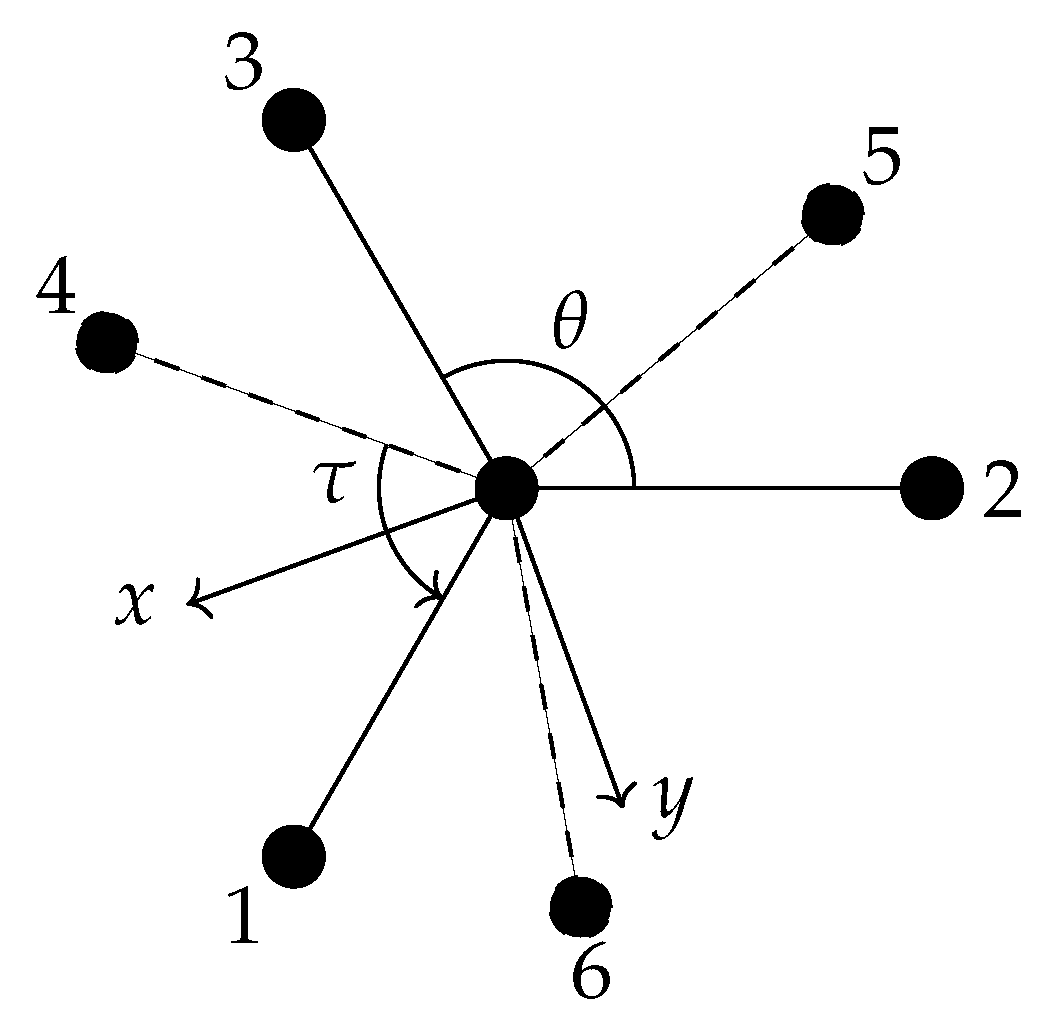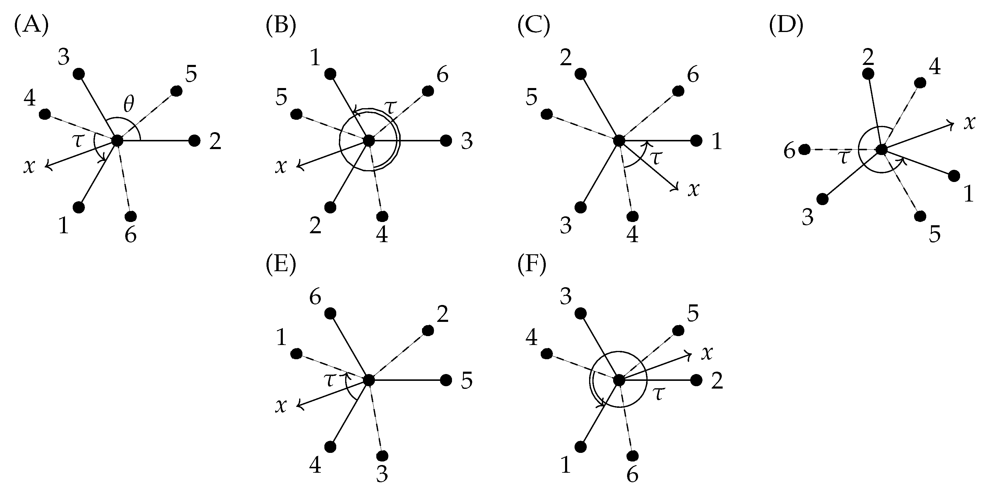For ${\left(123\right)}^3=E$, the changes become $(\tau +4\pi ,\chi +2\pi )=(\tau ,\chi )$ or $(\tau -2\pi ,\chi -\pi )=(\tau +2\pi ,\chi +\pi )$. These are illustrated in Figure 7A,F, respectively.

To deal with the double-valuedness of ($\tau$, $\chi$), we extend the symmetry description in the manner first introduced by Hougen [43], by extending G${}_{36}$ to the extended molecular symmetry group G${}_{36}$(EM) as explained in Section 15.4.4 of [1]. To appreciate the definition of G${}_{36}$(EM), we note that the internal coordinates R, $r_k$ and ${\alpha }_k$ (k = 1, 2, …, 6), ${\gamma }_1$, ${\gamma }_2$, ${\delta }_1$, ${\delta }_2$, $\theta$, and $\varphi$ used for ethane in the present work are all “space-fixed” in the sense of Section 15.4.4 in [1]; the instantaneous values of these coordinates can be unambiguously obtained from the instantaneous coordinate values of the nuclei in a Cartesian, space-fixed axis system [1], e.g., $XYZ$. Appendix C explains in detail how the internal coordinates values are determined from the Cartesian coordinate values.

We present here the ideas of Hougen [43], using the more modern notation of Section 15.4.4 in [1]. The extension of G${}_{36}$ to G${}_{36}$(EM) involves the introduction of a fictitious operation $E^{\prime }$ (taken to be different from the identity E) which, for ethane, we can think of as letting the C_aH₃ do a full torsional revolution relative to the C_bH₃. That is, $E^{\prime }$ has the effect of transforming $\chi$→$\chi +\pi$ and $\tau$→$\tau +2\pi$. After the application of ${\left(E^{\prime }\right)}^2$ the molecule-fixed axis system is back where it started, and so we take ${\left(E^{\prime }\right)}^2$ = E. $E^{\prime }$ does not affect the space-fixed nuclear coordinates; it has the same effect as the identity operation on the complete rotation-torsion-vibration wavefunction of ethane.

We now define four generating operations a, b, c and d that transform $\chi$ and $\tau$ unambiguously and have the same effect on the space-fixed coordinates [R, $r_k$ and ${\alpha }_k$ (k = 1, 2, …, 6), ${\gamma }_1$, ${\gamma }_2$, ${\delta }_1$, ${\delta }_2$, $\theta$, and $\varphi$] as the G${}_{36}$ operations (123), (456), (14)(26)(35)($ab$)${}^{*}$ and (23)(56)${}^{*}$, respectively. Tables A-28 and A-33 of [1] are the character tables of G${}_{36}$ and G${}_{36}$(EM), respectively. Comparison of the two tables shows that the four generating operations $R_2^{(-)}=\left(132\right)\left(456\right)$, $R_2^{(+)}=\left(123\right)\left(456\right)$, $R_4^{(+)}=\left(14\right)\left(26\right)\left(35\right){\left(ab\right)}^{*}$ and $R_4^{(-)}=\left(14\right)\left(25\right)\left(36\right)\left(ab\right)$ chosen for G${}_{36}$ in the present work correspond to $ab$, $a^{5}b$, c, and $dc$, respectively. Following Section 15.4.4 of [1], we define in

Table 4. Transformation of the torsion angle $\tau$ and the rotation angle $\chi$ under the generators of G${}_{36}$(EM).

Transformed $\mathit{\tau }$	Transformed $\mathit{\chi }$	G${}_{36}$(EM) Generator	G${}_{36}$ Generator
$\tau -4\pi /3$	$\chi$	$ab$	(123)(456)
$\tau$	$\chi +2\pi /3$	$a^{5}b$	(132)(456)
$2\pi -\tau$	$\chi +\pi$	c	(14)(26)(35)($ab$)${}^{*}$
$\tau$	$\chi$	$dc$	(14)(25)(36)($ab$)
$\tau +2\pi$	$\chi +\pi$	$E^{\prime }$

the effect on $\chi$ and $\tau$ of the G${}_{36}$(EM) generators. The approach of Bunker and Jensen [1] to simply postulate, by definition, the effect of the G${}_{36}$(EM) generators on $\chi$ and $\tau$ may appear arbitrary. It is not, however. We show in Figure 7 how, for each of the four G${}_{36}$(EM) generators $ab$, $a^{5}b$, c, and $dc$, the effect on $\chi$ and $\tau$ can be explained as the effect of the G${}_{36}$ partner of the G${}_{36}$(EM) generator in question (Table 4).

The group generated by the five operations a, b, c, d, and $E^{\prime }$ has 72 elements and, as mentioned above, it is denoted G${}_{36}$(EM), called an extended molecular symmetry (EMS) group, and its character table is given as Table A-33 of [1]. This character table shows that we can think of G${}_{36}$(EM) as a direct product

$$\mathit{G}{}_{36}\left(\mathrm{EM}\right)=\mathit{G}{}_{36}\times \{E,E^{\prime }\},$$

(29)

where the group ${\mathcal{G}}_{36}$ is constructed from the generating operations a, b, c and d; it is isomorphic to G${}_{36}$, so that it has the irreducible representations given in Table 2. The two-element group $\{E,E^{\prime }\}$ is cyclic of order 2 and has two irreps $A^{\prime }$ and $A^{″}$, both one-dimensional, with the representation matrices 1 or $-1$, respectively, under $E^{\prime }$. The irreps of G${}_{36}$(EM) are straightforwardly constructed from those of G${}_{36}$. Each irrep $\Gamma$ of G${}_{36}$ in Table 2 gives rise to two irreps of G${}_{36}$(EM), ${\Gamma }_s$ = $(\Gamma ,A^{\prime })$ and ${\Gamma }_d$ = $(\Gamma ,A^{″})$ as given in Table A-33 of [1]. An irrep ${\Gamma }_s$ has identical characters for the operations E and $E^{\prime }$, ${\chi }_s\left[E^{\prime }\right]$ = ${\chi }_s\left[E\right]$, whereas for the irrep ${\Gamma }_d$, ${\chi }_d\left[E^{\prime }\right]$ = $-{\chi }_d\left[E\right]$. As long as we pretend that $E^{\prime }$≠E, we must also pretend that the coordinate values $(\tau ,\chi )$ and $E^{\prime }(\tau ,\chi )$ = $(\tau +2\pi ,\chi +\pi )$ describe different physical situations. As a consequence, we must allow $\tau$ to be periodic with a period of $4\pi$ as already mentioned in connection with Equation (21). The torsional potential energy function $V^{1\mathrm{D}}\left(\tau \right)$ is periodic with period $2\pi$, $V^{1\mathrm{D}}\left(\tau \right)$ = $V^{1\mathrm{D}}(\tau +2\pi )$ for $\tau$∈$[0,2\pi ]$, and this symmetry causes the torsional wavefunctions $|n\rangle$ from Equation (21) to be either symmetric (of ${\Gamma }_s$ symmetry) or antisymmetric (of ${\Gamma }_d$ symmetry) under $E^{\prime }$.

We know that, in reality, $E^{\prime }$ = E, and so only functions and coordinates with ${\Gamma }_s$ symmetries occur in nature. Since we can form, for example, basis functions of an allowed ${\Gamma }_s$ symmetry as products of an even number of factors, each with a forbidden symmetry ${\Gamma }_d^{\prime }$, say, we need to consider also the ${\Gamma }_d$ symmetries initially for the torsional and rotational basis functions. The final wavefunctions resulting from our theoretical calculations should be subjected to a “reality check”: They must necessarily have a ${\Gamma }_s$ symmetry in G${}_{36}$(EM). In particular, torsional basis functions of d symmetry must be combined with rotational basis functions of d symmetry to produce a torsion-rotation basis function of an allowed s symmetry.

6.4. Rigid-Symmetric-Rotor Function Representations

As mentioned above, we use the rigid-symmetric-rotor eigenfunctions $|J,k,m\rangle$ [1] as primitive rotational basis functions. For $K\ne 0$ (where $K=\left|k\right|$), the corresponding symmetrised functions are defined as

$$|JKm\eta \rangle =\frac{i^{\eta }{(-1)}^{\sigma }}{\sqrt{2}}(|J,k,m\rangle +{(-1)}^{J+K+\eta }|J,-k,m\rangle )$$

(30)

where

$$\left\{\begin{array}{cc}\sigma =K\mathrm{mod}3\hfill & \eta =1\hfill \\ \sigma =0\hfill & \eta =0,\hfill \end{array}\right.$$

(31)

while for $K=0$ it is $|J00\eta \rangle =i^{\eta }|J,0,0\rangle$ where $\eta =J\mathrm{mod}2$. Using the rigid rotor transformation properties given in Equations (12-46) and (12-47) of [1], along with Tables 12-1 and 15-6 of [1], we can determine the irreps of the rigid rotor basis functions; the results are summarised in

Table 5. The irreps of the rigid rotor wavefunctions. For $K>0$, the two functions with $\eta$ = 0, 1 generate a two-dimensional irrep or the direct sum of two one-dimensional irreps. For a given K value, we list first the $\eta =0$ function and then the $\eta =1$ one. n is a positive integer.

K	$\mathbf{\Gamma }$
0 (J even)	$A_{1s}$
0 (J odd)	$A_{2s}$
$K=3n$ (K even)	$A_{1s}\oplus A_{2s}$
$K=3n$ (K odd)	$A_{4d}\oplus A_{3d}$
$K=3n+1$ (K even)	$E_{1s}$
$K=3n+1$ (K odd)	$E_{2d}$
$K=3n+2$ (K even)	$E_{1s}$
$K=3n+2$ (K odd)	$E_{2d}$

.

6.5. Symmetrisation of the Basis Set

Once a set of basis functions has been constructed for one of the subsets mentioned above as eigenfunctions of a 1D Schrödinger equation, the degenerate eigenfunctions (which in general transform reducibly) are symmetrised by a sampling and projection procedure described in Sections 4 and 5 of [39]. Briefly, a set of geometries is sampled (typically around 50) and each MS operation is applied to the eigenfunctions to obtain an overdetermined set of linear equations which are solved for the transformation matrix effecting the operation on the degenerate eigenfunctions. Using the traces of these matrices and the irrep matrices, one can obtain the irreducible coefficients of the reducible matrix as well as projection operators onto the irreps. These operators are then applied to the eigenfunctions to generate the symmetrised basis functions.

One then produces the basis functions for the complete TROVE calculation as products of the symmetrised 1D basis functions, one 1D basis function from each of the sets defined above. In general, these total basis functions do not transform irreducibly, and so a further application of the symmetrisation procedure is required, although the sampling step can be omitted as the transformation properties of the “factor” functions are already known.

7. Potential Energy Function of Ethane in a Symmetry Adapted Representation

To represent the PES analytically, an on-the-fly symmetrisation procedure has been implemented (see, e.g., [22]). We first introduce the stretching coordinates

$${\xi }_1=1-exp\left(-a(R-R_{\mathrm{e}})\right)$$

(32)

$${\xi }_j=1-exp\left(-b(r_i-r_{\mathrm{e}})\right);j=2,3,4,5,6,7,i=j-1,$$

(33)

(a is used for the C–C internal coordinate R, and b is used for the six C–H internal coordinates $r_1,r_2$, $r_3$, $r_4$, $r_5$ and $r_6$) the bending angular coordinates

$${\xi }_k=({\alpha }_i-{\alpha }_{\mathrm{e}});k=8,9,10,11,12,13,i=k-7,$$

(34)

the dihedral coordinates from Equation (17)

$$\left({\xi }_{14},{\xi }_{15},{\xi }_{16},{\xi }_{17}\right)=\left({\gamma }_1,{\gamma }_2,{\delta }_1,{\delta }_2\right)$$

(35)

and, finally, the torsional term

$${\xi }_{18}=1+cos3\tau$$

(36)

where $\tau$ is defined in Equation (20). The quantities $R_{\mathrm{e}}$, $r_{\mathrm{e}}$ and ${\alpha }_{\mathrm{e}}$ are the equilibrium structural parameter values of C${}_2$H${}_6$.

Taking an initial potential term of the form

$$V_{\mathit{k}}^{\mathrm{initial}}=\prod _{i=1}^{18}{\xi }_i^{k_i}$$

(37)

with maximum expansion order ${\sum }_i{k}_i=6$, each symmetry operation $T_X$ of G${}_{36}$ (see Table 3) is independently applied to $V_{\mathit{k}}^{\mathrm{initial}}$, i.e.,

$$V_{\mathit{k}}^{T_X}=T_X{V}_{\mathit{k}}^{\mathrm{initial}}\left(\mathbf{\xi }\right)=T_X\left(\prod _{i=1}^{18}{\xi }_i^{k_i}\right)$$

(38)

where $T_X$ is one of the 36 operators of G${}_{36}$, to create 36 new terms. Here, $\mathit{k}$ denotes the 18-dimensional hyper-index $k_1,k_2,\dots ,k_{18}$ and $\left(\mathbf{\xi }\right)$ denotes $\{{\xi }_1,{\xi }_2,\dots ,{\xi }_{18}\}$. The results are summed up to produce a final term

$$V_{\mathit{k}}^{\mathrm{final}}=\sum _{T_X}{V}_{\mathit{k}}^{T_X},$$

(39)

which is itself subjected to the 36 G${}_{36}$ symmetry operations $T_X$ to check its invariance. The total potential function is then given by the expression

$$V_{\mathrm{total}}\left(\mathbf{\xi }\right)=\sum _{\mathit{k}}{f}_{\mathit{k}}{V}_{\mathit{k}}^{\mathrm{final}}\left(\mathbf{\xi }\right)$$

(40)

where $f_{\mathit{k}}$ are the corresponding expansion coefficients determined through a least-squares fitting to the ab initio data generated at the CCSD(T)-F12b/aug-cc-pVTZ level of theory. The details of the PES will be given elsewhere. The symmetry operations are represented as matrices and are generated from the four chosen generators as described above (see also Appendix B).

8. Numerical Example

In this section, we apply the symmetrisation procedure on a small test basis set for the ethane molecule. We demonstrate how the method works for Subsets 2 (six C−H${}_i$ stretching modes), 4 (four dihedral-angle modes ${\gamma }_1$, ${\gamma }_2$, ${\delta }_1$, ${\delta }_2$), and 5 (the torsional mode $\tau$). In Subset 1 (C−C stretch), the symmetrised wavefunctions are of $A_{1s}$ symmetry only as each G${}_{36}$ operation leaves the bond length R invariant; in Subset 3 (six C−C−H${}_i$ bending modes), each G${}_{36}$ element has the same effect on the coordinates as in Subset 2, and so the irreps obtained for Subset 3 are identical to those obtained for Subset 2.

In TROVE calculations, the size of the primitive basis set is determined by the maximum polyad number $P_{\max }$, which occurs in the inequality

$$P=a_1{n}_1+a_2{n}_2+a_3{n}_3+\dots \le P_{\max }$$

(41)

where $n_i$ is the excitation number for the primitive basis function of coordinate i and $a_i$ is its polyad coefficient. In our example all $a_i$ = 1.

8.1. Subset 2 Symmetrisation

For the six-member Subset 2, we set the maximum polyad number to be 1, so the space is seven-dimensional. We consider here the seven unsymmetrised eigenfunctions at lowest energy, the latter four being degenerate. As the first three of these eigenfunctions eigenfunctions are non-degenerate, they are already symmetrised and no further work is required. The first one-dimensional energy solution (at 0.0 cm⁻¹)) is essentially the primitive ground-state wavefunction with small contributions from the other primitives:

$${\Psi }_1=0.9999374|000000\rangle +\dots$$

(42)

where … signifies small (of the order ${10}^{-14}$) contributions from other primitive functions (omitted in the following). For simplicity we give only 5–7 significant digits here, while the actual calculations are done in quadruple precision. The eigenfunction in Equation (42) has $A_{1s}$ symmetry.

The second one-dimensional solution (at $2929.16 {\mathrm{c}\mathrm{m}}^{-1}$) is

$${\Psi }_2=\frac{1}{\sqrt{6}}(-|000001\rangle -|000010\rangle -|000100\rangle +|001000\rangle +|010000\rangle +|100000\rangle )$$

(43)

and has $A_{4s}$ symmetry.

The final one-dimensional solution (at $2940.44 {\mathrm{c}\mathrm{m}}^{-1}$) is

$${\Psi }_3=\frac{1}{\sqrt{6}}\left(\right|000001\rangle +|000010\rangle +|000100\rangle +|001000\rangle +|010000\rangle +|100000\rangle )$$

(44)

which is totally symmetric and so of $A_{1s}$ symmetry.

The four unsymmetrised, degenerate solutions (at $3007.21 {\mathrm{c}\mathrm{m}}^{-1}$) are

$$\begin{array}{cc}\hfill {\Psi }_4=& +0.565540|000001\rangle -0.209498|000010\rangle -0.356041|000100\rangle -0.482230|001000\rangle \hfill \\ & -4.233691|010000\rangle +0.524567|100000\rangle \hfill \\ \hfill {\Psi }_5=& -0.536788|000010\rangle +0.446199|000100\rangle +0.330258|001000\rangle -0.578016|010000\rangle \hfill \\ & +0.247758|100000\rangle \hfill \\ \hfill {\Psi }_6=& +0.581276|000001\rangle -0.308888|000010\rangle -0.272388|000100\rangle +0.398602|001000\rangle \hfill \\ & +0.157199|010000\rangle -0.555801|100000\rangle \hfill \\ \hfill {\Psi }_7=& -0.489104|000010\rangle +0.516345|000100\rangle -0.407635|001000\rangle +0.553226|010000\rangle \hfill \\ & -0.145592|100000\rangle \hfill \end{array}$$

(45)

which turn out to be of $G_s$ symmetry, and thus also already symmetrised. However, in this case there is ambiguity in the group matrices describing the transformation properties of the degenerate wavefunctions. We therefore find and apply a unitary transformation on the wavefunctions to produce functions with transformation properties described by our “standard” G representation matrices collected in Appendix B.2. To this end, we follow the sampling procedure from Ref. [39], derive the transformation properties of the above wavefunctions and convert them to have our “standard” transformation properties. For this work, we modified the sampling procedure in TROVE by applying it to the five group generators only (out of 72). This simple modification led to a significant speedup of the sampling part of the code and is now the standard part of TROVE. The reduced symmetrised wavefunctions become

$$\begin{array}{cc}\hfill {\Psi }_4& =\frac{1}{2\sqrt{3}}(-|000001\rangle -|000010\rangle +2|000100\rangle -|001000\rangle -|010000\rangle +2|100000\rangle )\hfill \\ \hfill {\Psi }_5& =\frac{1}{2}(-|000001\rangle +|000010\rangle -|001000\rangle +|010000\rangle )\hfill \\ \hfill {\Psi }_6& =\frac{1}{2\sqrt{3}}(-|000001\rangle -|000010\rangle +2|000100\rangle +|001000\rangle +|010000\rangle -2|100000\rangle )\hfill \\ \hfill {\Psi }_7& =\frac{1}{2}(-|000001\rangle +|000010\rangle +|001000\rangle -|010000\rangle )\hfill \end{array}$$

(46)

which are recognised as the linear combinations (defined by the matrix $\mathbf{V}$) of bond lengths $r_k$ that transform as the $G_s$ irrep (Equation (9)).

8.2. Subset 4 Symmetrisation

For Subset 4, we use a maximum polyad number of 1 and thus we have 5 eigenfunctions, one non-degenerate and four degenerate ones. |0000〉 is the first eigenfunction (at $0.0 {\mathrm{c}\mathrm{m}}^{-1}$); it has $A_{1s}$ symmetry. The other four unsymmetrised eigenfunctions (at $1469.30 {\mathrm{c}\mathrm{m}}^{-1}$) are

$$\begin{array}{cc}\hfill {\Psi }_2& =\frac{1}{\sqrt{2}}\left(\right|0001\rangle -|0100\rangle )\hfill \\ \hfill {\Psi }_3& =-\frac{1}{\sqrt{2}}\left(\right|0001\rangle +|0100\rangle )\hfill \\ \hfill {\Psi }_4& =-\frac{1}{\sqrt{2}}\left(\right|0010\rangle +|1000\rangle )\hfill \\ \hfill {\Psi }_5& =\frac{1}{\sqrt{2}}(-|0010\rangle +|1000\rangle )\hfill \end{array}$$

(47)

which again turns out to be of $G_s$ symmetry. Here, and in the following, $\frac{1}{\sqrt{2}}$ stands for the numerical value $0.707106781186545$ ($\pm {10}^{-15}$). The desired symmetrised functions are

$$\begin{array}{cc}\hfill {\Psi }_2& =\frac{1}{\sqrt{2}}\left(\right|0010\rangle +|1000\rangle )\hfill \\ \hfill {\Psi }_3& =\frac{1}{\sqrt{2}}\left(\right|0001\rangle +|0100\rangle )\hfill \\ \hfill {\Psi }_4& =\frac{1}{\sqrt{2}}\left(\right|0010\rangle -|1000\rangle )\hfill \\ \hfill {\Psi }_5& =\frac{1}{\sqrt{2}}\left(\right|0001\rangle -|0100\rangle ).\hfill \end{array}$$

(48)

8.3. Subset 5 Symmetrisation

For the one-dimensional Subset 5, we use a maximum polyad number of 29 and show, for illustrative purposes, the symmetrisation of the first three eigenfunctions. The lowest energy solution (at $0.0 {\mathrm{c}\mathrm{m}}^{-1}$ with $A_{1s}$ symmetry) is:

$${\Psi }_1=0.999958|0\rangle +\dots .$$

(49)

The second and third eigenfunctions (at $0.0029 {\mathrm{c}\mathrm{m}}^{-1}$) are degenerate, and the unsymmetrised wavefunctions are

$$\begin{array}{cc}\hfill {\Psi }_2=& +0.0272058|1\rangle +0.999588|2\rangle +\dots \hfill \\ \hfill {\Psi }_3=& -0.999588|1\rangle +0.0272058|2\rangle +\dots .\hfill \end{array}$$

(50)

These turn out to be of $E_{3d}$ symmetry, which we then converted to

$$\begin{array}{cc}\hfill {\Psi }_2=& -0.75926|1\rangle -0.65072|2\rangle +\dots \hfill \\ \hfill {\Psi }_3=& -0.65072|1\rangle +0.75926|2\rangle +\dots \hfill \end{array}$$

(51)

to obey our “standard” transformation properties imposed by the matrices in Appendix B.

8.4. Torsional Basis Function Symmetries

Figure 8 shows the torsional potential energy as a function of $\tau$. In order for the torsional basis functions to transform according to the irreps of the extended MS group G${}_{36}$(EM), we obtain them as solutions of the 1D torsional Schrödinger equation in Equation (21). In solving this Schrödinger equation in a Fourier-series basis (see the discussion of Equation (21)), we let $\tau$ vary from 0 to $4\pi$ so that the potential energy curve in Figure 8 has six minima. In the figure, we indicate the lowest allowed torsional energies. Some of these energies are degenerate, i.e., associated with more than one eigenfunction of a given irreducible representation. In the limit of an infinite barrier height, we expect the energies to be six-fold degenerate. With the actual, finite height of the barrier, the energies form near-degenerate clusters with a total multiplicity of 6 as shown in Figure 9. However, since our description of the torsional angle $\tau$∈$[0,4\pi ]$ is unphysical, only three of the states in the cluster (of s symmetry) exist in nature if they are combined with rigid-rotor basis functions of s symmetry. The other three states (of d symmetry) must be combined with rigid-rotor basis functions of d symmetry in order that the total rotation-torsion state can exist in nature. For J = 0, only the s-type torsional states will exist since only s-type rigid-rotor basis functions are available.

Figure 10 shows the ground state torsional wavefunction which, as always, is totally symmetric (of $A_{1s}$ symmetry) in G${}_{36}$(EM). The effect of the G${}_{36}$(EM) generators on $\tau$ is shown in Table 4. In Figure 11 (left display) we show the doubly-degenerate wavefunctions of the first excited state. They span the $E_{3d}$ irrep but must be transformed to obtain the transformation properties imposed by the $E_{3d}$ matrices described in Appendix B.1. The transformed functions, with the desired transformation properties are shown in Figure 11 (right display).

The symmetry adapted ro-vibrational basis set functions are constructed as direct products of the symmetrised component functions from the different subspaces as ${\Psi }_{{\lambda }_0}^{\left(0\right),{\Gamma }_0}\otimes {\Psi }_{{\lambda }_1}^{\left(1\right),{\Gamma }_1}\otimes {\Psi }_{{\lambda }_2}^{\left(2\right),{\Gamma }_2}\cdots \otimes {\Psi }_{{\lambda }_L}^{\left(L\right),{\Gamma }_L}$, where L is the number of vibrational subspaces. The symmetry of a product basis function is the direct product of the irreducible representations of the component functions. This symmetry must be further reduced, but this is rather straightforward when each component function generates one of the irreps of the group and has defined, “standard” transformation properties. In this case, we use the same projection operator symmetrisation technique described above without further sampling of the symmetry properties of the corresponding components. The d-symmetry components are unphysical and must be disregarded. Some s symmetry ro-vibrational basis functions will necessarily contain products of the d components, underpinning the importance of the G${}_{36}$(EM) extended symmetry group. The nuclear spin statistical weights of the ro-vibrational states can be deduced using the procedure from [1]. We obtain nuclear spin statistical weights of 6, 10, 6, 10, 4, 4, 2, 6, and 12 for the G${}_{36}$(EM) symmetries $A_{1s},A_{2s},A_{3s},A_{4s},E_{1s},E_{2s},E_{3s},E_{4s}$, and $G_s$, respectively.

9. Conclusions

We have presented a detailed description of the G${}_{36}$ and G${}_{36}$(EM) molecular symmetry groups. A full set of irreducible representation matrices have been derived and tested for constructing symmetry-adapted potential energy functions and basis functions of ethane C${}_2$H${}_6$. Both the construction of the transformation matrices and the symmetry adaption can be implemented as numerical procedures as part of computational approaches to the solution of the ro-vibrational Schrödinger equation. A self-consistent choice of the vibrational, torsional and rotational coordinates for ethane, satisfying the G${}_{36}$(EM) symmetry requirements, have been introduced and analysed in full detail. The irreducible representation matrices as well as the coordinate choice made for ethane in the present work have been implemented as part of the program system TROVE, and we have discussed a few examples of symmetrised wavefunctions. These results of the present work will be important in our planned line-list calculations for ethane.

The results of the present work are, of course, not only applicable to ethane H${}_3$CCH${}_3$, but also to other molecules with MS groups G${}_{36}$ and G${}_{36}$(EM). A prominent molecule of this kind is dimethylacetylene H${}_3$CCCCH${}_3$. In addition, subgroups of the matrix groups constructed can be applied to molecules whose MS groups are subgroups of G${}_{36}$ and G${}_{36}$(EM), such as D${}_3$CCH${}_3$. The general ideas used for generating the matrix groups can be applied to other MS groups. In particular, generation of matrix groups in a manner similar to that of the present work will be required for MS groups with irreps of dimension 4 and higher.

References

1. Bunker, P.R.; Jensen, P. Molecular Symmetry and Spectroscopy, 2nd ed.; NRC Research Press: Ottawa, ON, Canada, 1998. [Google Scholar]
2. Chubb, K.L.; Jensen, P.; Yurchenko, S.N. Symmetry Adaptation of the Rotation-Vibration Theory for Linear Molecules. Symmetry 2018, 10, 137. [Google Scholar] [CrossRef]
3. Yurchenko, S.N.; Thiel, W.; Jensen, P. Theoretical ROVibrational Energies (TROVE): A robust numerical approach to the calculation of rovibrational energies for polyatomic molecules. J. Mol. Spectrosc. 2007, 245, 126–140. [Google Scholar] [CrossRef]
4. Smeyers, Y.G.; Bellido, M.N. Internal dynamics of nonrigid molecules. I. Application to acetone. Intern. J. Quantum Chem. 1981, 19, 553–565. [Google Scholar] [CrossRef]
5. Carvajal, M.; Álvarez-Bajo, O.; Senent, M.L.; Domínguez-Gómez, R.; Villa, M. Raman and infrared spectra of dimethyl ether 13C-isotopologue (CH3O13CH3) from a CCSD (T) potential energy surface. J. Mol. Spectrosc. 2012, 279, 3–11. [Google Scholar] [CrossRef]
6. Lattanzi, F.; Di Lauro, C. On the Physical Reasons for the Extension of Symmetry Groups in Molecular Spectroscopy. Symmetry 2010, 2, 213–229. [Google Scholar] [CrossRef] [Green Version]
7. Lattanzi, F.; Di Lauro, C. Vibrational symmetry classification and torsional tunneling splitting patterns in G6(EM), G12, and G36(EM) molecules. Mol. Phys. 2005, 103, 697–708. [Google Scholar] [CrossRef]
8. Hougen, J.T. Perturbations in the vibration-rotation-torsion energy levels of an ethane molecule exhibiting internal rotation splittings. J. Mol. Spectrosc. 1980, 82, 92–116. [Google Scholar] [CrossRef]
9. Lattanzi, F.; di Lauro, C. Rotation–Torsion Analysis of the High-Resolution ν6 and ν8 Fundamentals of 70Ge2H6. J. Mol. Spectrosc. 1999, 198, 315–328. [Google Scholar] [CrossRef] [PubMed]
10. Lauro, C.D.; Lattanzi, F.; Valentin, A. Rotational analysis of the ν6, ν8, ν3 + ν4 interacting infrared system of C2D6 between 960 cm−1 and 1180 cm−1. Mol. Phys. 1996, 89, 663–676. [Google Scholar] [CrossRef]
11. Lattanzi, F.; Lauro, C.D.; Horneman, V.M. The high-resolution infrared spectrum of Si2H6: Rotation-torsion analysis of the ν5 and ν7 fundamentals, and torsional splittings in the degenerate vibrational states. Mol. Phys. 2004, 102, 757–764. [Google Scholar] [CrossRef]
12. Lattanzi, F.; Lauro, C.D.; Horneman, V.M. Torsional splittings in the v12 = 1 vibrational state of Si2H6: Analysis of the ν6 + ν12 and ν9 + ν12(E) combination bands in the high resolution infrared spectrum. Mol. Phys. 2006, 104, 1795–1817. [Google Scholar] [CrossRef]
13. Yachmenev, A.; Yurchenko, S.N. Automatic differentiation method for numerical construction of the rotational-vibrational Hamiltonian as a power series in the curvilinear internal coordinates using the Eckart frame. J. Chem. Phys. 2015, 143, 014105. [Google Scholar] [CrossRef] [PubMed]
14. Yurchenko, S.N.; Barber, R.J.; Yachmenev, A.; Thiel, W.; Jensen, P.; Tennyson, J. A Variationally Computed T=300 K Line List for NH3. J. Phys. Chem. A 2009, 113, 11845–11855. [Google Scholar] [CrossRef] [PubMed]
15. Yachmenev, A.; Yurchenko, S.N.; Jensen, P.; Thiel, W. A new “spectroscopic” potential energy surface for formaldehyde in its ground electronic state. J. Chem. Phys. 2011, 134, 244307. [Google Scholar] [CrossRef] [PubMed]
16. Sousa-Silva, C.; Hesketh, N.; Yurchenko, S.N.; Hill, C.; Tennyson, J. High temperature partition functions and thermodynamic data for ammonia and phosphine. J. Quant. Spectrosc. Radiat. Transf. 2014, 142, 66–74. [Google Scholar] [CrossRef]
17. Sousa-Silva, C.; Al-Refaie, A.F.; Tennyson, J.; Yurchenko, S.N. ExoMol line lists - VII. The rotation-vibration spectrum of phosphine up to 1500 K. Mon. Not. R. Astron. Soc. 2015, 446, 2337–2347. [Google Scholar] [CrossRef]
18. Underwood, D.S.; Yurchenko, S.N.; Tennyson, J.; Jensen, P. Rotational spectrum of SO3 and theoretical evidence for the formation of sixfold rotational energy-level clusters in its vibrational ground state. J. Chem. Phys. 2014, 140. [Google Scholar] [CrossRef]
19. Al-Refaie, A.F.; Yurchenko, S.N.; Yachmenev, A.; Tennyson, J. ExoMol line lists IX: A variationally computed line-list for hot formaldehyde. Mon. Not. R. Astron. Soc. 2015, 448, 1704–1714. [Google Scholar] [CrossRef]
20. Yurchenko, S.N.; Tennyson, J. ExoMol line lists—IV. The rotation-vibration spectrum of methane up to 1500 K. Mon. Not. R. Astron. Soc. 2014, 440, 1649–1661. [Google Scholar] [CrossRef]
21. Al-Refaie, A.F.; Ovsyannikov, R.I.; Polyansky, O.L.; Yurchenko, S.N.; Tennyson, J. A variationally calculated room temperature line-list for H2O2. J. Mol. Spectrosc. 2015, 318, 84–90. [Google Scholar] [CrossRef]
22. Owens, A.; Yurchenko, S.N.; Yachmenev, A.; Tennyson, J.; Thiel, W. Accurate ab initio vibrational energies of methyl chloride. J. Chem. Phys. 2015, 142. [Google Scholar] [CrossRef] [PubMed]
23. Owens, A.; Yurchenko, S.N.; Yachmenev, A.; Thiel, W. A global potential energy surface and dipole moment surface for silane. J. Chem. Phys. 2015, 143. [Google Scholar] [CrossRef] [PubMed]
24. Adam, A.Y.; Yachmenev, A.; Yurchenko, S.N.; Jensen, P. Ro-vibrational averaging of the isotropic hyperfine coupling constant for the methyl radical. J. Chem. Phys. 2015, 143, 244306. [Google Scholar] [CrossRef] [PubMed] [Green Version]
25. Owens, A.; Yurchenko, S.N.; Thiel, W.; Spirko, V. Accurate prediction of the ammonia probes of a variable proton-to-electron mass ratio. Mon. Not. R. Astron. Soc. 2015, 450, 3191–3200. [Google Scholar] [CrossRef] [Green Version]
26. Al-Refaie, A.F.; Polyansky, O.L.; Ovsyannikov, R.I.; Tennyson, J.; Yurchenko, S.N. ExoMol line lists—XV. A new hot line list for hydrogen peroxide. Mon. Not. R. Astron. Soc. 2016, 461, 1012–1022. [Google Scholar] [CrossRef]
27. Underwood, D.S.; Tennyson, J.; Yurchenko, S.N.; Huang, X.; Schwenke, D.W.; Lee, T.J.; Clausen, S.; Fateev, A. ExoMol molecular line lists—XIV. The rotation-vibration spectrum of hot SO2. Mon. Not. R. Astron. Soc. 2016, 459, 3890–3899. [Google Scholar] [CrossRef]
28. Owens, A.; Yurchenko, S.N.; Yachmenev, A.; Tennyson, J.; Thiel, W. A global ab initio dipole moment surface for methyl chloride. J. Quant. Spectrosc. Radiat. Transf. 2016, 184, 100–110. [Google Scholar] [CrossRef] [Green Version]
29. Owens, A.; Yurchenko, S.N.; Yachmenev, A.; Tennyson, J.; Thiel, W. A highly accurate ab initio potential energy surface for methane. J. Chem. Phys. 2016, 145. [Google Scholar] [CrossRef]
30. Owens, A.; Yachmenev, A.; Thiel, W.; Fateev, A.; Tennyson, J.; Yurchenko, S.N. ExoMol line lists - XXIX. The rotation-vibration spectrum of methyl chloride up to 1200 K. Mon. Not. R. Astron. Soc. 2018, 479, 3002–3010. [Google Scholar] [CrossRef]
31. Mant, B.P.; Yachmenev, A.; Tennyson, J.; Yurchenko, S.N. ExoMol molecular line lists—XXVII. Spectra of C2H4. Mon. Not. R. Astron. Soc. 2018, 478, 3220–3232. [Google Scholar] [CrossRef]
32. Coles, P.A.; Yurchenko, S.N.; Kovacich, R.P.; Hobby, J.; Tennyson, J. A variationally computed room temperature line list for AsH3. Phys. Chem. Chem. Phys. 2019, 21, 3264–3277. [Google Scholar] [CrossRef] [PubMed]
33. Mant, B.P.; Chubb, K.L.; Yachmenev, A.; Tennyson, J.; Yurchenko, S.N. The infrared spectrum of PF3 and analysis of rotational energy clustering effect. Mol. Phys. 2019, 1–14. [Google Scholar] [CrossRef]
34. Tennyson, J.; Yurchenko, S.N. ExoMol: Molecular line lists for exoplanet and other atmospheres. Mon. Not. R. Astron. Soc. 2012, 425, 21–33. [Google Scholar] [CrossRef]
35. Tennyson, J.; Yurchenko, S.N. The ExoMol project: Software for computing large molecular line lists. Intern. J. Quantum Chem. 2017, 117, 92–103. [Google Scholar] [CrossRef]
36. Al-Refaie, A.F.; Yurchenko, S.N.; Tennyson, J. GPU Accelerated INtensities MPI (GAIN-MPI): A new method of computing Einstein-A coefficients. Comput. Phys. Commun. 2017, 214, 216–224. [Google Scholar] [CrossRef]
37. Longuet-Higgins, H. The symmetry groups of non-rigid molecules. Molecular Physics 1963, 6, 445–460. [Google Scholar] [CrossRef]
38. Available online: http://maxima.sourceforge.net/documentation.html (accessed on 20 September 2018).
39. Yurchenko, S.N.; Yachmenev, A.; Ovsyannikov, R.I. Symmetry adapted ro-vibrational basis functions for variational nuclear motion: TROVE approach. J. Chem. Theory Comput. 2017, 13, 4368–4381. [Google Scholar] [CrossRef]
40. Chubb, K.L.; Yachmenev, A.; Tennyson, J.; Yurchenko, S.N. Treating linear molecule HCCH in calculations of rotation-vibration spectra. J. Chem. Phys. 2018, 149, 014101. [Google Scholar] [CrossRef] [Green Version]
41. Noumerov, B.V. A method of extrapolation of perturbations. Mon. Not. R. Astron. Soc. 1924, 84, 592–602. [Google Scholar] [CrossRef]
42. Cooley, J.W. An Improved eigenvalue corrector formula for solving the Schrödinger equation for central fields. Math. Comp. 1961, 15, 363–374. [Google Scholar] [CrossRef]
43. Hougen, J.T. A Group-Theoretical Treatment of Electronic, Vibrational, Torsional, and Rotational Motions in the Dimethylacetylene Molecule. Can. J. Phys. 1964, 42, 1920–1937. [Google Scholar] [CrossRef]
44. Yamada, K.M.; Winnewisser, G.; Jensen, P. Internal rotation tunnelling in HSOH. J. Mol. Struct. 2004, 695–696, 323–337. [Google Scholar] [CrossRef]
45. Yamada, K.M.; Jensen, P.; Ross, S.C.; Baum, O.; Giesen, T.F.; Schlemmer, S. The torsional and asymmetry splittings in HSOH. J. Mol. Struct. 2009, 927, 96–100. [Google Scholar] [CrossRef]
46. Szalay, V.; Viglaska, D.; Rey, M. Internal- and rho-axis systems of molecules with one large amplitude internal motion: The geometry of rho. J. Chem. Phys. 2018, 149, 244118. [Google Scholar] [CrossRef] [PubMed]
Figure 1. The structure of ethane in the staggered configuration.
Symmetry 11 00862 g001
Figure 2. The labelling of the ethane nuclei.
Symmetry 11 00862 g002
Figure 3. Representative members of three of the vibrational coordinate subsets. Here, R is the C−C bond length, r is one of the six C–H k bond lengths r k , and α is one of the six ∠(H k -C-C) bond angles α k .
Symmetry 11 00862 g003
Figure 4. A Newman projection of ethane, with the CH 3 group containing protons 1, 2, and 3, indicated by solid C−H bonds, being closest to the viewer. One of the dihedral angles used in the vibrational subsets is labelled by θ and the torsional angle is labelled by τ and is measured in the counterclockwise direction. The x axis halves the dihedral angle between the H1−C−C and H4−C−C planes.
Symmetry 11 00862 g004
Figure 5. A Newman projection of ethane, with the CH 3 group containing protons 1, 2, and 3, indicated by solid C−H bonds, being closest to the viewer. The x and y components of the coordinate axes attached to each CH3 group is shown, the subscript a signifying that the coordinate axes are for the CaH3 group. To ensure the coordinate system is right handed, the z axis (the same for both groups) points from Cb to Ca. With this construction, the θ and ϕ Euler describing the direction of the z axis are the same for CH3 group are the same while the χ angle describing the rotation about the z axis different and are denoted by χ a and χ b . These increase in the counterclockwise direction due to the right hand rule.
Symmetry 11 00862 g005
Figure 6. Ethane in the eclipsed configuration.
Symmetry 11 00862 g006
Figure 7. Newman projections of ethane showing the effects of the G 36 (EM) generators (and their G 36 partners; see Table 4) on τ and χ ; the change of τ is represented by the curved arrow encircling the C–C axis and the change of χ is illustrated by the change in x-axis orientation. (A) Starting configuration with τ = 4 π / 9 and the x-axis forming the clockwise angle 8 π / 9 with the horizontal. (B) The effect of a b ∼ (123)(465) which causes τ to decrease by 4 π / 3 (equivalent to an increase of 8 π / 3 ) and χ to remain constant. (C) The effect of a 5 b ∼ (132)(456) with τ remaining constant and χ changing by + 2 π / 3 . (D) The effect of c∼ (14)(26)(35) ( a b ) * with τ 2 π τ and χ χ + π . (E) The effect of d c ∼ (14)(25)(36) ( a b ) under which τ and χ are both invariant. (F) The effect of E which has no G 36 partner, E τ = τ + 2 π and E χ = χ + π .
Symmetry 11 00862 g007
Figure 8. The torsional potential energy as a function of the torsion angle τ . The allowed energy values are marked by blue horizontal lines. Each energy may correspond to more than one eigenfunction of a given irreducible representation. Dashed lines indicate states of d-type symmetry.
Symmetry 11 00862 g008
Figure 9. A enlarged detail of Figure 8, showing the lowest energy cluster with the G 36 (EM) symmetry labels indicated.
Symmetry 11 00862 g009
Figure 10. The ground state torsional wavefunction.
Symmetry 11 00862 g010
Figure 11. The degenerate first excited state torsional wavefunctions. (Left) The two wavefunctions which generate the E 3 d irrep, but which do not transform as given by the transformation matrices of Appendix B.1, displayed as a red and a blue curve, respectively. (Right) The corresponding two E 3 d wavefunctions obtained as transforming according to the transformation matrices of Appendix B.1 and displayed as a red and a blue curve, respectively.
Symmetry 11 00862 g011