Personalized Product Evaluation Based on GRA-TOPSIS and Kansei Engineering


1
School of Mechanical Engineering, Guizhou University, Guiyang 550025, China
2
Key Laboratory of Advanced Manfacturing Technology of the Ministry of Education, Guizhou University, Guiyang 550025, China
3
Department of Computer Science and Engineering, University of South Carolina, Columbia, SC 29208, USA
*
Authors to whom correspondence should be addressed.
Symmetry 2019, 11(7), 867; https://0-doi-org.brum.beds.ac.uk/10.3390/sym11070867
Submission received: 27 April 2019
/
Revised: 4 June 2019
/
Accepted: 21 June 2019
/
Published: 3 July 2019
(This article belongs to the Special Issue Multi-Criteria Decision-Making Techniques for Improvement Sustainability Engineering Processes)
Abstract
:With the improvement of human living standards, users’ requirements have changed from function to emotion. Helping users pick out the most suitable product based on their subjective requirements is of great importance for enterprises. This paper proposes a Kansei engineering-based grey relational analysis and techniques for order preference by similarity to ideal solution (KE-GAR-TOPSIS) method to make a subjective user personalized ranking of alternative products. The KE-GRA-TOPSIS method integrates five methods, including Kansei Engineering (KE), analytic hierarchy process (AHP), entropy, game theory, and grey relational analysis-TOPSIS (GRA-TOPSIS). First, an evaluation system is established by KE and AHP. Second, we define a matrix variate—Kansei decision matrix (KDM)—to describe the satisfaction of user requirements. Third, the AHP is used to obtain subjective weight. Next, the entropy method is employed to obtain objective weights by taking the KDM as input. Then the two types of weights are optimized using game theory to obtain the comprehensive weights. Finally, the GRA-TOPSIS method takes the comprehensive weights and the KMD as inputs to rank alternatives. A comparison of the KE-GRA-TOPSIS, KE-TOPSIS, KE-GRA, GRA-TOPSIS, and TOPSIS is conducted to illustrate the unique merits of the KE-GRA-TOPSIS method in Kansei evaluation. Finally, taking the electric drill as an example, we describe the process of the proposed method in detail, which achieves a symmetry between the objectivity of products and subjectivity of users.
1. Introduction
Products are the material basis for the survival and development of enterprises [1,2]. With the increasing market competition, only by launching products that meet users’ requirements can enterprises increase user satisfaction, stimulate their purchase desire, and boost sales [3,4]. In this case, developing an appropriate method to rank products that reflect user satisfaction is critical. As living level improving, users’ requirements changing from function to emotion, which has been studied using Kansei engineering (KE) approach. The “Kansei” is a Japanese word that contains sensibilities, impressions, and emotions of human [5,6]. Different users may prefer different products. Therefore, this paper aims to make a subjective user personalized ranking of products and pick out the most suitable one for users. The product selection issue can be seen as a multi criteria decision-making (MCDM) problem.
MCDM involves a complex external environment and many different attributes. Many methods have been proposed to solve the MCDM problem. The techniques for order preference by similarity to ideal solution (TOPSIS) is one of effective and powerful methods, which was developed by Hwang and Yoon [7]. Its conception is to find a positive ideal solution (PIS) and a negative ideal solution (NIS) as comparison standards for each alternative. By comparing the degree of differentiation between the ideal solutions and alternatives, the disparity of alternatives can be acquired. The most suitable alternative should be nearest to the PIS and farthest from the NIS. Lei et al. [8] applied the TOPSIS method to assess engines. The closeness, which is used to rank alternatives, is obtained by calculating the Euclidean distance between the alternative and the ideal solutions. They selected circulating water temperature difference, engine oil temperature, turbocharger’s boost temperature, intercooler’s decreased temperature, fuel consumption, and maximum torque as criteria for evaluation. The six criteria are positive indicators, which means that the higher the better. Therefore, take maximum values to construct the PIS and minimum values to build the NIS.
In TOPSIS, measuring the separation of each alternative from the PIS and NIS is a critical part. Moreover, there are other distance metrics besides Euclidean distance, such as Manhattan [9], Chebyshev [10], Hamming [11], and Minkowski [12], etc. In MCDM, since it is impossible to build a unique mathematical model to compare the performance of these distance metrics, the selection always depends on the decision-maker’s (DM’s) assessments [13]. Moreover, Euclidean distance is the most popular distance metrics [14].
With the deepening realization about the TOPSIS method, some extended methods have emerged. Sakthivel et al. [15] combined grey relational analysis (GRA) with TOPSIS to propose the GAR-TOPSIS method. Its closeness is a combination of the grey relational degree and the Euclidean distance. They selected brake thermal efficiency, exhaust gas temperature, oxides of nitrogen, smoke, hydrocarbon, carbon monoxide, and carbon dioxide as criteria to evaluate fuel blends. The seven criteria are cost criteria, which means that the lower the better. Therefore, take minimum values to construct the PIS and maximum values to build the NIS. Şengül et al. [16] adopted fuzzy TOPSIS to rank power stations. The fuzzy ideal solutions are used instead of the ideal solutions to calculate the closeness. They selected nine criteria, including both benefit and cost criteria. The fuzzy PIS is constructed with maximum values of benefit criteria (CO2 emission, job criterion, efficiency, installed capacity, and the amount of energy produced) and minimum values of cost criteria (investment cost, operation cost, land use, and payback period). The fuzzy NIS is constructed with benefit criteria’s minima and cost criteria’s maxima.
As mentioned above, in TOPSIS and its extension methods, their criteria are function property values (such as charging efficiency in the power station ranking problem), either the higher the better, or the lower the better. For the human perception of products, people only care about whether the criteria satisfy their requirements, rather than the exact values of the criteria. The more user requirements (which are usually subjective) are satisfied the better, and vice versa. Considering the huge difference between the criteria users used in the perceptual evaluation and the objective criteria measured from the products, TOPSIS and its extension methods cannot be used directly to make a subjective user personalized ranking of products. Since KE is a feasible method of processing criteria for user-based evaluation, it can make the processed criteria suitable for applying TOPSIS and its extension methods to user-specific subjective product evaluation. Moreover, since perception is uncertain and GRA-TOPSIS can measure the uncertainty between things [13,17], this research adapts GRA-TOPSIS and KE to rank product alternatives.
Determining the weight of individual criterion is an essential part of the TOPSIS and its extension methods. Once the weight is determined, all alternatives can be compared based on the aggregate performance of all criteria. The weights of criteria are categorised as subjective, objective, and combinative. The subjective weighting method based on subjective preferences of the DM or expert, including the Delphi method [18], the AHP method [19], the stepwise weight assessment ratio analysis (SWARA) [20], the factor relationship (FARE) [21], the best–worst method (BWM) [22], KEmeny median indicator ranks accordance (KEMIRA) [23], etc. As the number of criteria increases, the MCDM problem can become intricate, and the DM/expert may not be able to assign a precise weight for each criterion. The objective weighting method extracts statistical weights through dispersion analyses of the data, including entropy [24], data envelopment analysis (DEA) [25], and the criteria importance through inter-criteria correlation (CRITIC) method [26]. The combinative weighting method is a compromise between the subjective and objective [27]. It can not only express the preference of the DM/expert, but also consider the intrinsic information of criteria. Concretely, the subjective and objective weights are combined by the combination principle to obtain comprehensive weights. Commonly used combination principles are multiplication, addition, game theory [28], and evidence theory [29,30]. AHP and entropy are the most useful and practical methods. We believe that reasonable weights should take into account both subjective preferences and objective information. Therefore, this paper uses AHP and entropy to obtain two types of weights and integrate them based on game theory.
Table 1 summarizes some methods of MCDM in the literature. Although various extended TOPSIS methods have been successful in ranking alternatives, there are few approaches from the Kansei point of view. Due to the complexity and uncertainty of the perception, product evaluation becomes a very complicated task. Therefore, this paper integrates five methods (KE, AHP, entropy, game theory, and GRA-TOPSIS) to construct a hybrid KE-GRA-TOPSIS method, which ranks alternatives from criteria and users’ requirements. The main contributions of this paper are summarized as follows.
- We define a matrix variate (Kansei decision matrix, KDM) to describe the satisfaction of user requirements. The KDM taking a user’ requirements as the PIS, and the farthest from requirements constitute the NIS. To extend MCDM methods to user-specific subjective product evaluation, we replace the decision matrix with KDM.
- Taking the KDM as input, the entropy method is used to acquire the objective weights. Moreover, adopt AHP to get subjective weights. Then, the game theory is used to optimize the two types of weights to obtain comprehensive weights, which is one of the inputs of KE-GRA-TOPSIS.
- We combine AHP and KE to construct user requirements into a hierarchy (evaluation system). Specifically, we adopt AHP to establish a hierarchical structure, and KE is used to obtain criteria and indexes.
- Taking the electric drill as an example, we compared DM’s choice with the ranking results of KE-GRA-TOPSIS, KE-TOPSIS, KE-GRA, GRA-TOPSIS, and TOPSIS methods. It is shown that KE-GRA-TOPSIS outperforms other methods in terms of accuracy.
The rest of this paper is organized as follows. In Section 2, we present the general framework firstly. Then we describe the KE, AHP, entropy method, game theory, and GRA-TOPSIS method in detail. In Section 3, the feasibility and effectiveness of the proposed method is verified through an example, and the related experimental results are presented. Finally, the conclusions of this study are provided in Section 4.
2. Methods
2.1. Research Framework
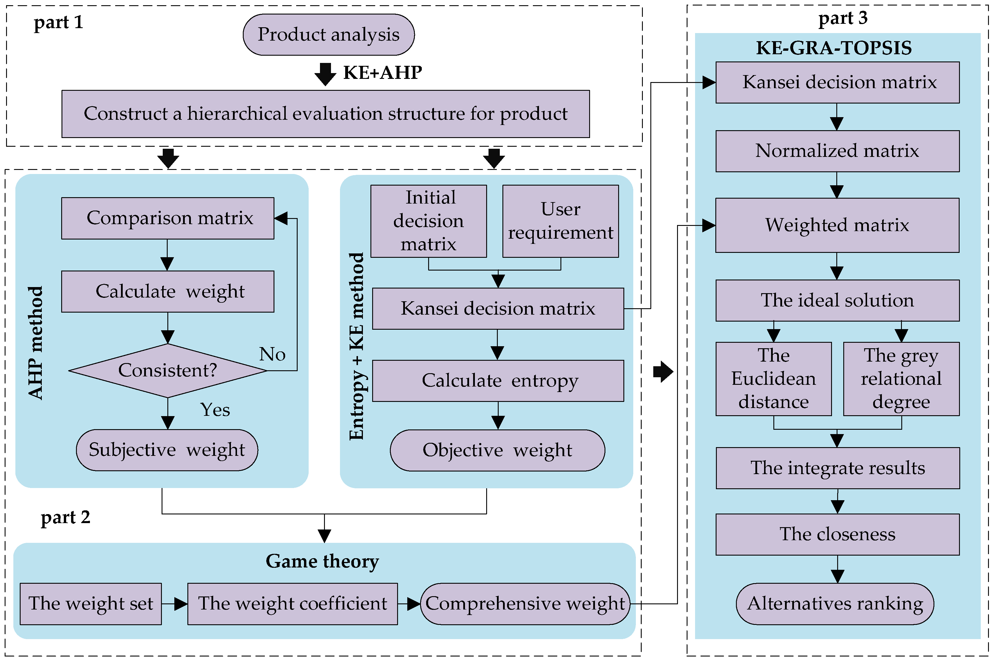
To make a subjective user personalized ranking of alternative products, this research combines KE, AHP, entropy, game theory, and GRA-TOPSIS to form a KE-GRA-TOPSIS method. As shown in Figure 1, the KE-GRA-TOPSIS method contains three parts. In part 1, the KE and AHP methods are used to construct a hierarchical evaluation structure for products. In part 2, the AHP method is used to calculate the subjective weights, which must pass a consistency check. Moreover, the semantic differential (SD) method is used to construct the KDM based on the initial decision matrix and user requirements. Then, the entropy method is used to calculate the objective weights. Finally, game theory is used to obtain the optimal weights based on subjective weights and objective weights. The optimal weights are later used in the GRA-TOPSIS method. In part 3, the weighted matrix is formed based on the KDM and the comprehensive weights in part 2. Next, determine the ideal solutions. Then, calculate the Euclidean distance and grey relational degree between each alternative and the ideal solutions. After that, we can obtain integrated results and closeness. Finally, all the alternatives are ranked in a descending order based on the value of closeness. The alternatives with higher rank can meet user requirements better.
2.2. KE Method
Kansei refers to the feelings that people experience when the outside world stimulates them. The stimulation includes many aspects such as sight, hearing, touch, and smell. Kansei is a comprehensive evaluation of humans, which plays a vital role in product design. Sometimes even users cannot express their requirements with clear words. Research on Kansei is an important means of meeting user needs. KE is a combination of Kansei and engineering, and it is one of the main areas of ergonomics [34]. In ergonomics and psychology, adjectives are often used to describe persons feeling of products. Since there may be correlations, redundancies, and similarities between adjectives, a pair of adjectives with opposite meanings can better reflect human psychology. In KE, such words are called as Kansei words [6].
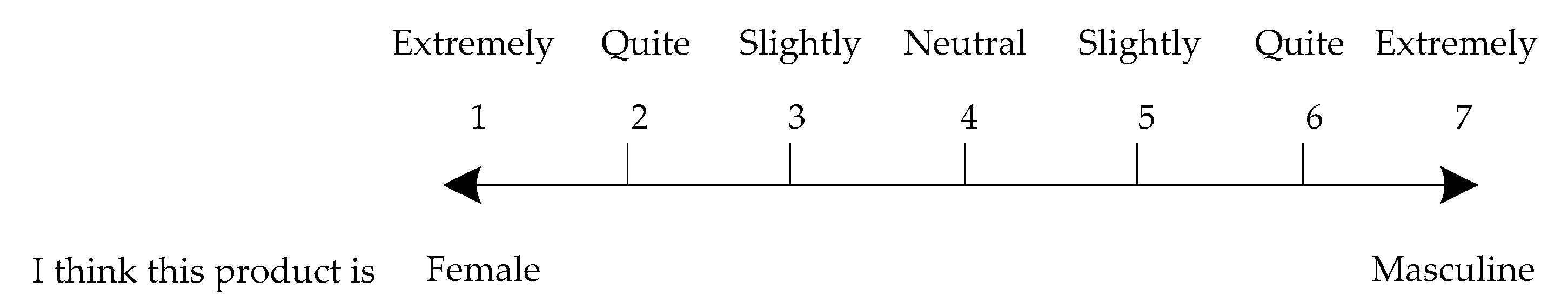
The SD method is widely used to quantify human perception [5,35,36]. The SD scale is the key to the SD method, which consists of bipolar scales and N-point rating scale. Typically, the bipolar scale is a pair of Kansei words, and the grade of N is five, seven, and nine. An example of a seven-point scale is shown in Figure 2.
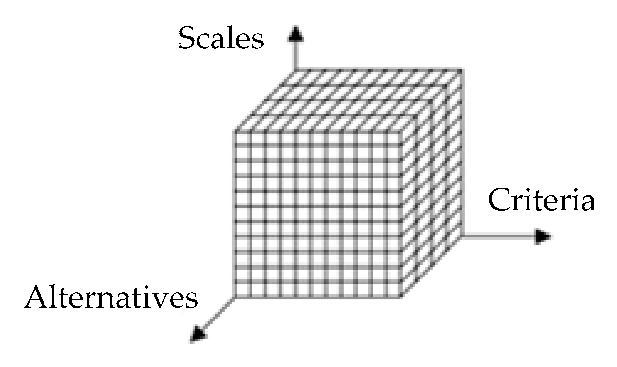
Users evaluate the perception (“Criteria” axis) of the product ("Alternatives" axis) based on the SD scale ("Scales" axis) to obtain a matrix (Figure 3). The matrix represents users’ Kansei evaluation of the product.
Formation of the Kansei evaluation matrix (also called initial matrix) based on m alternatives (A = {Ai, i = 1, 2, …, m}) and n criteria (C = {Cj, j = 1, 2, …, n}). The matrix H is as described in Equation (1). hij is the evaluation value of the jth criterion index of the ith alternative.
As user requirements U= {Uj, j = 1, 2, …, n} of products vary from person to person. Therefore, we define a KDM B to describe the degree of satisfaction. In matrix B, the user requirements constitute the PIS, and the farthest values from requirements constitute the NIS. Matrix B (Equation (2)) is constructed by Equation (3).
where bij is an element of matrix B corresponding to the jth criterion of ith alternative. N is the grade of the SD scale.
2.3. AHP Method
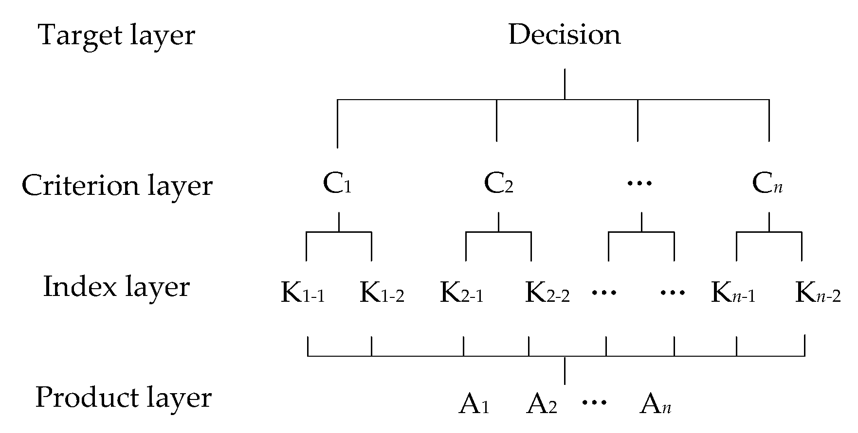
The AHP is a combination of qualitative and quantitative analysis, which was proposed by Saaty [37,38]. The core concept of AHP is decomposing a complex problem into a hierarchic structure, and assess the relative importance of these criteria by pairwise comparison. The hierarchy is constructed in such a way that the goal is at the top, criteria and indexes are in the middle, and alternatives at the bottom, as shown in Figure 4. The criteria link the alternatives to the goal. In this research, we take Kansei words as indexes.
Using the AHP to obtain weights, the pairwise comparison matrix is necessary. It is constructed by comparing the importance of two factors using Saaty scale. The detailed assignment of the Saaty scale is shown in Table 2. For n factors, the total number of comparisons is = n × n(n − 1)/2.
Let O represent an n × n pairwise comparison matrix, which is described in Equation (4). oij is the importance of the ith to the jth factor. For matrix O, the diagonal elements are self-comparison. Thus, oij = 1, where i = j. oij and oji are symmetric about the diagonal of the matrix. Thus, oij = 1/oji, where oij > 0.
The subjective weight matrix W1 = (w1, w2, …, wn) is obtained by Equation (5). Moreover, the objective weight is later used in game theory.
The maximum eigenvalue λmax of O is obtained by Equation (6).
A consistency check is necessary to ensure the rationality of the pairwise comparison matrix. Consistency Ratio (CR) is an indicator of consistency, it is calculated by Equation (7).
where n is the number of criteria. Consistency Index (CI) is estimated as (λmax − n)/(n − 1). Random index (RI) is defined in Table 3. If CR ≤ 0.1, the comparison matrix is reasonable; otherwise, it needs to be modified.
2.4. Entropy Method
The information entropy theory was first introduced to information systems from thermodynamics by Shannon [39]. According to the information entropy theory, the entropy can reflect the degree of diversity within a criterion dataset [26,27]. The greater the degree of diversity, the higher the weight of this criterion, and vice versa.
In this research, the entropy method begins with the Kansei matrix B, which described in Equation (1). To determine objective weights by the entropy method, matrix B needs to be normalized. The normalized matrix P can be represented as Equation (8). pij is the normalized value, which can be calculated by Equation (9).
The entropy of the jth criterion (Ej) can be calculated by Equation (10).
where K = 1/ln(m) is constant.
The degree of divergence (dj) can be calculated by Equation (11).
dj is the inherent contrast intensity of Cj. The more divergent the performance rating pij is, the more critical the criterion Cj is for the problem.
The objective weight (W2 = {wi, j = 1, 2, …, n}) for each criterion Cj (j = 1, 2, …, n) is calculated by Equation (12). Moreover, the objective weight is later used in game theory.
2.5. Game Theory
As mentioned previously, there are certain drawbacks whether objective or subjective weighting methods. The objective weight neglects the DM’s preference and the actual situation. Conversely, the subjective weight neglects the intrinsic information of the criteria. Therefore, the comprehensive weights, combining the subjective and objective weights with a combination principle, is more reasonable.
Game theory is a method originated from modern mathematics, and it is employed to obtain the optimum equilibrium solution among two or more participants [28,30,32]. In game theory, each participant wants to maximize his payoff, which requires them to reach a collective decision that makes every participant obtain the best payoff. The decision involves consensus and compromises. In this research, to make the comprehensive weight have both the subjective preference and objective information, we regard this problem as a “weight” game, the subjective and objective weights are participants, and comprehensive weights are the collective decision.
A basic weight vector set W = {W1, W2, …, WL} is constructed by L kinds of weights. A possible weight set is constructed by arbitrary linear combinations of L vectors. It can be described as Equation (13).
where α = (α1, α2, …, αL) is the weight coefficient and w is a possible weight vector in set W.
According to the game theory, the obtain of the optimum equilibrium weight vector w* can be regarded as optimization of αk. The αk is a linear combination. The optimization is aiming to minimize the deviation between w and wk. It can be expressed as Equation (14).
The optimal first-order derivative condition of Equation (14) is shown in Equation (15), based on the differentiation property of the matrix.
Equation (15) can be converted into a system of linear equations as shown in Equation (16).
α can be calculated by Equation (16) and normalized by Equation (17).
Lastly, the comprehensive weight w* is calculated by Equation (18). The comprehensive weight is later used in the GRA-TOPSIS method.
2.6. GRA-TOPSIS Method
In 1994, Tzeng et al. [40] illustrated similarities of the grey relation model and TOPSIS in the input and process. In a subsequent study [17], they proposed the GRA-TOPSIS method to evaluate alternatives. The idea of the GRA-TOPSIS method is as follows. First, construct a PIS and NIS through the TOPSIS method. Secondly, adopt GRA to calculate the gray correlation degree. Third, calculate the Euclidean distance by TOPSIS. Finally, aggregate the gray correlation degree and the Euclidean distance to obtain the closeness [33]. According to the closeness, the alternatives are ranked. The specific steps are as follows.
Step 1: Constructing the decision matrix.
In this research, we replace the decision matrix with the KDM B, which is described in Equation (2).
Step 2: Calculating the normalized decision matrix.
The normalized decision matrix R is described in Equation (19). rij is the normalized value, which can be calculated by Equation (20).
Step 3: Calculating the weighted decision matrix.
The matrix Z is based on the matrix B and the comprehensive weight w* = (w1, w2, …, wn). It is described in Equation (21). zij is the weighted value, which can be calculated by Equation (22).
Step 4: Determining the ideal solutions.
The ideal solutions include the PIS A+ = (, , …, ) and NIS A− = (, , …, ). They are determined by Equations (23) and (24), respectively.
Step 5: Calculating the separation of each alternative from the PIS and NIS.
We use Euclidean distance to measure the separation of each alternative from the PIS and NIS. The separations are defined in Equations (25) and (26).
where represents the distance between alternative Ai and A+. represents the distance between alternative Ai and A−.
Step 6: Calculating the grey relational coefficients.
The grey relational coefficients can be calculated by Equations (27) and (28), respectively.
where ρ is the distinguishing coefficient, ρ ϵ [0, 1]; ρ = 0.5 is usually applied following the rule of least information [41].
Step 7: Calculating the grey relational degree and integrated results.
The grey relational degrees are calculated by Equations (29) and (30), respectively.
The dimensionless processing is performed on , , and , and the integrate results are obtained by Equations (31) and (32).
where β is the influence coefficient of the distance from alternative to the ideal solution on the closeness. γ is the influence coefficient of the grey relational degree of the alternative and the ideal solution on the closeness. β, γ ϵ [0, 1], β + γ = 1.
Step 8: Calculating the closeness and ranking the alternatives.
The closeness Ci is defined to determine the ranking order of all alternatives. It is calculated by Equation (33).
If the alternative Ai is closer to A+ and farther from A−, Ci is more approximate to 1. Therefore, we can pick out the best-fit one among all alternatives.
3. Empirical Study
To illustrate the possibilities for the application of the proposed method, we conducted a case study of electric drill selection. It has the following steps; (1) use KE and AHP to construct an evaluation structure, (2) adopt AHP to obtain the subjective weights, (3) adopt entropy to obtain the objective weights, (4) employ game theory to get the comprehensive weights, (5) adopt the SD method to build the KDM, and (6) use GRA-TOPSIS to rank alternatives.
3.1. Evaluation System and Alternatives
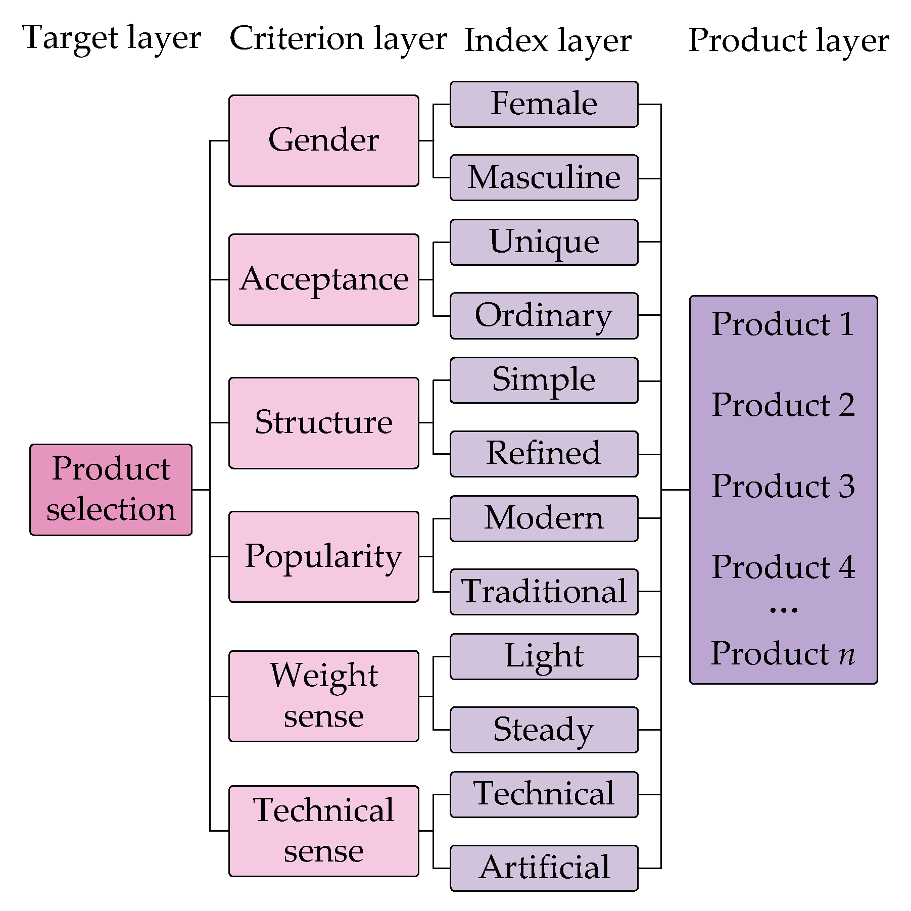
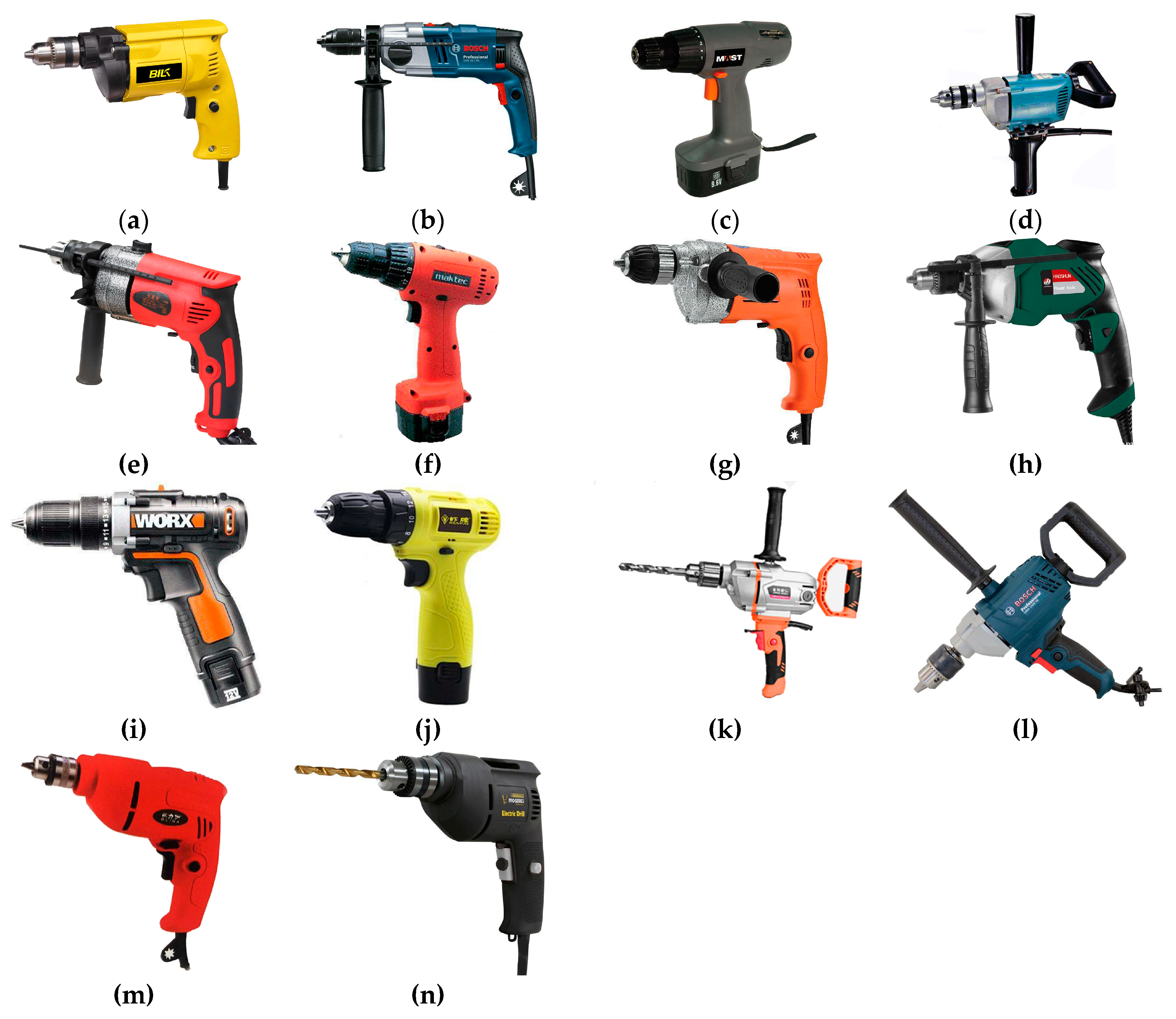
To evaluate the perception of electric drills, we use AHP and KE to establish a hierarchy shown in Figure 5. The target layer has only one element, which is product selection. We have identified six criteria as the dimensions for Kansei evaluation: “Gender”, “Acceptance”, “Structure”, “Popularity”, “Weight sense”, and “Technical sense”. Each criterion includes a pair of Kansei words. “Gender” comprising “Female” and “Masculine”. “Acceptance” comprising “Unique” and “Ordinary”. “Structure” comprising “Simple” and “Refined”. “Popularity” comprising “Modern” and “Traditional”. “Weight sense” comprising “Light” and “Steady”. “Technical sense” comprising “Technical” and “Artificial”. The difference in the color, trigger switch, air vent, chuck, model, name label, etc. of electric drills has led to different evaluation results. We selected 14 electric drills as the alternatives, and they are shown in Figure 6.
3.2. Criteria Weighting
In this research, we take the DM (also called as user) requirements as “extremely masculine”, “slightly ordinary”, “quite simple”, “slightly modern”, “quite light”, and “slightly technical”. We need to match an electric drill closest to the DM requirements in the given 14 alternatives. Based on the 7-point SD scale, the DM requirements can be expressed as U = [7,5,2,3,2,3]. The selection of the electric drill is as follows.
First, the DM is invited to construct a pairwise comparison matrix based on Equation (1). Then, according to Equations (5) and (6), the subjective weights and the maximum eigenvalue are obtained. Finally, we finished the consistency check based on Equation (7). The results are shown in Table 4.
We constructed the questionnaire (Figure 7) and invited 30 people (10 designers and 20 consumers) to evaluate of 14 electric drills in six dimensions, and the average of the results (Table 5) constitute an initial decision matrix H.
According to Equations (3) and (9), the KDM B and the normalized matrix P are obtained as
Then the entropy E and objective weight w of each criterion are calculated by using Equations (10)–(12). The specific calculation results are shown in Table 6.
We have acquired subjective and objective weights, and then we will optimize them based on game theory. Using Equations (16) and (17), we can get the weight coefficient α = (0.4331,0.5669). According to Equation (18), the comprehensive weight is obtained, i.e., w* = (0.2541, 0.1583, 0.213, 0.1316, 0.0844, 0.1584).
3.3. Alternative Ranking
According to Equations (20) and (22), the normalized matrix R and the weighted decision matrix Z are obtained as
According to Equations (23) and (24), the positive ideal solution A+ and the negative ideal solution A− are determined, that is, A+ = [0.0907 0.0543 0.0804 0.0447 0.0321 0.0487], A− = [0.0209 0.0315 0.0291 0.024 0.016 0.0283]. Then, the distances and the grey relational coefficients are obtained by Equations (25)–(30), which is shown in Table 7.
To illustrate the unique merits of KE-GRA-TOPSIS in Kansei evaluation, a comparison of KE-GRA-TOPSIS, KE-TOPSIS, and KE-GRA is conducted in this study. In Equations (31) and (32), β and γ denote the proportion of TOPSIS and GRA in GRA-TOPSIS, respectively. When β = 1, γ = 0 indicates only the TOPSIS method is used; when β = 0, γ = 1 indicates only the GRA method is used. According to Equations (31) and (32), the comparison integrated results are obtained in Table 8.
According to Equation (33), the closeness and ranking of KE-GRA-TOPSIS, KE-TOPSIS, and KE-GRA are obtained. The comparison results are shown in Table 9.
As shown in Table 8, both KE-GRA-TOPSIS and KE-TOPSIS recommend A6 as the best-fit product for user requirements (“extremely masculine”, “slightly ordinary”, “quite simple”, “slightly modern”, “quite light”, and “slightly technical”). This predicted result is the same as the DM’s choice. KE-GRA recommends A3 as the best-fit product. In this experiment, the DM is the user, so we take the DM’s ranking results as the comparison standard for the other three methods. The symbol ‘’ means “better than”, and the DM’s ranking can be expressed as . The ranking of KE-GRA-TOPSIS is . Compared to the standard, the order of A4, A13, and A14 are confused. Three out of fourteen are wrong. The ranking of KE-TOPSIS is . The order of A1 and A10 is reversed, as are A3 and A4, A5 and A9. Six out of fourteen are wrong. The ranking of KE-GRA is . Only A12 is correct. These results imply that the KE-GRA-TOPSIS method has the highest accuracy, followed by the KE-TOPSIS method, and the KE-GAR method has the lowest accuracy. This experiment verifies the feasibility of the KE-GRA-TOPSIS method.
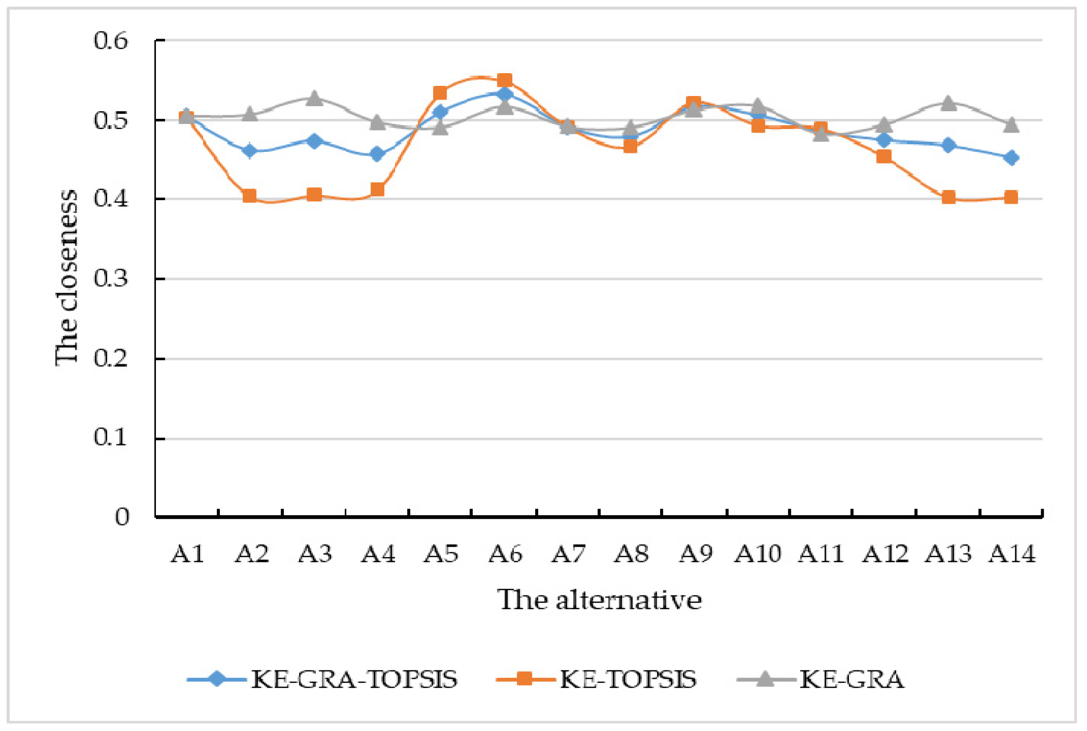
Figure 8 is drawn according to the closeness results in Table 9. As shown in Figure 8, there is a big gap in the closeness of alternatives in KE-TOPSIS, because it only considers the distance of alternatives, amplifying the evaluation results. The gap between alternatives in KE-GRA is relatively small, as this method focuses on the connection between criteria but ignores the distance between alternatives. The KE-GRA-TOPSIS takes into account both the connections between the criteria and the distance between alternatives, so its closeness is more in line with the actual situation.
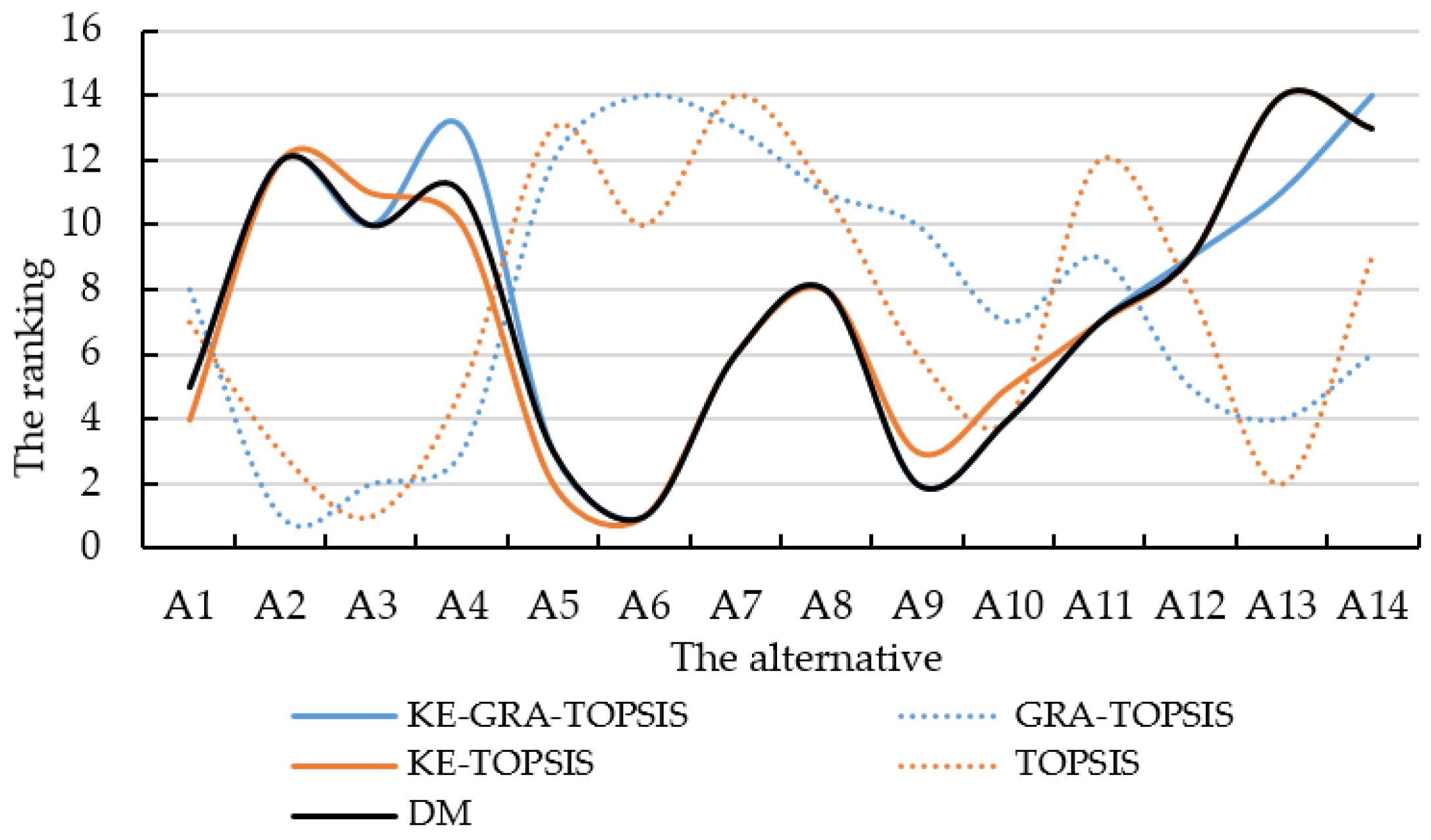
We also compared the choice of DM with the results of KE-GRA-TOPSIS, GAR-TOPSIS, KE-TOPSIS, and TOPSIS. The comparison results are shown in Table 10. Since the accuracy of KE-GRA is too low to be effective, we canceled it in the comparative method. As shown in Table 10, KE-GRA-TOPSIS has the highest accuracy rate of 78.6%, followed by 57.2% of KE-TOPSIS. Moreover, the accuracies of GAR-TOPSIS and TOPSIS are 7.2% and 0, respectively. Figure 9 is drawn according to Table 10. In Figure 9, we can easily find that the results of KE-GAR-TOPSIS and KE-TOPSIS are similar, while GRA-TOPSIS and TOPSIS are similar. Furthermore, the results of KE-GAR-TOPSIS and KE-TOPSIS are roughly consistent with the DM’s choice. This experiment verifies the TOPSIS and its extension methods cannot be used directly to make a subjective user personalized ranking of products.
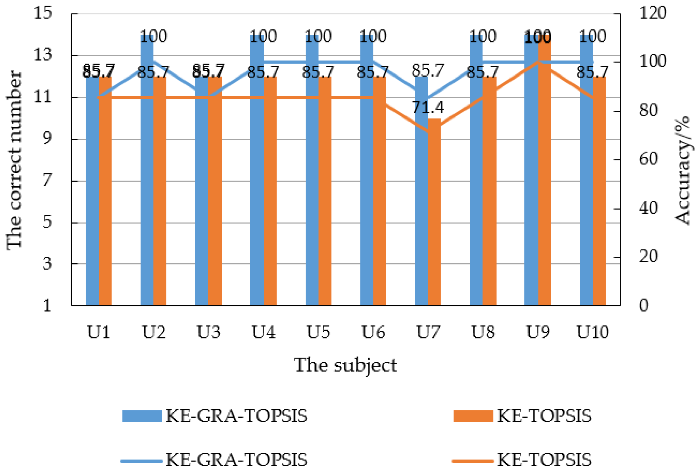
To illustrate the effectiveness of the proposed method, we invited another 10 participants to repeat the experiment. Table 11 shows the requirements and ranking results given by the participants. It is worth noting that the subjective weights in AHP are adjustable. In this experiment, all the participants agreed to use the weights in Table 4. The results are shown in Figure 10.
In Figure 10, the bar chart shows the correct ranking number and the line chart is the accuracy. In KE-GRA-TOPSIS, the accuracy of U1–U10 is 85.7%, 100%, 85.7%, 100%, 100%, 100%, 85.7%, 100%, 100%, and 100%. Its average is calculated as 95.7%. In TOPSIS, the accuracy of U1–U10 is 85.7%, 85.7%, 85.7%, 85.7%, 85.7%, 85.7%, 71.4%, 85.7%, 100%, and 85.7%. Its average is calculated as 85.7%. Their accuracy implies that the KE-GRA-TOPSIS and KE-TOPSIS perform well, and KE-GRA-TOPSIS is more accurate than KE-TOPSIS.
The above results show that the Kansei evaluation matrix is feasible, and the KE-GAR-TOPSIS method can accurately rank products based on user requirements. An accurate prediction can lead to an accurate recommendation. Moreover, the accurate recommendation can increase user satisfaction, stimulate the purchase desire, and expand the sales of production enterprise. Furthermore, it can help enterprises to increase market occupancy in the highly competitive marketplace.
4. Conclusions
We propose the KE-GRA-TOPSIS method to evaluate product design alternatives, according to both the criterion and user requirements. Firstly, we use KE and AHP to establish an evaluation system. Second, we use AHP to obtain subjective weights. Third, in order to get objective weights based on the entropy method, we introduced a KDM, which is a combination of the initial decision matrix and user requirements. In the process of constructing the KDM, we adopt an SD method and a formula to get the corresponding values. Fourth, after obtaining two types of weights, we use game theory to get the optimal weights. Finally, we construct a weighted matrix based on the optimal weights and the KDM and use the GRA-TOPSIS method to rank the alternatives. Taking the electric drill as an example, we demonstrate the effectiveness and feasibility of KE-GRA-TOPSIS. Moreover, through a comparison experiment, we illustrate the unique merits of KE-GRA-TOPSIS in Kansei evaluation. Our method realizes a symmetry between the objectivity of products and subjectivity of users. In the future, we will devote to developing a software system based on the proposed method, providing a convenient operation and interaction for users.
Author Contributions
H.Q. designed the study, performed the experiments, analyzed the results, and wrote the manuscript. S.L., H.W., and J.H. provided good advice on experiments design, methodology and data analyzed. They also revised and refined the manuscript. All authors have read and approved the final manuscript.
Funding
This work was supported by the National Natural Science Foundation of China under Grant No. 91746116 and Science and Technology Foundation of Guizhou Province under Grant Nos. [2015]4011, [2016]5013, [2015]02, and [2019]3003.
Conflicts of Interest
The authors declare no conflict of interest.
References
- Story, V.M.; Boso, N.; Cadogan, J.W. The form of relationship between firm-level product innovativeness and new product performance in developed and emerging markets. J. Prod. Innov. Manag. 2015, 32, 45–64. [Google Scholar] [CrossRef]
- Bányai, T. Economic aspects of decision making in production processes with uncertain component quality. Eng. Econ. 2019, 30, 4–13. [Google Scholar] [CrossRef]
- Kuo, Y.-F.; Wu, C.-M. Satisfaction and post-purchase intentions with service recovery of online shopping websites: Perspectives on perceived justice and emotions. Int. J. Inf. Manag. 2012, 32, 127–138. [Google Scholar] [CrossRef]
- Lin, C.-T.; Chen, C.-W.; Wang, S.-J.; Lin, C.-C. The influence of impulse buying toward consumer loyalty in online shopping: A regulatory focus theory perspective. J. Ambient Intell. Humaniz. Comput. 2018. [Google Scholar] [CrossRef]
- Chou, J.-R. A Kansei evaluation approach based on the technique of computing with words. Adv. Eng. Inform. 2016, 30, 1–15. [Google Scholar] [CrossRef]
- Nagamachi, M. Kansei engineering: A new ergonomic consumer-oriented technology for product development. Int. J. Ind. Erg. 1995, 15, 3–11. [Google Scholar] [CrossRef]
- Hwang, C.-L.; Yoon, K. Methods for multiple attribute decision making. In Multiple Attribute Decision Making; Springer: Berlin/Heidelberg, Germany, 1981; Volume 186, pp. 58–191. [Google Scholar]
- Lei, J.; Chang, W.; Zhou, S.; Li, X.; Wei, F. Study on the Quality Evaluation Model of Diesel Engine with ANP and TOPSIS Method. In Proceedings of the 2018 Annual Reliability and Maintainability Symposium (RAMS), Reno, NV, USA, 22–25 January 2018; pp. 1–6. [Google Scholar]
- Hu, Y.-C. Classification performance evaluation of single-layer perceptron with Choquet integral-based TOPSIS. Appl. Intell. 2008, 29, 204–215. [Google Scholar] [CrossRef]
- Wang, P.; Zhu, Z.; Huang, S. The use of improved TOPSIS method based on experimental design and Chebyshev regression in solving MCDM problems. J. Intell. Manuf. 2017, 28, 229–243. [Google Scholar] [CrossRef]
- Ertuğrul, İ. Fuzzy group decision making for the selection of facility location. Group Decis. Negot. 2011, 20, 725–740. [Google Scholar] [CrossRef]
- Lin, Y.-H.; Lee, P.-C.; Ting, H.-I. Dynamic multi-attribute decision making model with grey number evaluations. Expert Syst. Appl. 2008, 35, 1638–1644. [Google Scholar] [CrossRef]
- Oztaysi, B. A decision model for information technology selection using AHP integrated TOPSIS-Grey: The case of content management systems. Knowl. Based Syst. 2014, 70, 44–54. [Google Scholar] [CrossRef]
- Wachowicz, T.; Błaszczyk, P. TOPSIS based approach to scoring negotiating offers in negotiation support systems. Group Decis. Negot. 2013, 22, 1021–1050. [Google Scholar] [CrossRef]
- Sakthivel, G.; Ilangkumaran, M.; Nagarajan, G.; Priyadharshini, G.V.; Dinesh Kumar, S.; Satish Kumar, S.; Suresh, K.S.; Thirumalai Selvan, G.; Thilakavel, T. Multi-criteria decision modelling approach for biodiesel blend selection based on GRA–TOPSIS analysis. Int. J. Ambient Energy 2014, 35, 139–154. [Google Scholar] [CrossRef]
- Şengül, Ü.; Eren, M.; Shiraz, S.E.; Gezder, V.; Şengül, A.B. Fuzzy TOPSIS method for ranking renewable energy supply systems in Turkey. Renew. Energy 2015, 75, 617–625. [Google Scholar] [CrossRef]
- Chen, M.-F.; Tzeng, G.-H. Combining grey relation and TOPSIS concepts for selecting an expatriate host country. Math. Comput. Model. 2004, 40, 1473–1490. [Google Scholar] [CrossRef]
- Pham, T.Y.; Ma, H.M.; Yeo, G.T. Application of Fuzzy Delphi TOPSIS to locate logistics centers in Vietnam: The Logisticians’ perspective. Asian J. Shipp. Logist. 2017, 33, 211–219. [Google Scholar] [CrossRef]
- Jain, V.; Sangaiah, A.K.; Sakhuja, S.; Thoduka, N.; Aggarwal, R. Supplier selection using fuzzy AHP and TOPSIS: A case study in the Indian automotive industry. Neural Comput. Appl. 2018, 29, 555–564. [Google Scholar] [CrossRef]
- Zolfani, S.H.; Yazdani, M.; Zavadskas, E.K. An extended stepwise weight assessment ratio analysis (SWARA) method for improving criteria prioritization process. Soft Comput. 2018, 22, 7399–7405. [Google Scholar] [CrossRef]
- Ginevičius, R. A new determining method for the criteria weights in multicriteria evaluation. Int. J. Inf. Technol. Decis. Mak. 2011, 10, 1067–1095. [Google Scholar] [CrossRef]
- Rezaei, J. Best-worst multi-criteria decision-making method. Omega 2015, 53, 49–57. [Google Scholar] [CrossRef]
- Krylovas, A.; Zavadskas, E.K.; Kosareva, N.; Dadelo, S. New KEMIRA method for determining criteria priority and weights in solving MCDM problem. Int. J. Inf. Technol. Decis. Mak. 2014, 13, 1119–1133. [Google Scholar] [CrossRef]
- Dos Santos, B.M.; Godoy, L.P.; Campos, L.M. Performance evaluation of green suppliers using entropy-TOPSIS-F. J. Clean. Prod. 2019, 207, 498–509. [Google Scholar] [CrossRef]
- Wang, Z.; Hao, H.; Gao, F.; Zhang, Q.; Zhang, J.; Zhou, Y. Multi-attribute decision making on reverse logistics based on DEA-TOPSIS: A study of the Shanghai End-of-life vehicles industry. J. Clean. Prod. 2019, 214, 730–737. [Google Scholar] [CrossRef]
- Alemi-Ardakani, M.; Milani, A.S.; Yannacopoulos, S.; Shokouhi, G. On the effect of subjective, objective and combinative weighting in multiple criteria decision making: A case study on impact optimization of composites. Expert Syst. Appl. 2016, 46, 426–438. [Google Scholar] [CrossRef]
- Wu, D.; Wang, N.; Yang, Z.; Li, C.; Yang, Y. Comprehensive Evaluation of Coal-Fired Power Units Using Grey Relational Analysis and a Hybrid Entropy-Based Weighting Method. Entropy 2018, 20, 215. [Google Scholar] [CrossRef]
- Sun, L.; Liu, Y.; Zhang, B.; Shang, Y.; Yuan, H.; Ma, Z. An integrated decision-making model for transformer condition assessment using game theory and modified evidence combination extended by D numbers. Energies 2016, 9, 697. [Google Scholar] [CrossRef]
- Esposito, C.; Ficco, M.; Palmieri, F.; Castiglione, A. Smart cloud storage service selection based on fuzzy logic, theory of evidence and game theory. IEEE Trans. Comput. 2016, 65, 2348–2362. [Google Scholar] [CrossRef]
- Liu, T.; Deng, Y.; Chan, F. Evidential supplier selection based on DEMATEL and game theory. Int. J. Fuzzy Syst. 2018, 20, 1321–1333. [Google Scholar] [CrossRef]
- Kirubakaran, B.; Ilangkumaran, M. Selection of optimum maintenance strategy based on FAHP integrated with GRA–TOPSIS. Ann. Oper. Res. 2016, 245, 285–313. [Google Scholar] [CrossRef]
- Lai, C.; Chen, X.; Chen, X.; Wang, Z.; Wu, X.; Zhao, S. A fuzzy comprehensive evaluation model for flood risk based on the combination weight of game theory. Nat. Hazards 2015, 77, 1243–1259. [Google Scholar] [CrossRef]
- Tang, J.; Zhu, H.-L.; Liu, Z.; Jia, F.; Zheng, X.-X. Urban sustainability evaluation under the modified TOPSIS based on grey relational analysis. Int. J. Environ. Res. Public Health 2019, 16, 256. [Google Scholar] [CrossRef] [PubMed]
- Quan, H.; Li, S.; Hu, J. Product Innovation Design Based on Deep Learning and Kansei Engineering. Appl. Sci. 2018, 8, 2397. [Google Scholar] [CrossRef]
- Osgood, C.E.; Suci, G.J. Factor analysis of meaning. J. Exp. Psychol. 1955, 50, 325–338. [Google Scholar] [CrossRef] [PubMed]
- Osgood, C.E.; Suci, G.J.; Tannenbaum, P.H. The Measurement of Meaning; University of Illinois Press: Urbana, IL, USA, 1957. [Google Scholar]
- Saaty, R.W. The analytic hierarchy process—What it is and how it is used. Math. Model. 1987, 9, 161–176. [Google Scholar] [CrossRef]
- Saaty, T.L. How to make a decision: The analytic hierarchy process. Eur. J. Oper. Res. 1990, 48, 9–26. [Google Scholar] [CrossRef]
- Shannon, C.E. A mathematical theory of communication. Bell Syst. Tech. J. 1948, 27, 379–423. [Google Scholar] [CrossRef]
- Tzeng, G.-H.; Tasur, S. The multiple criteria evaluation of grey relation model. J. Grey Syst. 1994, 6, 87–108. [Google Scholar]
- Chan, J.W.; Tong, T.K. Multi-criteria material selections and end-of-life product strategy: Grey relational analysis approach. Mater. Des. 2007, 28, 1539–1546. [Google Scholar] [CrossRef]
Figure 1.
The Kansei engineering-based grey relational analysis and techniques for order preference by similarity to ideal solution (KE-GRA-TOPSIS) framework. In part 1, we construct an evaluation structure by Kansei engineering (KE) and analytic hierarchy process (AHP). In part 2, the comprehensive weights are obtained based on AHP, KE, entropy, and game theory. In part 3, the KE-GRA-TOPSIS method is used to rank the alternatives.

Figure 2.
Example of a seven-point scale. “1” indicates that the product looks extremely female, “2” indicates quite female, “3” indicates slightly female, “4” indicates neither female nor masculine, “5” indicates slightly masculine, “6” indicates quite masculine, and “7” indicates extremely masculine.

Figure 3.
The Kansi evaluation matrix.

Figure 4.
The hierarchy structure.

Figure 5.
Product evaluation system.

Figure 6.
The alternatives. (a) Alternative A1. (b) Alternative A2. (c) Alternative A3. (d) Alternative A4. (e) Alternative A5. (f) Alternative A6. (g) Alternative A7. (h) Alternative A8. (i) Alternative A9. (j) Alternative A10. (k) Alternative A11. (l) Alternative A12. (m) Alternative A13. (n) Alternative A14.

Figure 7.
One of the questionnaires.

Figure 8.
The closeness comparison results.

Figure 9.
The ranking comparison results.

Figure 10.
The comparison results.


Table 1.
Survey of methods of multicriteria decion-making (MCDM).
| Author, Year and Reference | Methods | Summary |
|---|---|---|
| Hu (2007) [9] | TOPSIS/ Genetic algorithm | -Proposed a TOPSIS based single-layer perceptron. -The genetic algorithm is used to determine the weights. -Taken the Choquet integral-based Manhattan distance into account. |
| Wang et al. (2014) [10] | TOPSIS | -Introduced TOPSIS into equipment selection problem under the manufacturing environment. |
| Ertuğrul (2010) [11] | Fuzzy TOPSIS | -Adopted fuzzy TOPSIS for facility location selection. -The fuzzy number represents the rating of alternatives’ criteria. -The closeness is determined by FNIS and FPIS. |
| Lin et al. (2008) [12] | GRA-TOPSIS | -GRA-TOPSIS can deal with uncertain information. -Used the Minkowski distance to calculate the closeness. |
| Oztaysi (2014) [13] | GRA-TOPSIS/AHP | -Calculated the subjective weights by AHP. -Used GAR-TOPSIS to evaluate the foreign trade company. |
| Pham et al. (2017) [18] | Fuzzy TOPSIS/ Fuzzy Delphi/Delphi | -Used Delphi method to identify criteria. -Established the triangular fuzzy number and calculate the weights of each criterion by the fuzzy Delphi method. -Adopted fuzzy TOPSIS to evaluate the logistics center. |
| Santos et al. (2019) [24] | Fuzzy TOPSIS/Entropy | -Calculated the objective weights by entropy. -Established the fuzzy decision matrix, FPIS, and FNIS. -Fuzzy TOPSIS is used to rank green supplier. |
| Wang et al. (2019) [25] | TOPSIS/DEA | -DEA is used to determine the relative efficiency of similar units. -Adopted TOPSIS to evaluate the End-of-life vehicle. |
| Wu et al. (2018) [27] | AHP/GRA/Entropy | -AHP is used to establish a hierarchy and calculate subjective weights. -Calculated objective weights based on entropy. -Proposed a new formula to combine the objective and subjective weights. -Adopted GRA to evaluate the coal-fired power unit. |
| Sun et al. (2016) [28] | Fuzzy set theory/Fuzzy AHP/Entropy/ Game theory | -Adopted the fuzzy set theory to get the basic probability assignments. -The objective and subjective weights are calculated by fuzzy AHP and entropy, and then they are integrated by game theory. -Proposed a modified evidence combination to obtain the assessment result. |
| Liu et al. (2018) [30] | Evidence theory/Game theory/Entropy/Analytic network process (ANP) | -The subjective and objective weights are obtained by ANP and entropy respectively. -Game theory is used to obtain comprehensive weights.-Evidence theory is used for supplier selection. |
| Kirubakaran (2015) [31] | GRA-TOPSIS/FAHP | -Adopted FAHP to compute the criteria weights. - GRA–TOPSIS is used to rank alternatives. |
| Lai et al. (2015) [32] | Fuzzy comprehensive evaluation (FCE)/Game theory/ AHP/Entropy | -The subjective and objective weights are obtained by AHP and entropy respectively. Then, game theory is used to optimize them. -FCE is adopted to evaluate flood risk. |
| Tang et al. (2019) [33] | GRA-TOPSIS/Entropy | -Entropy is employed to obtain the objective weights of criteria. -GRA-TOPSIS is adopted to evaluate urban sustainability. |
Table 2.
The Saaty scale [38].
Table 2.
The Saaty scale [38].
| Definition | oij |
|---|---|
| Factor i is as important as factor j | 1 |
| Factor i is slightly more important than factor j | 3 |
| Factor i is obviously more important than factor j | 5 |
| Factor i is strongly more important than factor j | 7 |
| Factor i is extremely more important than factor j | 9 |
| The median of the adjacent judgments above | 2,4,6,8 |
Table 3.
Random index (RI) values computed by Saaty [37].
Table 3.
Random index (RI) values computed by Saaty [37].
| n | 1 | 2 | 3 | 4 | 5 | 6 | 7 | 8 | 9 | 10 |
|---|---|---|---|---|---|---|---|---|---|---|
| RI | 0 | 0 | 0.58 | 0.9 | 1.12 | 1.24 | 1.32 | 1.41 | 1.45 | 1.49 |
Table 4.
The pairwise comparison matrix and weight.
| a1 | a2 | a3 | a4 | a5 | a6 | w1 | |
|---|---|---|---|---|---|---|---|
| a1 | 1 | 1/3 | 2 | 1/2 | 2 | 1/2 | 0.1221 |
| a2 | 3 | 1 | 3 | 2 | 3 | 1 | 0.2852 |
| a3 | 1/2 | 1/3 | 1 | 1/2 | 1 | 1/3 | 0.0807 |
| a4 | 2 | 1/2 | 2 | 1 | 2 | 1/2 | 0.1647 |
| a5 | 1/2 | 1/3 | 1 | 1/2 | 1 | 1/3 | 0.0807 |
| a6 | 2 | 1 | 3 | 2 | 3 | 1 | 0.2666 |
1λmax = 6.008, CI = 0.0176, RI = 1.24, CR = 0.0142 < 0.1, the consistency check is passed.
Table 5.
The evaluation results from questionnaires.
| Alternative | Mean of the Evaluation | |||||
|---|---|---|---|---|---|---|
| Female- Masculine | Unique- Ordinary | Simple- Refined | Modern- Traditional | Light- Steady | Technical- Artificial | |
| A1 | 3.3 | 2.7 | 3.2 | 1.5 | 5 | 3.1 |
| A2 | 5.5 | 3 | 5 | 2.2 | 5.5 | 2.5 |
| A3 | 3.5 | 5.5 | 2.5 | 2 | 3.3 | 3.3 |
| A4 | 6.5 | 2.5 | 5.5 | 6 | 5.3 | 3.8 |
| A5 | 5 | 2.7 | 6 | 5.5 | 4.7 | 4.7 |
| A6 | 1.5 | 3.5 | 1.7 | 3.3 | 3 | 2.7 |
| A7 | 5.2 | 3 | 5.3 | 5.3 | 4.8 | 6 |
| A8 | 6.2 | 3.6 | 6.3 | 5.5 | 5.3 | 5.8 |
| A9 | 2.5 | 5.1 | 3 | 2.6 | 4.9 | 2 |
| A10 | 2.5 | 4.7 | 1.5 | 2.5 | 4.8 | 3.1 |
| A11 | 6.1 | 2 | 6.3 | 6.3 | 5.6 | 4.6 |
| A12 | 6.5 | 2.6 | 6.5 | 5.8 | 5.3 | 3.5 |
| A13 | 3.6 | 3 | 2.1 | 3.1 | 4.5 | 3.1 |
| A14 | 6.2 | 3.6 | 5 | 5.6 | 6 | 5.5 |
Table 6.
The entropy and objective weight.
| Female- Masculine | Unique- Ordinary | Simple- Refined | Modern- Traditional | Light- Steady | Technical- Artificial | |
|---|---|---|---|---|---|---|
| E | 0.9729 | 0.9953 | 0.976 | 0.9919 | 0.9933 | 0.9942 |
| w | 0.355 | 0.0614 | 0.3141 | 0.1064 | 0.0872 | 0.0758 |
Table 7.
The distance and the grey relational coefficient.
| Alternative | D+ | D− | v+ | v− |
|---|---|---|---|---|
| A1 | 0.0515 | 0.0522 | 0.404 | 0.6598 |
| A2 | 0.042 | 0.0637 | 0.405 | 0.6556 |
| A3 | 0.0427 | 0.0643 | 0.4191 | 0.6249 |
| A4 | 0.0495 | 0.0726 | 0.3998 | 0.6733 |
| A5 | 0.057 | 0.0511 | 0.3952 | 0.6832 |
| A6 | 0.0707 | 0.0594 | 0.4153 | 0.6464 |
| A7 | 0.0516 | 0.0548 | 0.3957 | 0.6816 |
| A8 | 0.0572 | 0.0671 | 0.3962 | 0.6851 |
| A9 | 0.0581 | 0.0545 | 0.41 | 0.6495 |
| A10 | 0.0569 | 0.0601 | 0.4134 | 0.6418 |
| A11 | 0.0607 | 0.065 | 0.3915 | 0.6988 |
| A12 | 0.0585 | 0.0723 | 0.3987 | 0.6793 |
| A13 | 0.0439 | 0.0668 | 0.4151 | 0.6343 |
| A14 | 0.0455 | 0.0693 | 0.3978 | 0.6781 |
Table 8.
The comparison integrated results.
| Alternative | KE-GRA-TOPSIS 1 | KE-TOPSIS | KE-GRA | |||
|---|---|---|---|---|---|---|
| s+ | s− | s+ | s− | s+ | s− | |
| A1 | 0.8464 | 0.8312 | 0.7288 | 0.7184 | 0.964 | 0.9441 |
| A2 | 0.7805 | 0.9078 | 0.5946 | 0.8775 | 0.9664 | 0.9381 |
| A3 | 0.8019 | 0.8895 | 0.6039 | 0.8848 | 1 | 0.8942 |
| A4 | 0.8274 | 0.9817 | 0.7009 | 1 | 0.954 | 0.9634 |
| A5 | 0.875 | 0.8403 | 0.807 | 0.7031 | 0.943 | 0.9776 |
| A6 | 0.9954 | 0.8716 | 1 | 0.8181 | 0.9909 | 0.925 |
| A7 | 0.8368 | 0.865 | 0.7293 | 0.7547 | 0.9442 | 0.9753 |
| A8 | 0.8774 | 0.9522 | 0.8093 | 0.9242 | 0.9455 | 0.9803 |
| A9 | 0.8999 | 0.8395 | 0.8214 | 0.7497 | 0.9784 | 0.9294 |
| A10 | 0.8958 | 0.8726 | 0.805 | 0.8269 | 0.9866 | 0.9183 |
| A11 | 0.8963 | 0.9475 | 0.8584 | 0.895 | 0.9342 | 1 |
| A12 | 0.8894 | 0.9836 | 0.8273 | 0.9951 | 0.9515 | 0.9721 |
| A13 | 0.8056 | 0.9136 | 0.6207 | 0.9195 | 0.9906 | 0.9076 |
| A14 | 0.7965 | 0.9619 | 0.6437 | 0.9534 | 0.9493 | 0.9704 |
1 We take β = γ = 0.5 in KE-GRA-TOPSIS.
Table 9.
The comparison results.
| Alternative | The Closeness | Ranking | |||||
|---|---|---|---|---|---|---|---|
| KE-GRA-TOPSIS | KE-TOPSIS | KE-GRA | KE-GRA-TOPSIS | KE-TOPSIS | KE-GRA | DM | |
| A1 | 0.5045 | 0.5036 | 0.5052 | 5 | 4 | 7 | 5 |
| A2 | 0.4623 | 0.4039 | 0.5074 | 12 | 12 | 6 | 12 |
| A3 | 0.4741 | 0.4056 | 0.5279 | 10 | 11 | 1 | 10 |
| A4 | 0.4574 | 0.4121 | 0.4975 | 13 | 10 | 8 | 11 |
| A5 | 0.5101 | 0.5344 | 0.491 | 3 | 2 | 12 | 3 |
| A6 | 0.5332 | 0.55 | 0.5172 | 1 | 1 | 4 | 1 |
| A7 | 0.4917 | 0.4915 | 0.4919 | 6 | 6 | 11 | 6 |
| A8 | 0.4795 | 0.4669 | 0.491 | 8 | 8 | 13 | 8 |
| A9 | 0.5174 | 0.5228 | 0.5128 | 2 | 3 | 5 | 2 |
| A10 | 0.5066 | 0.4933 | 0.5179 | 4 | 5 | 3 | 4 |
| A11 | 0.4861 | 0.4896 | 0.483 | 7 | 7 | 14 | 7 |
| A12 | 0.4748 | 0.454 | 0.4946 | 9 | 9 | 9 | 9 |
| A13 | 0.4686 | 0.403 | 0.5218 | 11 | 14 | 2 | 14 |
| A14 | 0.453 | 0.403 | 0.4945 | 14 | 13 | 10 | 13 |
Bold indicates inconsistency with the DM’s ranking results.
Table 10.
The ranking comparison results.
| Alternative | KE-GRA-TOPSIS | GRA-TOPSIS | KE-TOPSIS | TOPSIS | DM |
|---|---|---|---|---|---|
| A1 | 5 | 8 | 4 | 7 | 5 |
| A2 | 12 | 1 | 12 | 3 | 12 |
| A3 | 10 | 2 | 11 | 1 | 10 |
| A4 | 13 | 3 | 10 | 5 | 11 |
| A5 | 3 | 12 | 2 | 13 | 3 |
| A6 | 1 | 14 | 1 | 10 | 1 |
| A7 | 6 | 13 | 6 | 14 | 6 |
| A8 | 8 | 11 | 8 | 11 | 8 |
| A9 | 2 | 10 | 3 | 6 | 2 |
| A10 | 4 | 7 | 5 | 4 | 4 |
| A11 | 7 | 9 | 7 | 12 | 7 |
| A12 | 9 | 5 | 9 | 8 | 9 |
| A13 | 11 | 4 | 14 | 2 | 14 |
| A14 | 14 | 6 | 13 | 9 | 13 |
| Accuracy/% | 78.6 | 0 | 57.2 | 7.2 |
Bold indicates inconsistency with the DM’s ranking results.
Table 11.
The requirements and ranking results of participants.
| Participant | Requirements | Ranking |
|---|---|---|
| P1 | [2 3 5 2 2 4] | |
| P2 | [6 5 4 5 6 3] | |
| P3 | [5 3 6 5 6 3] | |
| P4 | [3 6 2 3 4 5] | |
| P5 | [3 7 2 3 3 3] | |
| P6 | [5 3 5 5 5 5] | |
| P7 | [3 4 3 3 3 4] | |
| P8 | [5 3 5 6 7 6] | |
| P9 | [7 4 5 5 5 2] | |
| P10 | [1 6 2 4 2 5] |
© 2019 by the authors. Licensee MDPI, Basel, Switzerland. This article is an open access article distributed under the terms and conditions of the Creative Commons Attribution (CC BY) license (http://creativecommons.org/licenses/by/4.0/).
Share and Cite
MDPI and ACS Style
Quan, H.; Li, S.; Wei, H.; Hu, J. Personalized Product Evaluation Based on GRA-TOPSIS and Kansei Engineering. Symmetry 2019, 11, 867. https://0-doi-org.brum.beds.ac.uk/10.3390/sym11070867
AMA Style
Quan H, Li S, Wei H, Hu J. Personalized Product Evaluation Based on GRA-TOPSIS and Kansei Engineering. Symmetry. 2019; 11(7):867. https://0-doi-org.brum.beds.ac.uk/10.3390/sym11070867
Chicago/Turabian StyleQuan, Huafeng, Shaobo Li, Hongjing Wei, and Jianjun Hu. 2019. "Personalized Product Evaluation Based on GRA-TOPSIS and Kansei Engineering" Symmetry 11, no. 7: 867. https://0-doi-org.brum.beds.ac.uk/10.3390/sym11070867
Note that from the first issue of 2016, this journal uses article numbers instead of page numbers. See further details here.