A New on-Demand Recharging Strategy Based on Cycle-Limitation in a WRSN


College of Communication Engineering, Jilin University, Changchun 130012, China
*
Author to whom correspondence should be addressed.
Symmetry 2019, 11(8), 1028; https://0-doi-org.brum.beds.ac.uk/10.3390/sym11081028
Submission received: 9 July 2019
/
Revised: 4 August 2019
/
Accepted: 7 August 2019
/
Published: 9 August 2019
Abstract
:Recently, Wireless Rechargeable Sensor Networks (WRSNs) have been attracting increasing attention and seen rapid development. However, in previous studies, pioneering work on charging issues and data gathering strategies are always discussed separately. In this paper, we aimed to develop a strategy which can guarantee a short data acquisition cycle and high charging efficiency. We used a new Combined Recharging and Collecting Data Model (CRCM) to set-up a WRSN. In this network, mobile chargers were used to separately collected data and charge sensor nodes. A K-means algorithm was used to group sensor nodes into different clusters, from which mobile chargers collected data from sensor nodes in the center of these clusters. The Nearest-Job-Next with Preemption (NJNP) algorithm was used to determine the charging route. The data acquisition cycle was first discussed in this model in order to ensure all data from the sensor nodes could be gathered within a certain time period. Additionally, the Periodically Restricted Dynamic Mobile Chargers (PRDMCs) algorithm was proposed to determine the number of mobile chargers. Lastly, we used the normal CRCM for comparison with our new CRCM, and the results showed that the new CRCM can effectively safeguard the data acquisition cycle without requiring the addition of more mobile chargers.
1. Introduction
A Wireless Rechargeable Sensor Network (WRSN) is a network composed of numerous sensors in a region, where sensor nodes are positioned randomly to perceive and monitor the surrounding environment [1,2]. In a regular cycle, sensor nodes transmit their sensing data to a sink node by a single-hop or multi-hop process [3]. In WRSNs, unlike Wireless Sensor Networks (WSNs), the battery in each sensor node can be recharged, and one or several mobile chargers are dispatched to charge all sensor nodes when the battery energy is below the threshold. As a result, in WRSNs, the sensor nodes can always operate for a long duration without exhausting the energy [4,5,6,7].
Data gathering and charging strategies are both important in WRSNs. In data gathering, single-hop and multi-hop processes are most widely used to transmit data. It is necessary for some sensor nodes to undertake the forwarding task when the distance to the sink node is too large for a single-hop data transmission [8]. When sensor nodes start to operate, they use single-hop or multi-hop data transmission to form a self-organizing network. Routing computation is obviously highly complex when a WRSN is operating. Sometimes, when several sensor nodes exhaust their energy, the original routing becomes unsuitable and a new routing computation is needed [9]. On the other hand, in the process of transmitting data, frequent routing computation and switching consume great amounts of energy. Another way to gather sensing data is to use a mobile sink [10,11]. The sink is set to follow a fixed route to collect the data from different sensor nodes by single-hop data transmission, when not using multi-hop routing computation, the energy is economized.
In charging strategies, with Wireless Power Transfer (WPT) technology [12,13], there are two main orientations which are periodic charging and non-periodic charging. With a periodic charging strategy, one or more mobile chargers start from the base station and serve all sensor nodes periodically via the shortest path. This is also called the Traveling Salesman Problem (TSP). The process of solving path planning is the Hamilton Circuit solution [14]. Currently, the service efficiency of each mobile charger is extremely low, since the residual lifetime of each sensor node is different. If the residual energy of each sensor is more balanced, the service efficiency will be higher. For non-periodic charging strategies, an on-demand charging strategy is more appropriate for contemporary WRSNs [15,16]. Once a sensor node’s residual energy is below the threshold, it will send a charging request to the sink which commands the mobile chargers to move to the sensor node by calculating the reasonable charging path. This on-demand charging strategy greatly enhances the service efficiency of the mobile chargers. The Nearest-Job-Next with Preemption (NJNP) algorithm is a typical example of an on-demand charging strategy [17].
Nevertheless, data gathering and charging strategies are not strictly separated from each other. The consumption of transmitted data affects the residual energy of sensor nodes, which in turn affect the dispatching of mobile chargers. Additionally, as sensor nodes can be recharged by mobile chargers, the transmission of data can be guaranteed. In the Combined Recharging and Collecting Data Model (CRCM) [18], mobile chargers can be allowed to charge the sensor nodes and gather data at the same time. Multi-hop communication only exists when the sensor nodes send the charging request, but all data gathering must be within a one-hop communication distance. Due to the shortage of corresponding distance, the energy consumption of data transmission is very low when using a normal CRCM. As all sensor nodes are classified into different clusters, a mobile charger is sent to the center of the cluster to finish the charging. All the sensor nodes in the same cluster should transmit their data to the mobile charger. Then, the data gathering cycle is considered an interval period of the mobile charger’s arrival. The data collection cycle is very long, although all sensor nodes can run for a long time. This is due to the fact that the energy consumption of sensor nodes is sharply reduced by short-distance communication, and the arrival of the mobile charger is not within a fixed sampling period.
In this paper, we used a new CRCM to construct a WRSN model and used mobile chargers to perform one-to-one charging. Furthermore, we studied the data gathering cycle to improve the original CRCM. This is the first time that the data acquisition cycle of this model is discussed. The contributions in this paper are as follows:
- (1)
- Although simultaneous data gathering and charging is the best way to enhance the charging efficiency of mobile chargers, this is difficult to achieve with current technology. In this paper, we used a K-means algorithm to divide all sensor nodes in a region that only for mobile chargers to gather data from sensor nodes [19]. We also used the NJNP charging strategy to schematize the charging path. The clustering centers were added in the charging path to allow the mobile charger to gather the data. The mobile chargers only moved to the sensor nodes for energy charging and finished the task of data gathering at the centers of the clusters;
- (2)
- As the charging queue was calculated completely, we proposed the Periodically Restricted Dynamic Mobile Chargers (PRDMCs) algorithm to cut the charging path; the original charging path was divided into several parts and corresponded to several mobile chargers. The number of mobile chargers after cutting was the appropriate number. At the same time, to make sure that the sensing data could be gathered at a certain time, we also discussed the maximum service time of each mobile charger;
- (3)
- We compared our algorithms with the normal CRCM in terms of the data acquisition cycle, etc. The results suggest that by increasing the number of mobile chargers, the length of the data acquisition cycle can be guaranteed.
2. Related Works
Wireless Rechargeable Sensor Networks were developed based on WSN research and, thus, the data transmission routing in WRSNs is based on that of WSNs. In Reference [20], the authors compressed transmitted data to reduce the energy consumption of the sensor nodes and improve the data transmission efficiency. They considered the packet loss by data compression and restored the information by matrix completion. Clustering is the most important method for transmitting sensing data to the sink, and the most classic example of this is Low-Energy Adaptive Clustering Hierarchy (LEACH) [21,22,23]. Many researchers have made improvements to LEACH. Ma [24] studied the steady state of the original LEACH, focusing on determining the best choice of the next hop in a multi-hop scene. Using a simulation, he developed an improved LEACH which is more energy efficient. Multi-hop is mostly used in large scenarios; however, long-term multi-hop communication consumes most of the sensor node’s energy. Other researchers have considered using a mobile sink to collect sensing data. In Reference [25], sensing data acquired by sensor nodes were able to be stored within a prescribed time limit. Then, some mobile sinks were dispatched to collect sensing data. As a result, due to the use of single-hop routing computation (i.e., without multi-hop computation), the lifetime of the sensor nodes was significantly prolonged.
The research on data gathering in WRSNs based on WSNs is well understood; however, due to the limited battery capacity of sensor nodes, they eventually exhaust their energy, even with the best data transmission optimization algorithms. An increasing number of researchers have directed their attention to WRSN charging strategies. In periodic charging strategies, single mobile chargers and multiple mobile chargers are both used to solve the TSP charging problem. In Reference [26], the authors structured a WRSN based on multiple sinks. They considered limited mobile chargers to start from different sinks to finish the task of charging. A new algorithm, called the Mobile Device Scheduling Algorithm (MDSA), was proposed to solve the charging strategy problem in multiple sinks using periodic cycles. In non-periodic charging strategies, an on-demand charging strategy is a popular method to enhance the service efficiency. In Reference [27], two charging thresholds were considered to optimize the charging priority. By adjusting the value of the charging thresholds, it was possible to apply different charging thresholds to different sensor nodes based on their residual energy. As a result, the Double Warning Thresholds with Double Preemption (DWDP) algorithm performs very well in high-priority charging tasks. In Reference [28], considering both the residual energy and the geographical position of sensor nodes, an algorithm called the Temporal and Distantial Priority (TADP) algorithm was proposed to calculate the optimized charging path; unlike in the NJNP algorithm, the mobile chargers can spend less time on driving paths to complete more charging services.
The combination of data gathering and charging strategies in WRSNs is gradually becoming a popular research topic. In Reference [29], Liu put forward serval novel methods to cluster the sensor nodes of a WRSN. When the mobile charger arrives at the center of the cluster, it can recharge all sensor nodes and collect data from each sensor node one at a time. The radius of the cluster should be within the effective charging distance, and as the corresponding distance is far greater than the charging distance, the mobile charger can achieve both charging and data gathering. In Reference [18], the CRCM was proposed for further charging optimization problems. The present study expanded on this work to develop a data gathering and charging strategy using the CRCM. A Hexagon-Based (HB) algorithm was proposed to cluster the sensor nodes. Due to the edge length of a regular hexagon being less than the longest charging distance, the mobile charger can charge sensor nodes and gather data from sensor nodes at the same time. Additionally, considering both the residual energy and geographic position of the sensor nodes, the Residual Energy and Geographic Position (REGP) algorithm was proposed to calculate the priority of each cluster. As the clusters were added into the optimized charging queue, we used the Dynamic Mobile Charger (DMC) algorithm to calculate the appropriate numbers of mobile chargers.
Although the normal CRCM can ensure that no sensor nodes break out during the whole charging process, the data acquisition cycle is irregular and can be very long. In this paper, we used a new CRCM to structure a WRSN so that the life cycle of the WRSN can be guaranteed. Additionally, we studied the data acquisition cycle of the new CRCM, and the results showed that the length of the data acquisition cycle can be sharply reduced.
3. System Model
In this section, we introduce the operational process of the new CRCM. In this paper, the sensor nodes were defined as , with each sensor node having an initial energy . The sink is also the base station, and sits in the center of the region, which has an area of . The mobile charger starts from the sink and travels to the sensor nodes to recharge them. A mobile charger can only recharge one sensor node at a time. All the sensor nodes in the region are divided into different clusters, and we used to define the center of each cluster. The size of the clusters should be such that when the mobile charger arrives at the center of the cluster, it can collect the data of all sensor nodes one by one. The notations and their corresponding definitions are summarized in Table 1.
3.1. Network Model of the New CRCM
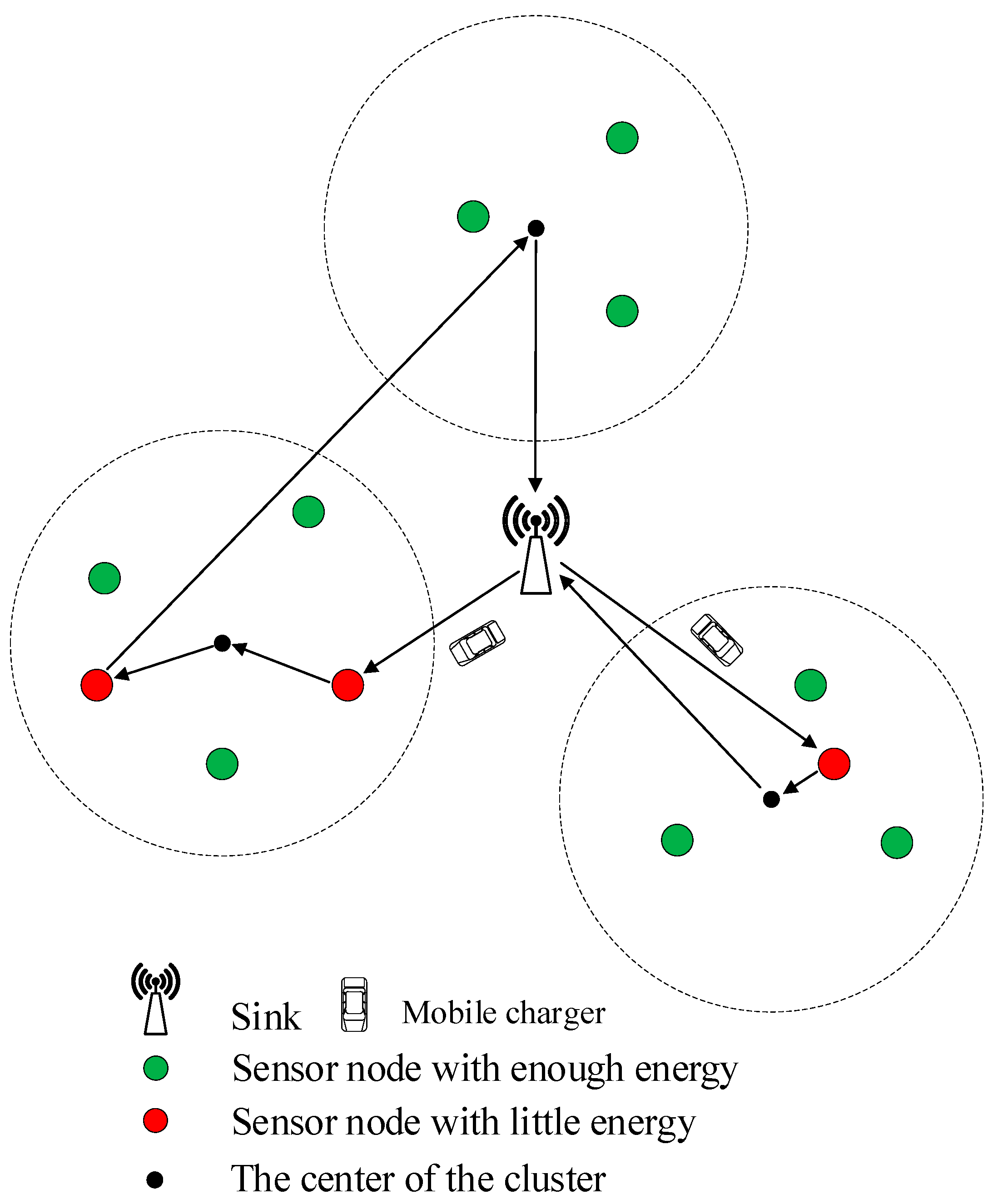
The network model of the new CRCM is shown in Figure 1. All sensor nodes are divided into three clusters. When the residual energy of some sensor nodes is lower than the threshold, these sensor nodes send charging requests to the sink by one-hop and multi-hop and then go into sleep mode. In this paper, we assumed that when the sensor node waits for the mobile charger’s arrival, the sensor node is in sleep mode without other activity. When the sink receives a certain number of charging requests, it dispatches several mobile chargers to serve the sensor nodes. The mobile charger is only dispatched to sensor nodes whose residual energy is lower than the charging threshold (shown in red in Figure 1). In this study, the mobile charger did not collect data directly from the sensor nodes when charging them. The centers of the clusters were added into each charging queue, and the mobile charger traveled to the centers of the clusters to gather all the sensing data from the sensor nodes in a cluster. The data acquisition cycle was set to make sure that all sensing data should be gathered in a certain time. When one mobile charger could not finish all tasks within the limited data acquisition cycle, multiple mobile chargers were needed. Sometimes, after a long time, the sensor nodes do not need to be charged, but we still arranged for mobile chargers to gather data.
3.2. Network Model of the New CRCM
In the new CRCM, the data transmission distance was within the single-hop distance. Therefore, we only discussed the Free Space Model to structure the sensor node energy consumption model as follows [30]:
where is the energy consumption for 1 bit data transmission in the Free Space Model. The communication distance is from the sensor node to the center of cluster . represents the energy consumption in the transmitting circuit when dealing with 1 bit data information. is the energy consumption of the power amplifier transmitting 1 bit data information to a unit area in the Free Space Model. The should be less than the single-hop correspondence distance , or else it will not satisfy the restriction of the Free Space Model. The value of can be calculated by Equation (2):
where represents the height of the transmitting antenna and is the height of the receiving antenna. is the transmission loss, and in the Free Space Model, the value of is two. is the energy consumption of the power amplifier transmitting 1 bit data to a unit area in the Multipath Fading Model, and in this paper, its value was . Since the value of was , the longest single-hop distance was calculated as 87.7 m.
3.3. Model of Mobile Charger Energy Consumption
When the mobile charger arrives at a sensor node, the service time for charging is calculated by Equation (3):
where represents the time taken to charge sensor node . is the time taken for the mobile charger to arrive at sensor node . represents the residual energy when the sensor node sends the charging request to the sink. As the mobile charger is traveling to the sensor node , the node continues to operate at a low energy consumption rate for a time ; the residual energy can be calculated by , and the energy that needs to be recharged can be calculated by . Since the charging power rate is and the charging efficiency is , the service time can be easily calculated.
When the mobile charger arrives at the centers of the clusters, it collects data from each node one at a time. Then, Equation (4) is used to define the service time of the cluster center :
where represents the time taken to collect data at the center of cluster , and is the time taken for one sensor node to transmit its data. Thus, the total time required to collect data is the sum of the times required for each sensor node in a cluster to transmit its data.
Next, we discuss the waiting time for the sensor node and the center of the cluster. In this paper, to ensure the data acquisition cycle, the data was gathered during each charging cycle. Thus, the centers of clusters were added into the charging queue. The mobile charger only traveled to sensor nodes to finish the task of charging, and then traveled to the center of the clusters to collect all sensing data. We defined as the time taken for the mobile charger to travel to the sensor nodes and define as the waiting time taken for the mobile charger to travel to the cluster centers, as follows:
For the sensor nodes which need to be served, if the former service object of the sensor node is also the sensor node, the waiting time model can be defined by Equation (5), where is the waiting time of the former sensor node , is the service time of the former sensor node , and is the distance between the sensor node and the former sensor node . The time taken for the mobile charger to move from the former sensor node to the sensor node can be calculated by , and the sum of these is the waiting time for the sensor node . If the former service object of the sensor node is the center of cluster , then the waiting time model can be defined by Equation (6). Since the former service object is the center of the cluster, the mobile charger only finishes the task of gathering data, and is the service time. is the time taken for the mobile charger to arrive at center . The is the time taken for the mobile charger to travel from center to sensor node .
Similarly, the time taken for the mobile charger to arrive at center also contains two conditions. Equations (7) and (8) can be explained in the same way.
4. Proposed Strategy
4.1. Clustering of the New CRCM
The consumption model of the sensor nodes and the mobile charger was structured in the same way as the system model of the new CRCM. We now discuss the methods of clustering to ensure that all the sensor nodes can be exactly divided into different clusters. In this paper, we used a K-means algorithm to partition the sensor nodes by the distance between the nodes and the cluster center. The most important parameter in this study was the number of clusters, K. In addition, by controlling the size of K, the size of the clusters can be limited to a single-hop range. Moreover, in this paper we only discussed the square area.
In fact, the number of clusters calculated by Equation (9) was an estimated value. The single-hop distance calculated in Equation (2) was 87.7 m. However, in this paper, we restricted the single-hop distance to within 50 m; then, as the area of the region increased, the number of clusters also increased. The area of the region was the main determinant of the value of , and as the number of sensor nodes increased, the original value of became unsuitable. We considered to ensure that when the number of sensor nodes was lower than 200 (experimental data), the value of would not decrease, and that when the number of sensor nodes was larger than 200, the value of would increase.
For example, if the length of the region, , is set as 100, and the number of sensor nodes, , is 100, then the value of can be calculated as . If is 300, then is calculated as . When is 200 and is 250, then can be calculated as .
4.2. Planning the Charging Path
During a charging cycle, some sensor nodes send requests to the sink node; these sensor nodes are then added into the service queue, . At the same time, since the data should be collected periodically, the centers of the clusters should also be added into the service queue. When the service queue is established, the sink node then dispatches several mobile chargers to finish the tasks of charging and data gathering. The movement path of a mobile charger is very important to the service efficiency of the mobile charger. In this paper, we took into account the distance to the mobile charger. Equation (10) is put forward to assist in the choice of the distance priority of the sensor node or the center of the cluster.
Since the movement path of the mobile charger starts from the sink, the first element of the queue is set as the sink node. The value of is always lower than 1, since the longest distance moved is always shorter than . As the distance moved increases, the also increases.
Path planning using Equation (10) is similar to the NJNP algorithm [17]—the first sensor node to be served is found next to the nearest node to the sink node, then the next sensor node is next to the nearest node to the first sensor node. As all elements are sorted, the reasonable queue is prototyped.
4.3. Periodically Restricted Dynamic Mobile Chargers
As the moving path for a single mobile charger is established, the service time for the mobile charger can be too long, such that the data cannot be gathered within a certain time period. Thus, we proposed the PRDMC algorithm to cut the original moving path to calculate the number of mobile chargers needed, then all sensor nodes’ data could be collected within a certain amount of time. If there is a situation in which no sensor nodes need to be charged for a long period of time, the PRDMC also arranges mobile chargers to visit the centers of clusters to gather data.
Unlike the single-hop and multi-hop data transmission methods, the data acquisition cycle contains two parts: free time and service time. Free time is the time in which the sink does not dispatch any mobile chargers to charge the sensor nodes. It is also the interval time of the charging cycles. We used to describe free time. The service time is the length of the charging cycle, and we defined it as . The data acquisition cycle can be defined as . In this paper, we considered data from 300 (experimental data) rounds as valid. We also limited the free time to 150 (experimental data) rounds.
Once a charging cycle starts, if the sink node only arranges one mobile charger to serve all sensor nodes, the service time of the whole queue can be calculated using Equation (11) and Equation (12):
where the sensor node or the center of the cluster is the last element in the queue . We defined the storage time as ; it determines the start time of the charging cycle. For example, if the sink only received a charging request from a sensor node, the calculated is less than the set value, so the sink continues to wait until more charging requests have been received. When is higher than the set value, the sink then calculates the number of mobile chargers and starts the charging cycle.
Another restrictive condition is the service time of mobile chargers. Regarding the sleep mode, once the sensor nodes are sent the charging requests, they then enter low power mode, and their residual times become longer. If the time limit of data acquisition is not considered, the can cause to be larger than 300. As a result, the sensing data is no longer valid. Hence, we use the following Equation (13) to limit the length of the charging cycle:
At the beginning of the charging cycle, when is lower than 150, must be larger than the set value, and the is also larger than 150, which means that one mobile charger can serve more sensor nodes. If reaches 150, there are two possible situations. One is that, if the is zero, it means that no sensor nodes need to be recharged; however, the sink still dispatches the mobile chargers to collect data. The other possible situation is that if the is larger than zero but the value of has not reached the set value, the sink still dispatches the mobile chargers to finish the tasks of charging and data collection.
In summary, due to the sleep mode and the length-limited charging cycle, we did not consider the lifetime of the sensor nodes. Actually, all of the sensor nodes were waiting for the arrival of the mobile chargers. We only cut the queue, , by the service time . At the same time, to improve the service efficiency of the mobile chargers, the storage time was set to determine the start time of the charging cycle. The charging strategy was distinct for different values of . When the was set to 0, the network model was that once one sensor node sent a charging request, the sink would dispatch a mobile charger to charge it. When the value of was set to infinity, the free time reached 150, and the sink node then arranged mobile chargers to serve the network. In this paper, we set the value of to 400, and the simulation results indicated that the number of mobile chargers is smaller and the service time is larger.
In order to further optimize the service efficiency of the charging vehicles, we next considered the service length of each mobile charger. The queue was cut by the condition of . The value of was changed with the value of the free time . We defined as the approximate number of mobile chargers:
where is the fractional part of ; when was less than 0.7, we considered that a very small number of sensor nodes were served by a mobile charger, and the service time was far smaller than for other mobile chargers. To solve this problem, we determined the number of mobile chargers using Equation (16):
Additionally, the extra time after cutting can be calculated by Equation (17):
For each additional mobile charger, there will be time for the mobile charger to travel to the sensor node and for its return to the sink. The longest time that the mobile charger takes to travel to the sensor node is . Then, the new restrictive condition can be calculated by Equation (18):
The detailed algorithm flow is shown below.
The sixth line in Algorithm 1 is used to judge the beginning of the charging cycle. Lines 12 to 14 are used to optimize the charging efficiency of each mobile charger. Then, these sensor nodes are added into the service queue of a mobile charger as the current elements meet the requirements. Once the service time of the mobile charger is larger than , the sensor nodes that have joined the mobile charger service queue are removed from the queue. Then, another mobile charger is set to repeat the previous operations. While all sensor nodes are removed from the queue, the number of mobile chargers is calculated, as is the service path of each mobile charger.
| Algorithm 1. The Periodically Restricted Dynamic Mobile Chargers (PRDMCs) algorithm. |
| 1: Input: The queue , count number , and length of |
| 2: Output: The number of mobile chargers |
| 3: |
| 4: |
| 5: let be the length of |
| 6: if or then |
| 7: |
| 8: for All do |
| 9: Calculate the waiting times and |
| 10: end for |
| 11: Calculate the |
| 12: if then |
| 13: |
| 14: end if |
| 15: while do |
| 16: if then |
| 17: |
| 18: else |
| 19: Remove the elements from 2 to and update the |
| 20: |
| 21: |
| 22: update the |
| 23: for All do |
| 24: Calculate the waiting times and |
| 25: end for |
| 26: end if |
| 27: if then |
| 28: |
| 29: end if |
| 30: end while |
| 31: end if |
| 32: Return: |
5. Simulations
5.1. Simulation Parameters
As shown in Table 2, the number of sensor nodes was set as 50, and the size of the region was . Each sensor node had an initial energy of . and when its residual energy was less than , it then sent a charging request to the sink.
5.2. Distribution and Clustering of Sensor Nodes
In order to obtain a clear presentation of the node distribution and the clustering, we set the number of sensor nodes to 50. From Figure 2, it can be seen that the sensor nodes were randomly positioned in the region.
5.3. Residual Energy of One Sensor Node
In this paper, the sensor nodes sent charging requests once, and then entered sleep mode to prolong their residual time. From Figure 3, it can be seen that the initial residual energy of the sensor nodes was . After their residual energy fell below , they sent a charging request to the sink and then went into sleep mode. In the new CRCM, the energy consumption after entering sleep mode was obviously lower than the original energy consumption. After the arrival of the mobile charger at each sensor node, the node was recharged and then returned to normal operation. The residual energy of the sensor node was charged regularly and periodically. As a result of the storage time that was set in the new CRCM, once the sink received a charging request, it would not dispatch mobile chargers at the same time. Therefore, it can be seen that the arrival time of the mobile charger in the new CRCM was later than that in the normal CRCM.
5.4. Number of Mobile Chargers Used in Each Charging Cycle
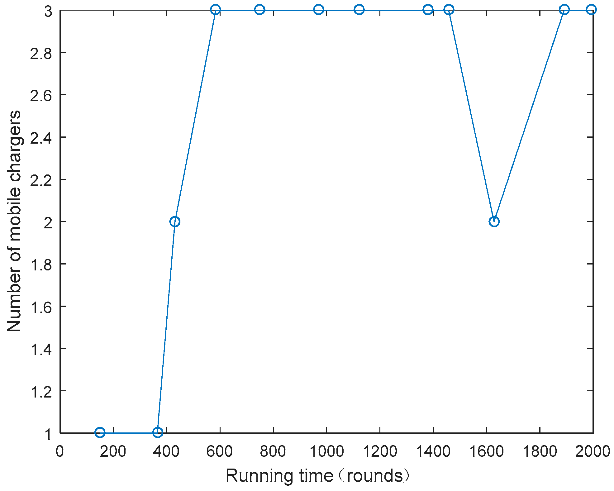
The number of mobile chargers used differs for different charging cycles. The number is determined based on the number of sensor nodes that need to be charged at the same time. From Figure 4, it can be seen that the number of mobile chargers changed irregularly. In the first two charging cycles, since there were no sensor nodes that needed to be charged, the free time was 150, and the sink node only dispatched one mobile charger to finish the task of gathering sensing data. After the network had ran for a period of time, several sensor nodes needed to be charged, and the number of mobile chargers was consequently increased.
5.5. Charging Path of Mobile Chargers
As previously mentioned, each mobile charger completes two tasks simultaneously, namely, charging and data gathering. In each charging cycle, if existing sensor nodes need to be charged, the mobile charger should complete both tasks. However, if no sensor nodes need to be charged, the mobile charger only finishes the task of data gathering. In the charging cycle scenario shown in Figure 5, no sensor nodes need to be charged, so the mobile charger only moves to the centers of clusters to collect sensing data from sensor nodes.
Figure 6 shows the original queue before cutting. It is the path of the closest principle choice. From Figure 6, it can be seen that the centers of the clusters were added into the charging path.
As a result of the storage time and the limited service time, one mobile charger alone cannot satisfy the charging requirement. In the scenario shown in Figure 7, three mobile chargers were dispatched.
5.6. Average Service Time of Mobile Chargers in Each Charging Cycle
In the normal CRCM, once a sensor node sends a charging request, the sink node then arranges one mobile charger to charge it. Without considering the data acquisition cycle, the servicing time of the mobile charger can be longer. Conversely, in the new CRCM, the storage time and the limited service time mean that the service time of the mobile chargers must be within a certain range. As can be seen from Figure 8, there are eight charging cycles in the normal CRCM. In the new CRCM, there are 11 charging cycles, and in the first two charging cycles, the service time is equal, as the mobile chargers only finish the task of data gathering. The service time of mobile chargers in the new CRCM is always lower than in the normal CRCM. Though the charging efficiency of mobile chargers in the new CRCM is lower than in the normal CRCM, data acquisition cycle is nevertheless guaranteed.
5.7. Length of Storage Time
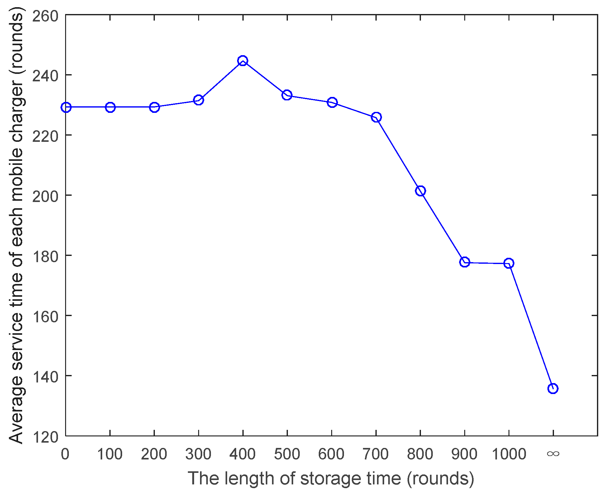
The storage time is set to increase the service efficiency of each mobile charger. When the length of the storage time is equal to 0, once the sink has received a charging request, it then sends a mobile charger to charge the sensor node. The service efficiency of the mobile chargers is very low. When is infinite, the free time is always 150, and due to the limit of the data acquisition cycle, the service time of each mobile charger cannot exceed 150 cycles. Obviously, the number of mobile chargers will be larger. From Figure 9 and Figure 10, it can be seen that, when is equal to 400, the number of mobile chargers is smallest, and the service time of each mobile charger is largest. Therefore, in this paper, we set to 400.
5.8. Average Data Gathering Cycle
The normal CRCM only ensures that the sensor nodes do not break out. Once a mobile charger arrives at a sensor node, it simultaneously charges the node and gathers its sensing data. Therefore, the data gathering cycle of one sensor node can be considered as the interval time of the mobile charger’s arrival. From Figure 11, it can be seen that as the number of senor nodes increased, the average length of the data gathering cycle in the normal CRCM was stable. Before the energy consumption of the node is exhausted, the mobile charger must travel to the node to charge it, so the data acquisition cycle will not change much. In the new CRCM, all sensor nodes are divided into several clusters, and the mobile chargers only travel to the centers of the clusters to finish the task of data gathering. The data gathering cycle in the new CRCM is much shorter than in the normal CRCM, and it is stable with increasing numbers of sensor nodes. This is due to the fact that the data gathering time is limited in the new CRCM, and the principle of cutting the charging queue of each mobile charger is in strict accordance with the service time .
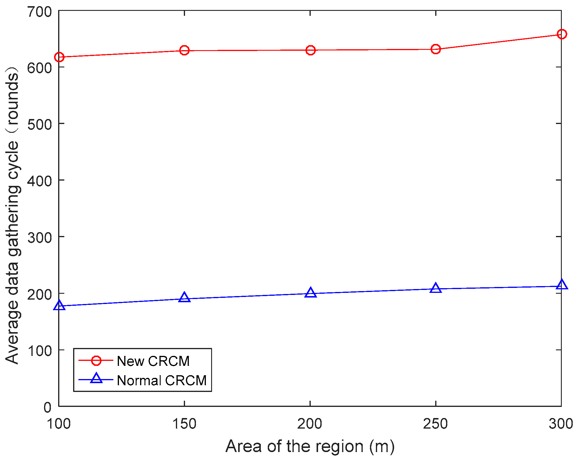
Figure 12 shows the change in the average length of the data gathering cycle with increasing region size. In both the normal CRCM and the new CRCM, the data gathering time was always stable, and in the new CRCM, the data acquisition cycle was guaranteed.
5.9. Average Number of Mobile Chargers Used in Each Charging Cycle
In the new CRCM, the sleep mode clearly improved the charging efficiency of the mobile chargers. In the normal CRCM, the queue is cut by the residual lifetime of the sensor nodes. This will result in some mobile chargers only serving several sensor nodes. However, in the new CRCM, the sleep mode increased the lifetime of each sensor node, and queue was only cut by the service time , then, by optimizing the efficiency of the mobile charger in the PRDMC, the average number of mobile chargers in the new CRCM was lower than in the normal CRCM. Figure 13 and Figure 14 show the change in the average number of mobile chargers in each charging cycle with increasing numbers of sensor nodes and increasing region size, respectively. From Figure 14, it can be seen that the new CRCM always performed better than the normal CRCM.
6. Conclusions
In the new CRCM, the tasks of data gathering and node charging were achieved asynchronously by mobile chargers. The mobile chargers moved close to sensor nodes and recharged them wirelessly. Then, the chargers travelled to the center of each cluster to collect data from the sensor nodes. In order to extend their survival time until the mobile charger arrives, sensor nodes enter sleep mode as they send charging requests to the sink. To achieve reasonable clustering, we determined the number of clusters using a K-means algorithm. As the centers of each cluster were added into the charging queue, the NJNP algorithm was used to optimize the charging route. The PRDMC algorithm was proposed to calculate the number of mobile chargers to solve two problems regarding how to ensure that data can be collected within a specified time period when there are sensor nodes that need to be recharged, and how to ensure that data can be collected within a specified time period when there are no sensor nodes that need to be charged. Using simulations, we found that the data acquisition cycle was guaranteed in the new CRCM without adding too many mobile chargers.
Author Contributions
Conceptualization, Y.W. and Y.D.; Methodology, Y.W.; Software, Y.W.; Validation, Y.W., Y.D. and S.L.; Formal Analysis, Y.W.; Investigation, R.H.; Resources, Y.D.; Data Curation, Y.S.; Writing—Original Draft Preparation, Y.W.; Writing—Review and Editing, Y.W. and Y.D.; Visualization, Y.W.; Supervision, Y.D.; Project Administration, Y.W.; Funding Acquisition, Y.D.
Funding
This research was sponsored by the National Natural Science Foundation of China (No. 61107040) and Science and Technology Department of Jilin Province (No. 0180101042JC).
Conflicts of Interest
The authors declare no conflict of interest.
References
- García-Hernández, C.F.; Ibarguengoytia-Gonzalez, P.H.; García-Hernández, J.; Pérez-Díaz, J.A. Wireless sensor networks and applications: A survey. Int. J. Comput. Sci. Netw. Secur. 2007, 7, 264–273. [Google Scholar]
- Yick, J.; Mukherjee, B.; Ghosal, D. Wireless sensor network survey. Comput. Netw. 2008, 52, 2292–2330. [Google Scholar] [CrossRef]
- Jing, Q.; Vasilakos, A.V.; Wan, J.; Lu, J.; Qiu, D. Security of the Internet of Things: Perspectives and challenges. Wirel. Netw. 2014, 20, 2481–2501. [Google Scholar] [CrossRef]
- Pan, J.S.; Dao, T.K. A Novel Improved Bat Algorithm Based on Hybrid Parallel and Compact for Balancing an Energy Consumption Problem. Information 2019, 10, 194. [Google Scholar] [CrossRef]
- Chen, J.; Hu, K.; Wang, Q.; Sun, Y.; Shi, Z.; He, S. Narrow-Band Internet of Things: Implementations and Applications. IEEE Internet Things J. 2017, 4, 2309–2314. [Google Scholar] [CrossRef]
- Casares-Giner, V.; Navas, T.I.; Flórez, D.S. End to End Delay and Energy Consumption in a Two Tier Cluster Hierarchical Wireless Sensor Networks. Information 2019, 10, 135. [Google Scholar] [CrossRef]
- Yang, Y.Y.; Wang, C. Wireless Rechargeable Sensor Networks; Springer: Berlin/Heidelberg, Germany, 2015; pp. 1–53. [Google Scholar]
- Ren, P.; Wang, Y.; Du, Q. CAD-MAC: A Channel-Aggregation Diversity Based MAC Protocol for Spectrum and Energy Efficient Cognitive Ad Hoc Networks. IEEE J. Sel. Areas Commun. 2014, 32, 237–250. [Google Scholar]
- Zhang, J.; Wu, C.; Zhang, Y.; Ji, P. Energy-efficient Adaptive Dynamic Sensor Scheduling for Target Monitoring in Wireless Sensor Networks. ETRI J. 2011, 33, 857–863. [Google Scholar] [CrossRef]
- Luo, J.; Panchard, J.; Piórkowski, M.; Grossglauser, M.; Hubaux, J.P. MobiRoute: Routing Towards a Mobile Sink for Improving Lifetime in Sensor Networks. In Distributed Computing in Sensor Systems; Springer: Berlin/Heidelberg, Germany, 2006. [Google Scholar]
- Nitesh, K.; Azharuddin, M.; Jana, P.K. A novel approach for designing delay efficient path for mobile sink in wireless sensor networks. Wirel. Netw. 2018, 24, 2337–2356. [Google Scholar] [CrossRef]
- Tong, B.; Li, Z.; Wang, G.; Zhang, W. How Wireless Power Charging Technology Affects Sensor Network Deployment and Routing. In Proceedings of the 2010 International Conference on Distributed Computing Systems (ICDCS 2010), Genova, Italy, 21–25 June 2010. [Google Scholar]
- Kansal, A.; Hsu, J.; Zahedi, S.; Srivastava, M.B. Power management in energy harvesting sensor networks. ACM Trans. Embed. Comput. Syst. 2007, 6, 32. [Google Scholar] [CrossRef]
- Xie, L.; Shi, Y.; Hou, Y.T.; Lou, W.; Sherali, H.D. On traveling path and related problems for a mobile station in a rechargeable sensor network. In Proceedings of the Fourteenth ACM International Symposium on Mobile Ad Hoc Networking & Computing, Bangalore, India, 29 July–1 August 2013. [Google Scholar]
- He, L.; Gu, Y.; Pan, J.; Zhu, T. On-demand Charging in Wireless Sensor Networks: Theories and Applications. In Proceedings of the 2013 IEEE 10th International Conference on Mobile Ad-Hoc and Sensor Systems, Hangzhou, China, 14–16 October 2013. [Google Scholar]
- Zhao, L.; Tang, Q. An Improved Threshold-Sensitive Stable Election Routing Energy Protocol for Heterogeneous Wireless Sensor Networks. Information 2019, 10, 125. [Google Scholar] [CrossRef]
- He, L.; Kong, L.; Gu, Y.; Pan, J.; Zhu, T. Evaluating the On-Demand Mobile Charging in Wireless Sensor Networks. IEEE Trans. Mob. Comput. 2015, 14, 1861–1875. [Google Scholar] [CrossRef]
- Wang, Y.; Dong, Y.; Li, S.; Wu, H.; Cui, M. CRCM: A New Combined Data Gathering and Energy Charging Model for WRSN. Symmetry 2018, 10, 319. [Google Scholar] [CrossRef]
- Hartigan, J.A.; Wong, M.A. Algorithm AS 136: A K-Means Clustering Algorithm. J. R. Stat. Soc. 1979, 28, 100–108. [Google Scholar] [CrossRef]
- Fragkiadakis, A.; Askoxylakis, I.; Tragos, E. Joint compressed-sensing and matrix-completion for efficient data collection in WSNs. In Proceedings of the IEEE International Workshop on Computer Aided Modeling & Design of Communication Links & Networks, Berlin, Germany, 25–27 September 2013. [Google Scholar]
- Al-Baz, A.; El-Sayed, A. A new algorithm for cluster head selection in LEACH protocol for wireless sensor networks. Int. J. Commun. Syst. 2017, 31, e3407. [Google Scholar] [CrossRef]
- Açıcı, K.; Erdaş, Ç.; Aşuroğlu, T.; Oğul, H. HANDY: A Benchmark Dataset for Context-Awareness via Wrist-Worn Motion Sensors. Data 2018, 3, 24. [Google Scholar] [CrossRef]
- Gambhir, S. OE-LEACH: An optimized energy efficient LEACH algorithm for WSNs. In Proceedings of the Ninth International Conference on Contemporary Computing, Noida, India, 11–13 August 2016. [Google Scholar]
- Xiangning, F.; Yulin, S. Improvement on LEACH protocol of wireless sensor network. In Proceedings of the 2007 International Conference on Sensor Technologies and Applications (SENSORCOMM 2007), Valencia, Spain, 14–20 October 2007; pp. 260–264. [Google Scholar]
- Yun, Y.S.; Xia, Y. Maximizing the Lifetime of Wireless Sensor Networks with Mobile Sink in Delay-Tolerant Applications. IEEE Trans. Mob. Comput. 2010, 9, 1308–1318. [Google Scholar]
- Nguyen, T.D.; Chu, S.I.; Liu, B.H.; Chen, C.H.; Dang, H.S.; Perumal, T. Mobile charging and data gathering in multiple sink wireless sensor networks: How and why. In Proceedings of the International Conference on System Science & Engineering, Ho Chi Minh City, Vietnam, 21–23 July 2017. [Google Scholar]
- Lin, C.; Xue, B.; Wang, Z.; Han, D.; Deng, J.; Wu, G. DWDP: A Double Warning Thresholds with Double Preemptive Scheduling Scheme for Wireless Rechargeable Sensor Networks. In Proceedings of the Neural Information Processing Systems, New York, NY, USA, 24–26 August 2015; pp. 1515–1522. [Google Scholar]
- Lin, C.; Wang, Z.; Han, D.; Wu, Y.; Yu, C.W.; Wu, G. TADP: Enabling temporal and distantial priority scheduling for on-demand charging architecture in wireless rechargeable sensor Networks. J. Syst. Archit. 2016, 70, 26–38. [Google Scholar] [CrossRef]
- Liu, B.H.; Nguyen, N.T.; Pham, V.T.; Lin, Y.X. Novel methods for energy charging and data collection in wireless rechargeable sensor networks. Int. J. Commun. Syst. 2017, 30, e3050. [Google Scholar] [CrossRef]
- Aernouts, M.; Berkvens, R.; Van Vlaenderen, K.; Weyn, M. Sigfox and LoRaWAN Datasets for Fingerprint Localization in Large Urban and Rural Areas. Data 2018, 3, 13. [Google Scholar] [CrossRef]
Figure 1.
A diagram of the Wireless Rechargeable Sensor Network (WRSN) mode.

Figure 2.
Distribution and clustering of the sensor nodes. The four black diagonal crosses are the centers of each cluster. The black horizontal cross in the middle of the region is the sink node. The dotted lines indicate node–mobile charger data transfer that is performed when the mobile charger arrives at the center of the cluster.

Figure 3.
Residual energy of one sensor node.

Figure 4.
Number of mobile chargers used in each charging cycle.

Figure 5.
The charging path of a mobile charger while completing data gathering.

Figure 6.
The original charging path of a mobile charger before cutting, the blue stars represent sensor nodes that need to be charged in the present charging cycle.
Figure 6.
The original charging path of a mobile charger before cutting, the blue stars represent sensor nodes that need to be charged in the present charging cycle.

Figure 7.
Charging paths of multiple mobile chargers. The differently colored lines represent the driving paths of different mobile chargers.
Figure 7.
Charging paths of multiple mobile chargers. The differently colored lines represent the driving paths of different mobile chargers.

Figure 8.
Average service time of mobile chargers for two CRCMs (Combined Recharging and Collecting Data Model).
Figure 8.
Average service time of mobile chargers for two CRCMs (Combined Recharging and Collecting Data Model).

Figure 9.
Number of mobile chargers for different lengths of storage time.

Figure 10.
Average service time of each mobile charger for different lengths of storage time.

Figure 11.
Average length of the data gathering cycle for two CRCMs.

Figure 12.
Average length of the data gathering cycle for different region sizes.

Figure 13.
Average number of mobile chargers for different numbers of sensor nodes.

Figure 14.
Average number of mobile chargers for different region sizes.


Table 1.
Symbol and definitions.
| Symbol | Definition |
|---|---|
| sensor node | |
| the center of cluster | |
| the length of the region | |
| charging threshold | |
| the initial energy of each sensor node | |
| the charging efficiency of the mobile charger | |
| the charging power of the mobile charger | |
| the residual energy of sensor node when sending a charging request to the sink | |
| the energy consumption of sensor node | |
| the charging time for sensor node | |
| the time required for the mobile charger to leave sensor node | |
| the time required for data collection when the mobile charger is operating in the center of cluster | |
| energy consumption for 1 bit data transmission in the Free Space Model | |
| energy consumption in the transmitting circuit when dealing with 1 bit data information | |
| the time required for the mobile charger to leave cluster | |
| the time required to collect data from sensor node | |
| the number of clusters | |
| the data size of sensor node | |
| the increase in time after cutting the charging queue | |
| the number of mobile chargers | |
| the moving speed of the mobile charger | |
| the total time required for the charging queue | |
| the length of the storage time | |
| the service time of the mobile charger | |
| the interval time among two charging cycles |
Table 2.
Simulation parameters.
| Parameters | Value |
|---|---|
| Number of nodes | 50 |
| Field size (m2) | |
| Number of clusters | 4 |
| Initial energy of the node (KJ) | 0.5 |
| Energy consumption during communication per datum (nJ/bit) | 50 |
| Speed of the mobile charger (m/s) | 1 |
| Energy conversion rate of mobile chargers (ω) | 0.8 |
| Charging threshold (KJ) | 0.2 |
© 2019 by the authors. Licensee MDPI, Basel, Switzerland. This article is an open access article distributed under the terms and conditions of the Creative Commons Attribution (CC BY) license (http://creativecommons.org/licenses/by/4.0/).
Share and Cite
MDPI and ACS Style
Wang, Y.; Dong, Y.; Li, S.; Huang, R.; Shang, Y. A New on-Demand Recharging Strategy Based on Cycle-Limitation in a WRSN. Symmetry 2019, 11, 1028. https://0-doi-org.brum.beds.ac.uk/10.3390/sym11081028
AMA Style
Wang Y, Dong Y, Li S, Huang R, Shang Y. A New on-Demand Recharging Strategy Based on Cycle-Limitation in a WRSN. Symmetry. 2019; 11(8):1028. https://0-doi-org.brum.beds.ac.uk/10.3390/sym11081028
Chicago/Turabian StyleWang, Yuhou, Ying Dong, Shiyuan Li, Ruoyu Huang, and Yuhao Shang. 2019. "A New on-Demand Recharging Strategy Based on Cycle-Limitation in a WRSN" Symmetry 11, no. 8: 1028. https://0-doi-org.brum.beds.ac.uk/10.3390/sym11081028
Note that from the first issue of 2016, this journal uses article numbers instead of page numbers. See further details here.