Synthesis on the Acceleration Energies in the Advanced Mechanics of the Multibody Systems


Faculty of Machine Building, Department of Mechanical Systems Engineering, Technical University of Cluj-Napoca, 400641 Cluj-Napoca, Romania
*
Authors to whom correspondence should be addressed.
Symmetry 2019, 11(9), 1077; https://0-doi-org.brum.beds.ac.uk/10.3390/sym11091077
Submission received: 16 July 2019
/
Revised: 12 August 2019
/
Accepted: 22 August 2019
/
Published: 27 August 2019
(This article belongs to the Special Issue Symmetry in Applied Continuous Mechanics)
Abstract
:The present paper’s objective is to highlight some new developments of the main author in the field of advanced dynamics of systems and higher order dynamic equations. These equations have been developed on the basis of the matrix exponentials which prove to have undeniable advantages in the matrix study of any complex mechanical system. The present paper proposes some new approaches, based on differential principles from analytical mechanics, by using some important dynamics notions, regarding the acceleration energies of the first, second and third order. This study extended the equations of the higher order, which provide the possibility of applying the initial motion conditions in the positions, velocities and accelerations of the first and second order. In order to determine the time variation laws for the generalized variables, the driving forces and acceleration energies of the higher order are applied by the time polynomial functions of the fifth order. According to inverse kinematics also named control kinematics of the robots, the applications of polynomial functions lead to the kinematic control functions of mechanical motions, especially the transitory motions. They influence the dynamic behavior of multibody systems, in which robot structures are included.
1. Introduction
Until the present, the dynamic behavior of rigid body and of the multibody systems can be studied by considering the fundamental theorems from dynamics or the differential principles of analytical mechanics [1,2,3,4]. Both are based on angular momentum, the mechanical work and kinetic energy, as well as on their fundamental theorems. In mechanics, the defining expressions for the advanced notions are based on fundamental input parameters that are represented by kinematic parameters along with their differential transformations, as well as by the mass properties highlighted by the inertia tensor and corresponding generalized variation laws.
The advanced concepts include higher-order accelerating energies known in the scientific literature [5,6,7] as kinetic energies of higher-order accelerations. The kinetic energy is used, in Newtonian mechanics, as a central function of Lagrange Euler equations. The existence of higher-order accelerations has been proven by the fact that they occur every time the bodies/multi-body systems are subjected to fast and sudden motions or, when particularly, this type of excitation produces vibration modes with more frequencies of resonance. The acceleration itself cannot produce vibration being just a static load. In fact, the sudden motions are generated by higher order accelerations. For example, during the operation of a cam and cam follower mechanism at high speeds and accelerations, the jumping off of the cam follower from the camshaft causing accidents may occur. Another example is the case of manufacturing processes that require rapid changes in the acceleration of a cutting tool. This leads to a quick tool wear and results in poor quality of the manufactured surfaces [8,9]. The two situations presented above are generated by the effect of higher order accelerations. These effects have to be also considered each time when a mechanical system is in a transient motion phase (take-off/landing, acceleration/deceleration, etc.). The novelty of the paper consists in presenting a new approach regarding the dynamic modeling of rigid bodies and multibody mechanical systems. Based on scientific literature [10,11,12,13,14,15,16,17,18,19,20], the input kinematic and dynamic parameters have been formulated. These parameters are compulsorily included in the dynamic equations of the higher order, corresponding to fast and sudden motions. This type of motion characterizes the multibody systems, a category where the robots are also included. The important formulations regarding the acceleration energies of the first, second, third and higher orders are also presented in explicit and matrix forms. The expressions for the acceleration energies of the higher order were determined, among others, based on matrix exponential functions [14,19]. Although at first sight they seem difficult to put into practice, they proved to have undisputable advantages in terms of their use in the kinematic and dynamic study of complex mechanical systems.
These expressions are implemented into the differential equations of the higher order, thus resulting the time variations of the generalized forces, which influences the dynamic behavior of rigid body or of multibody systems. To illustrate the validity of the proposed mathematical model, an experimental study, in which the higher order accelerations are highlighted, is performed.
2. Input Parameters in Advanced Dynamic Modeling
2.1. Position and Orientation Parameters
In Newtonian mechanics, the dynamics of the rigid bodies are studied based on the assumption that they do not deform under the action of the external forces.
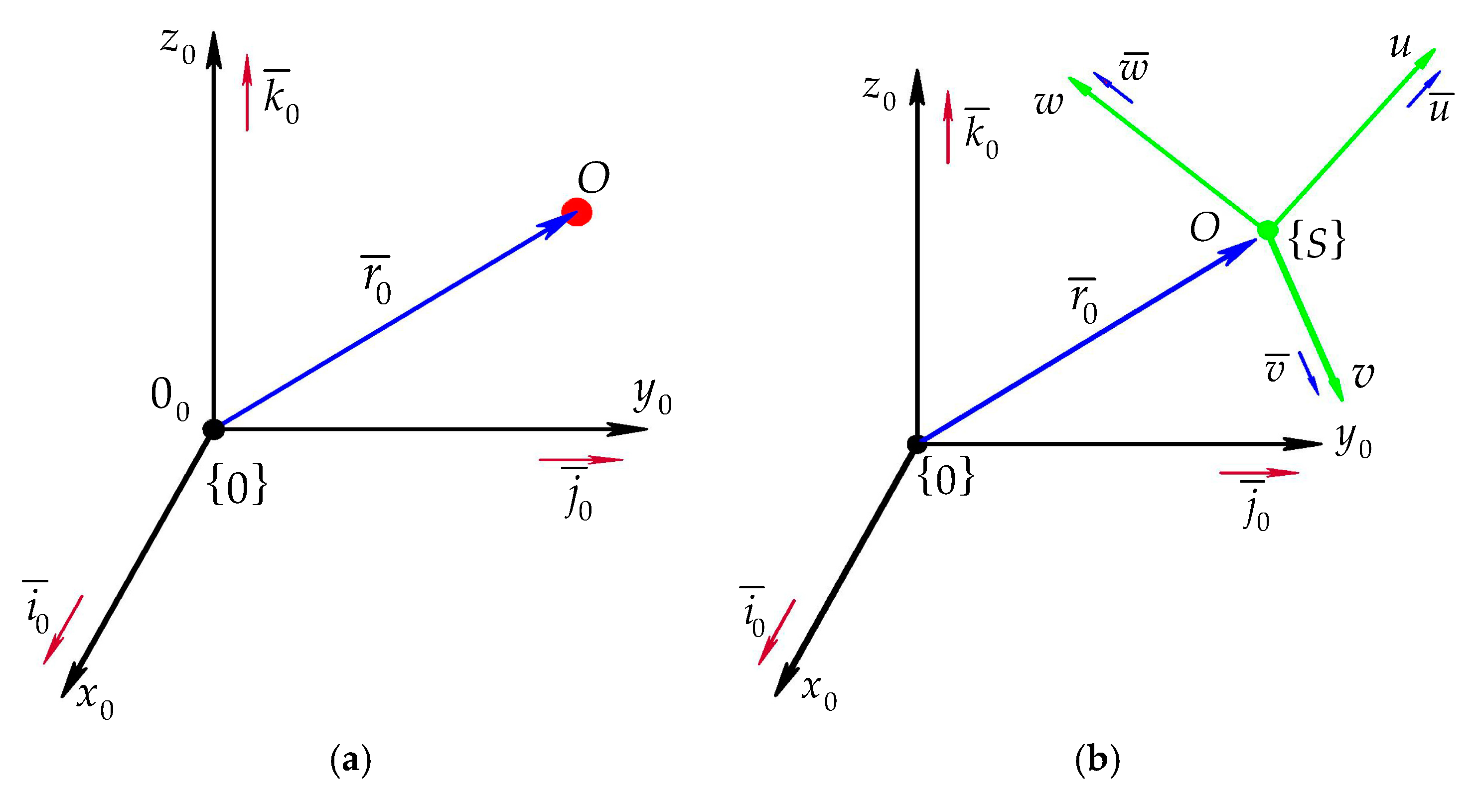
To study the dynamical behavior of a rigid body, its linear and angular position in the Cartesian space must be known at each moment during the motion. To define the linear and angular position, [13,20], the last one being also known as orientation, the simplest mechanical model, which is the material point, is analyzed (Figure 1).
The following notations are considered:
In the Expression (1), the coordinates or axes of the Cartesian frame, symbols from (2) representing the unit vectors, and (3) the angles and the direction cosines are defined.
The dynamic study of the rigid solid is carried out, according to Figure 1, by considering two reference systems: , which is considered fixed and which is a mobile reference system, invariably linked to the body, having the origin in an arbitrary point belonging to the rigid body. The system , represented in the same figure, is a system which originated in point , and whose orientation is maintained constant all throughout the movement and is identical with the orientation of the fixed system, , that is .
The geometrical state of any material point (for example a certain point ) characterizes the position, according to Figure 1a. The position is usually defined by means of the position vector:
The three linear coordinates from (5) are independent in the case of a free material point, and represents the degrees of freedom (d.o.f.). Further, the study is extended to a vector or an axis belonging to the Cartesian frame (see Figure 1b). This geometrical state is called orientation (angular position). Orientation (angular position) is defined through unit vectors. For any given unit vector , in relation to one of the frames /, the orientation is defined by the direction cosines:
According to linear algebra, in expression (6), the symbol defines the transposed matrix.
Further, considering the second expression from (6), the orientation of any vector or axis is characterized by two independent angles. The above geometrical aspects are extended on an orthogonal and right oriented frame (see Figure 1b, ) relative to . In this case, the geometrical state is defined by position and orientation. The position is defined by means of position vector (5), while for orientation the rotation matrix is considered [10]:
The resultant orientation matrix defined with (7), contains the unit vectors of frame relative to . The rotation matrix or the matrix of direction cosines describes the orientation of each axis of the mobile frame attached to the rigid body, relative to a fixed frame. Between the nine direction cosines contained by the rotation matrix, six mathematical relations can be established. Thus, the result is that the orientation of a mobile frame with respect to a fixed frame is defined by up to three independent parameters, which are defining the orienting angles. Therefore, the resultant orientation of a frame with respect to another frame, / is characterized by three independent orientation angles (three d.o.f), [13]:
The angles from (8) are the components of the column matrix of orientation , and they describe, from a geometrical point of view, dihedral angles between two geometrical planes:
Physically, the three angles defined with (8) expresses a simple rotation around one of the axes of the Cartesian reference system: . Based on research from [10,11,12,13,14], when combining the three simple rotations, there is a result of twelve sets of orientation angles (8). Taking , the expressions of definition are further developed for the three simple rotation matrices symbolized as:
The paper proposes the following form of mathematical representation for the generalized matrix:
By substituting (11) and (12) in the generalized expression (10), the simple rotation matrices (9) are obtained. The generalized matrix can be written in a new formulation as follows:
In the expression (13), the symbol defines the skew-symmetric matrix associated to (15), while represents the diagonal matrix, written below:
By applying (14) and (15), an expression identical with the classical Rodriguez formula is obtained [17]:
According to research from [3,4,5,6,7,8,9,10], the three simple rotations from (8) are performed either around the moving axes or fixed axes belonging to or /. The resultant rotation matrix, symbolized as , defines the orientation of the system ( attached to the rigid body), with respect to a fixed system , and is represented in the following matrix form:
Using the research in the field of matrix exponentials [10,14], the following form for the resultant rotation matrix (18) is written as:
The above mathematical Expressions (5) and (8), which define the position and orientation in the case of a rigid body, are written in a general form. Based on the definitions from the first paragraph of this section, a rigid body consists of an infinite number of material points and also, an infinite number of geometrical axes, parallel and perpendicular one to another, characterized by a continuous distribution in the entire volume of the rigid [14,15]. The rigid body is also made up of an infinite number of assemblies consisting of three orthogonal geometrical plans, continuously distributed in the entire volume of the rigid body.
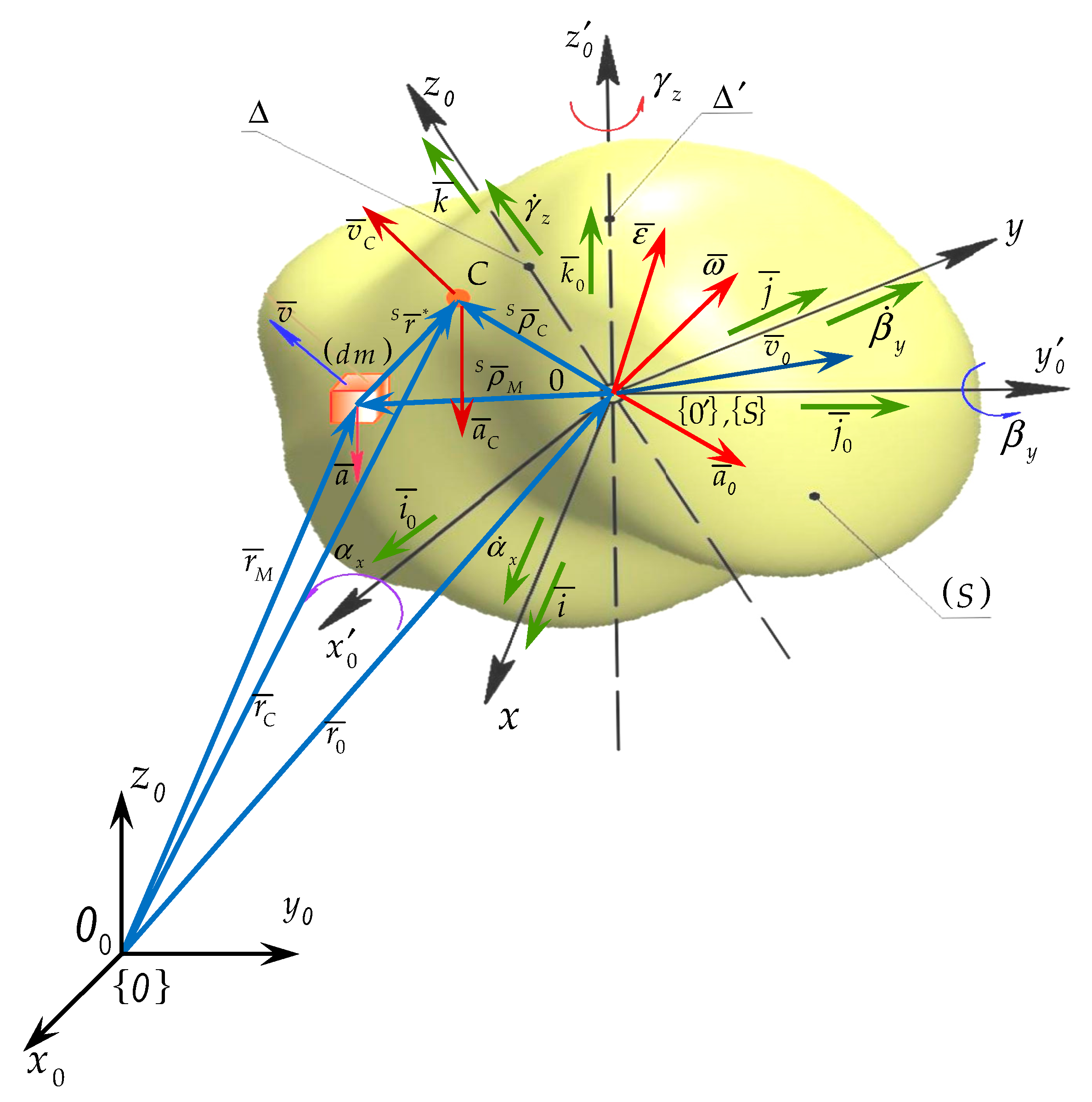
In terms of geometry, in order to define a right oriented reference frame having the origin in an arbitrary point of the rigid body, a single ensemble composed of three orthogonal geometrical plans is chosen. According to (4) and Figure 2, this reference frame is symbolized as . The reference frame is linked to the body due to its rigid nature. Expressions (5) and (8) define the position and orientation of this frame.
Whereas the present paper proposes a study on advanced dynamics, it considers two material points belonging to a rigid body, so that the following conditions are met: and . In this case, the expressions defining the position can be written as time functions, according to [12]:
Based on (18) and (19), the position equation is written, by considering the matrix exponentials:
The position equation for any material point from the rigid body can be determined only when the position and orientation of the moving frame are well known. By analyzing the Expressions (21) and (22), the result is that the orientation is invariant for all the points of the rigid solid. Thus, by considering the geometrical aspects, the body is substituted by the moving frame . This is defined from a geometrically point of view by means of the six independent parameters (six d.o.f.), which are included in the following symbol:
where is the generalized coordinate and is an operator which highlights the type of driving joint. In this paper, the symbol , is substituted as:
Considering Expression (24), the following notations are implemented:
where represents the order of the time derivative.
In advanced mechanics, instead of (8), in the case of the angular vector of orientation, the following expression of definition is used:
where represents the angular transfer matrix which is a function of the orienting angles.
In mechanics, the position and orientation of a moving frame , with respect to another frame, for example a fixed frame , is represented in a matrix form, according to [5,8] by means of homogeneous transformations which are developed using matrix exponentials:
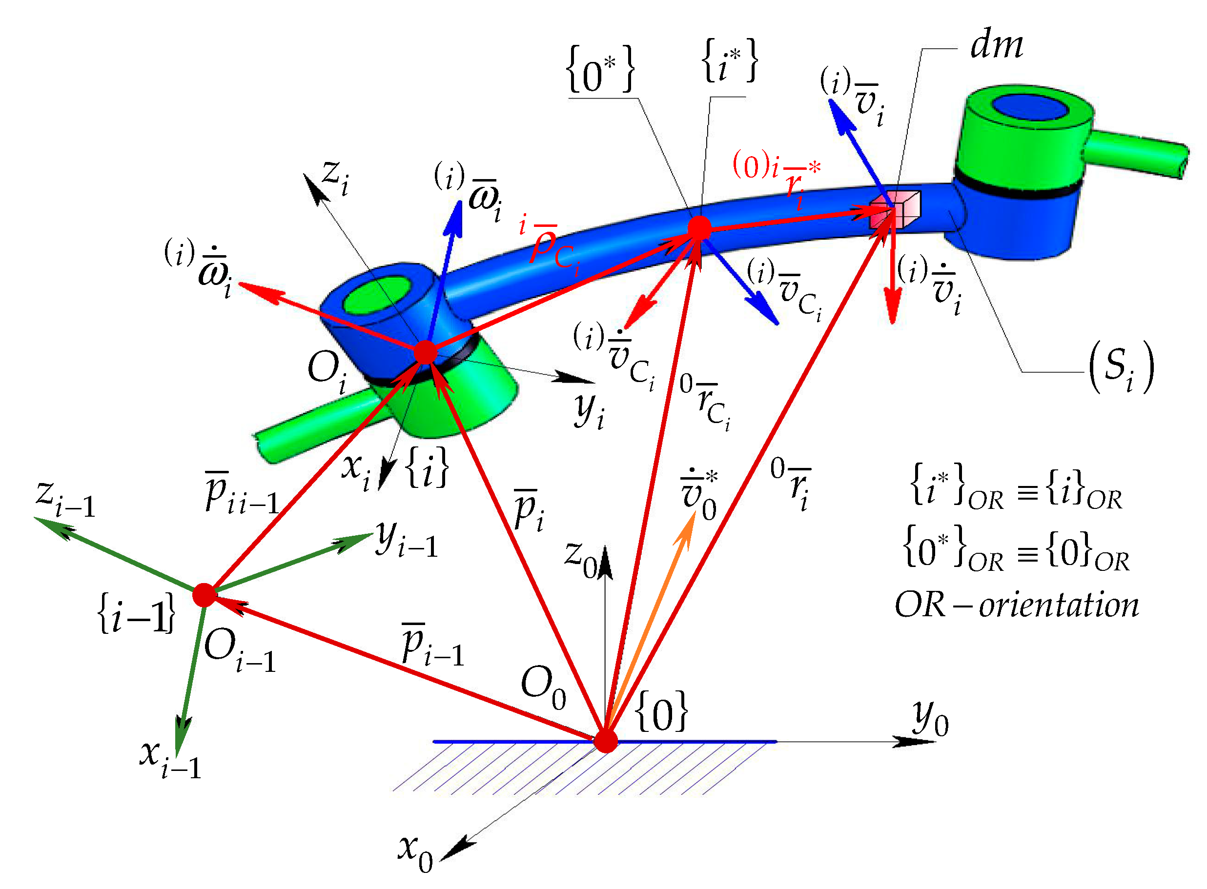
Expression (30) defines the position vector of the mobile system relative to fixed system , while (31) represents a position vector, which according to [11,20], is defined by means of homogenous coordinates as a function of screw parameters. The conclusions and expressions of definition, synthetically disseminated in this introductory section, are compulsory applied in the advanced kinematics and dynamics of mechanical systems. For example, a kinetic element from this mechanical structure of a robot is considered (Figure 3).
In case of both rigid bodies and multibody systems, the dynamical study of current and sudden motions is performed. The study is based on the differential principles from analytical dynamics of systems, as well as on the advanced notions from the dynamics of solid bodies: Momentum and angular momentum, kinetic energy, acceleration energies of different orders and their absolute time derivatives of the high order.
2.2. The Kinematic Parameters of Higher Order
The parametric equations of motion are defined according to (24). The absolute position Equation (21) shows the variable distribution from a point to another material point of the body. By applying the first order time derivative on Expression (21), the result is:
The following property is mandatory for the motion equations defined with (32):
where considering [1,10], is the skew symmetric matrix associated to the angular velocity vector.
The time derivatives of the higher order, applied on the property (32), are defined as follows:
In advanced kinematics and dynamics, the time derivatives of the higher order for rotation matrices and position vectors must be used according to [10,11,12,13] as follows:
The symbols: and represent the order of the time derivatives applied on expressions (35) and (36).
The expressions of definition for angular velocities, and then for the angular accelerations are:
By analyzing (38), it is noticed that the expressions of the kinematic parameters that define the resultant rotation motion are written based on the matrix exponential functions.
Both velocities and accelerations of the higher order are established based on the following vectors:
where the orientation vector is defined according to the following expressions: (8), (19), (27) and (28).
An essential component (28) included in (40), known as the angular transfer matrix, can be defined as a function of a set of the orientation angles. Considering (39) and (40), it is observed that they are functions of generalized variables (24) and (25). Actually, the six generalized variables are the independent parameters of the position and orientation from (24). Using the research from [10,11,12,13,14], the on-time functions associated to position (39) and orientation (40) vectors and the differential properties which are compulsory and applied in advanced kinematics and dynamics, have been developed:
The symbols and from (41) and (42) define the deriving orders with respect to time.
The expression (44) defines the angular and linear accelerations of the higher order for a rigid solid in general motion. The input expressions and parameters of the higher order are compulsory and applied in the definition of the dynamic notions of the higher order, such as the momentum, angular momentum, kinetic energy and acceleration energy of the higher order.
They have been included in the dynamics theorems which applies to current and sudden motions.
The next step consists of establishing the time variation law for the generalized coordinates and generalized variables of the higher order. Considering [9], the result is that all parameters from advanced kinematics are functions of generalized variables as well as of their time derivatives and they can be developed by using polynomial interpolation functions [13,20]. The following general form for the polynomial interpolation functions of the higher order is used:
For every trajectory interval , the number of unknowns is , and their significance is:
To determine the unknowns, (50) is required to apply geometrical and kinematical constraints:
The kinematical constrains that can be applied in the case of polynomials of the higher order are:
Finally, Expression (45) is substituted in the advanced notions of kinematics and dynamics.
2.3. The Mass Properties
In order to find an exact geometrical solution, it is considered that the rigid body consists of an infinite number of material particles for which the distance between two points is maintained constant, regardless of the forces that act upon it. The elementary particles, characterized by elementary and infinitesimal mass, have a continuous distribution in the geometrical shape of the solid body.
When the density is constant inside the rigid structure, the solid rigid is homogeneous. When the integration limits applied on the geometrical outline are well defined, it results in a homogeneous body with a simple or regular shape. In this last case, the geometrical and mass integrals are applied.
An essential aspect in advanced dynamics is represented by mass properties [13] The mass and the position of the mass center is determined in relation with frame, as presented:
In the expression (51), defines the density of the material, where the symbol represents, by case, the volume (V), the area (A) or the length (L) of the rigid body subjected to study
The position of the mass center, with respect to the reference frame, is expressed at first in a classical form, and then by using matrix exponentials as:
By applying the time derivative on (53), the linear velocity and acceleration of the mass center are determined:
Using classical Formulations (52) and (53), the result is the expressions for the acceleration of mass center:
In dynamic modeling, the following expression is necessary:
In the case of rigid bodies involved in rotation motion, the inertia property is highlighted by the mechanical moments of inertia [12,13,14]. According to Figure 2, the position of the elementary mass relative to the mass center is defined by means of the vector: .
Considering (52), the following mass property is obtained:
Based on research [12,13], the inertial tensor and its variation law relative to the concurrent frames applied in the mass center: is established, according to:
where is inertial tensor axial and centrifugal of the body in with relation with frame, applied in the mass center , having the property: :
Since the dynamic study refers to the absolute motion, the use of the following expressions of the inertial tensor are required:
The matrix expression (60) represents the generalized variation law of the inertial tensor axial and centrifugal with respect to the frame . Further, in the expression (60), is the inertia matrix axial and centrifugal of the mass center relative to . The inertial tensor axial and centrifugal is defined with respect to the absolute frame , as presented below:
In the Expression (61), represents the inertia matrix containing axial and centrifugal inertia moments, which is determined with respect to the fixed system .
3. Higher Order Acceleration Energies
The term, advanced notions, from analytical dynamics presented in this paper refers to the motion energies whose central functions are the higher order accelerations. They have been developing in any sudden and transitory motion of mechanical systems. By having Appell’s function as the starting point [1,2], a function which was highlighted in 1899 and that is also known as the kinetic energy of accelerations, new mathematical formulations on the expressions for acceleration energies of the first, second, and third order have been developed [10,14]. In this section, they are presented only in an explicit form. From a physical point of view, the acceleration energy is expressed as and represents the mechanical power developed by a mechanical system per time unit. By applying certain constraints, the acceleration energy can also be defined as the second order time derivative applied on the kinetic energy corresponding to the whole mechanical system. In the following, based on [10,14], the acceleration energies of the higher order are defined. They characterize the complex mechanical systems and include among others, the robots. The author established the acceleration energy corresponding to a rigid body involved in general motion, in a generalized form [10,14], also called the first order acceleration energy and defined with:
By developing Expression (71), the first three terms are obtained:
The following three components define the resultant rotation. Among these, the first two contain the angular velocity and acceleration. The defining expressions are shown below:
Performing some transformations and developing the terms from (76), the result is:
The last component, corresponding to rotation motion, exclusively contains the angular velocity:
The acceleration energy of the first order can be written in the following final form:
If the following conditions are met: , then the mobile reference frame is applied in the mass center of the rigid body and the position of the elementary particle with respect to this frame is known, as well as the inertial tensor axial and centrifugal with respect to the mass center. Thus, (69) defines the first order acceleration energy in a generalized form:
The expression (70) represents a reinterpretation of König’s theorem for the acceleration energy of the first order. In the case of multibody systems (which also includes robots), the expression of acceleration energy of the first order (69) is determined according to:
Considering the advanced kinematics notions, the components of acceleration energy of the first order are:
According research [10,14], the sudden motion of MBS (multibody system), the transient motion phases, as well as the mechanical systems subjected to the action of a system of external forces, with a time variation law [19,20], are characterized by linear and angular accelerations of the higher order. Thus, the acceleration energy of the second order was also developed. According to the same research, the explicit form for the acceleration energy of the second order is presented below:
The study of advanced dynamics is extended to the acceleration energy of the third order. According to [10,14], an explicit equation for the third order acceleration energy is developed:
An important aspect that has to be mentioned is that the component of the acceleration energy of the third order is not included in the definition Equation (80). In the case of the multibody systems, the acceleration energies of the higher order are determined based on the following generalized expression:
Expression (81) includes the inertia tensor planar and centrifugal, .
The expressions for the acceleration energies of the higher order, according to [13] are further included in the equations of advanced dynamics corresponding to the mechanical systems which are subjected to fast and sudden movements.
4. Discussion on the Results
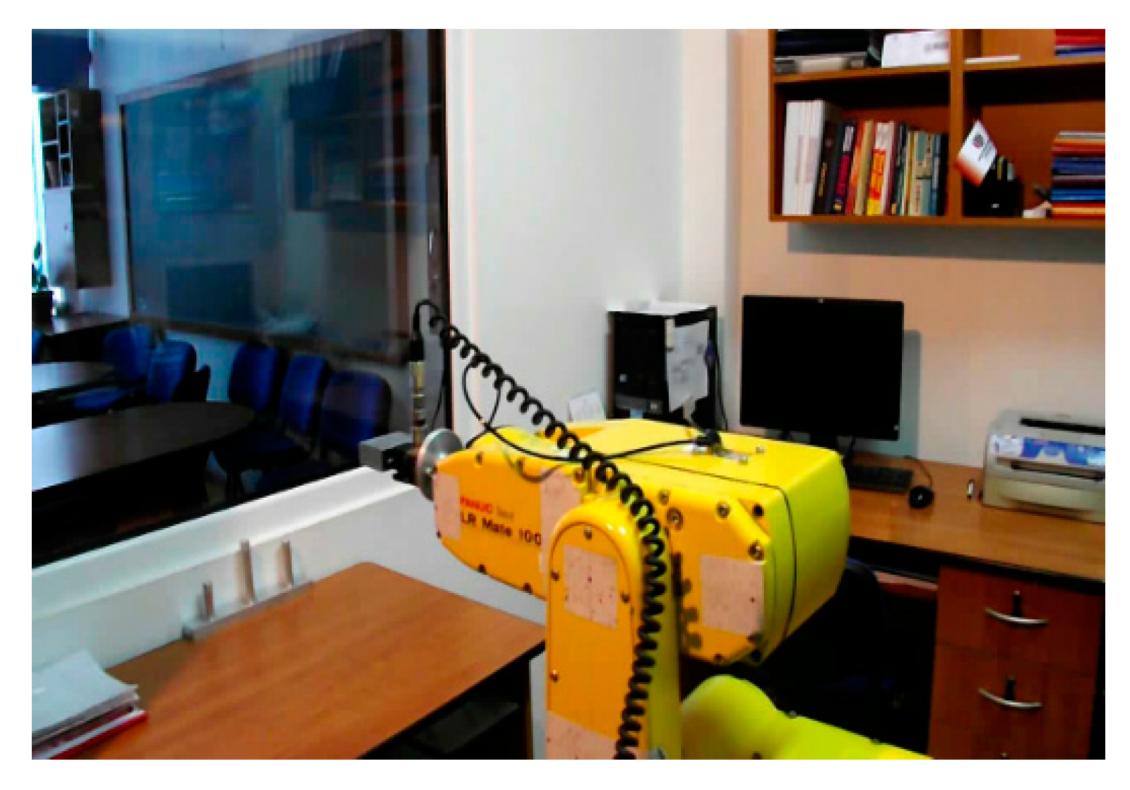
This section was introduced exclusively for highlighting the existence of the accelerations and acceleration energies of the higher order. For this purpose, according to Figure 4, the rotation motion of the arm of the serial robot Fanuc LR Mate 100 iB, on the angular interval was considered. The total time of the rotation motion was of 1.7 s.
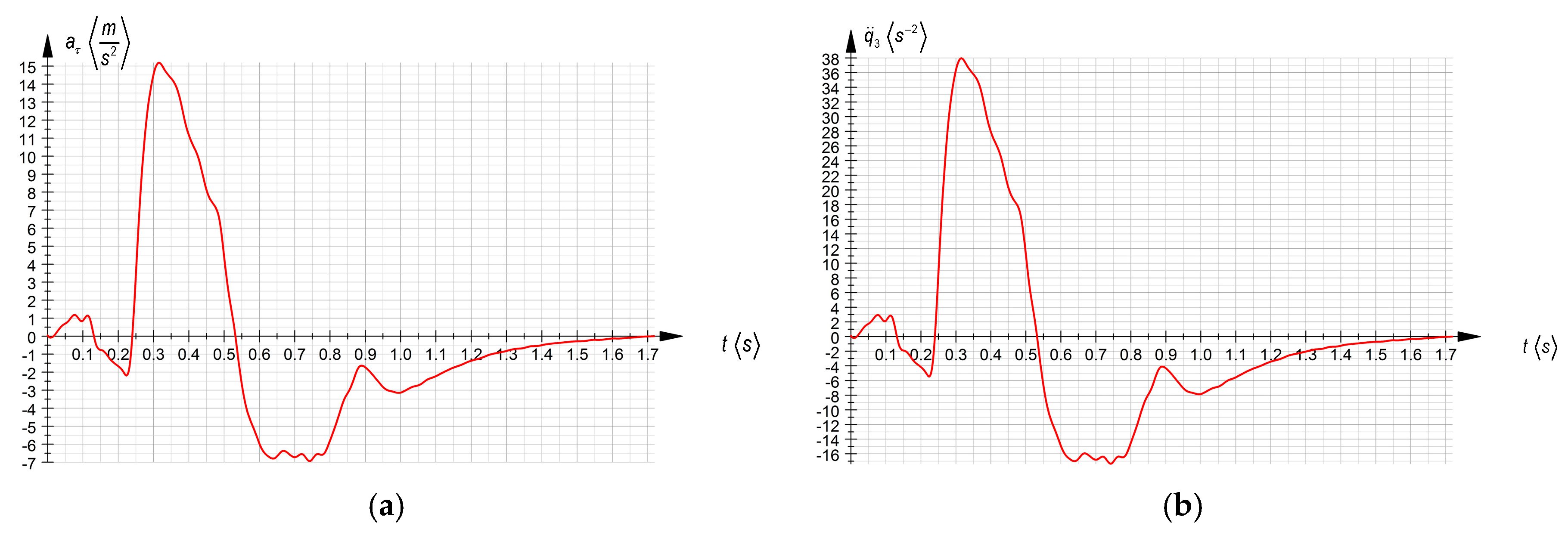
For highlighting the time variation law of the acceleration energies of the higher order, the polynomial interpolating functions of the fifth order have been applied in accordance with (48)–(51). This method requires, according to kinematical constraints (51), the establishment through measurements of the angular acceleration corresponding to robot arm, . As a result, in the first step, the time variation law corresponding to the tangential component of the acceleration for the characteristic point belonging to the robot arm has been determined at every 0.033 s. The experimental data was collected by using a mono-axial accelerometer. The robot arm (more precisely the third kinetic ensemble of the robot) was engaged in rotation motion at high speeds and by using the data collected by the accelerometer. The time variation law for the tangential component of the acceleration of the characteristic point was graphically represented. Considering the rotation motion, in the next step the time variation law of the angular acceleration was also represented. Both graphical representations are illustrated in Figure 5.
According to Figure 5, the maximum value for the linear acceleration exceeds , which defines a sudden motion. The authors have considered, for this application, that the motion can be described by using the polynomial interpolating functions of the fifth order:
where , are the integration constants which are determined from the geometrical and kinematical constraints (50), with an important role in ensuring the continuity of the rotation motion on the angular interval , characterized by 51 interpolation segments. Every interpolation segment contains four unknowns, represented by the integration constants. It is obvious that the total number of the unknowns is 204. In order to determine the unknowns, according to (50), the numerical values for the angular acceleration (Figure 5b) were substituted in the functions (83)–(87) presented above. Considering the large number of results, more exactly 255 polynomial functions, only a few sequences are illustrated in Table 1 and Table 2.
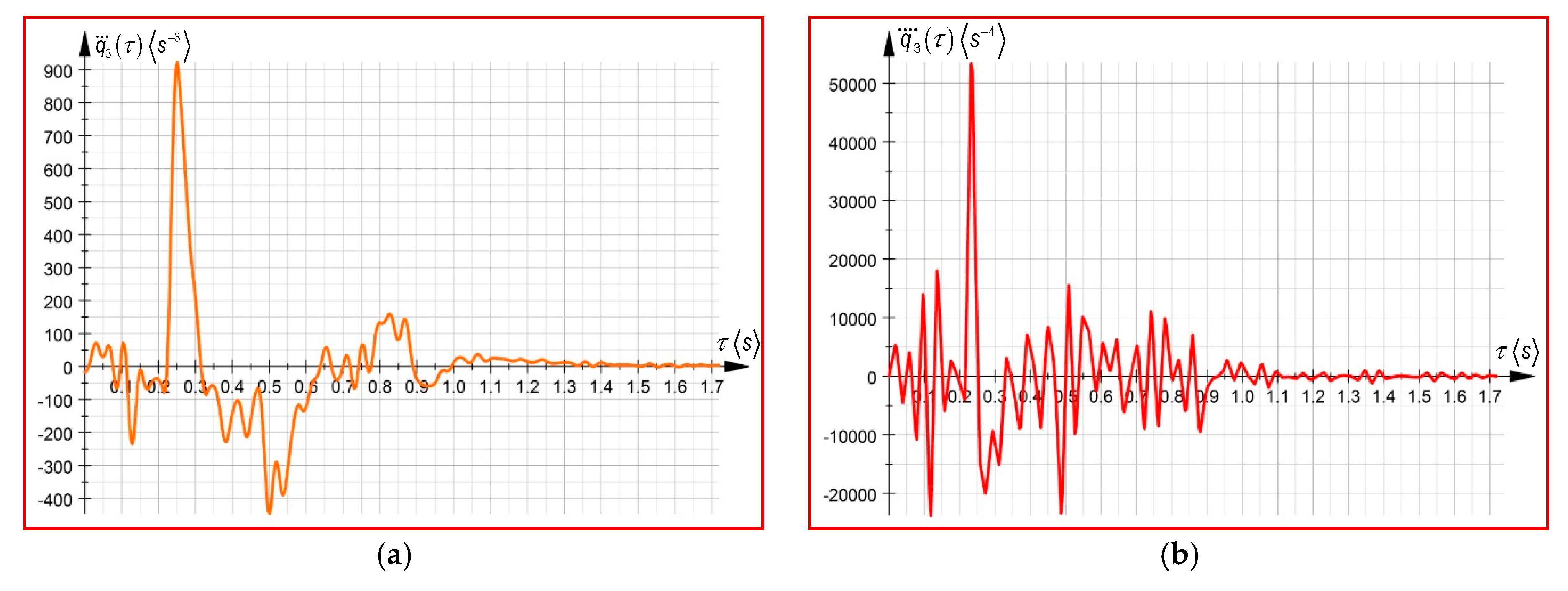
As a result, the numerical values for the angular acceleration (see Figure 5) were applied, finally obtaining all of the integration constants. In order to illustrate this step, some sequences containing the time variation laws of the functions described by Equations (83)–(87) are presented. These results are included in Table 1 and Table 2. Similarly, the polynomial functions are obtained for all the 51 interpolation segments. As a result, the time variation law for the angular acceleration of the second and third order are also graphically represented according to Figure 7:
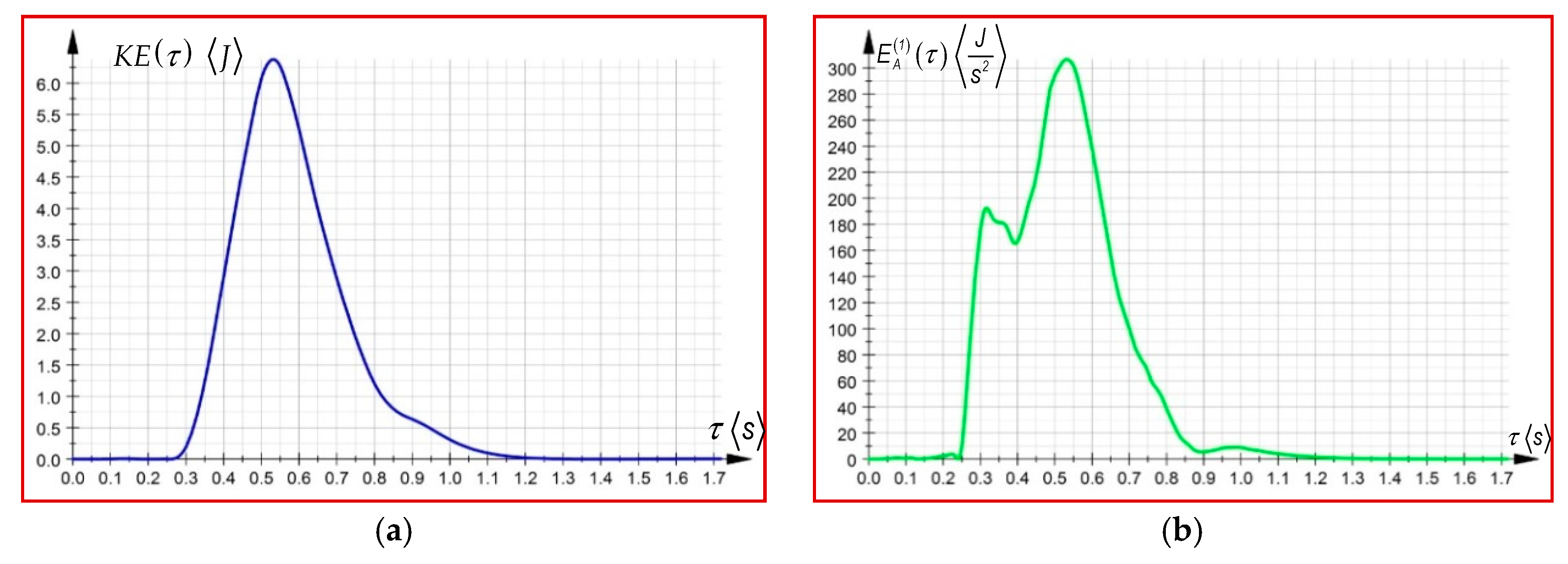
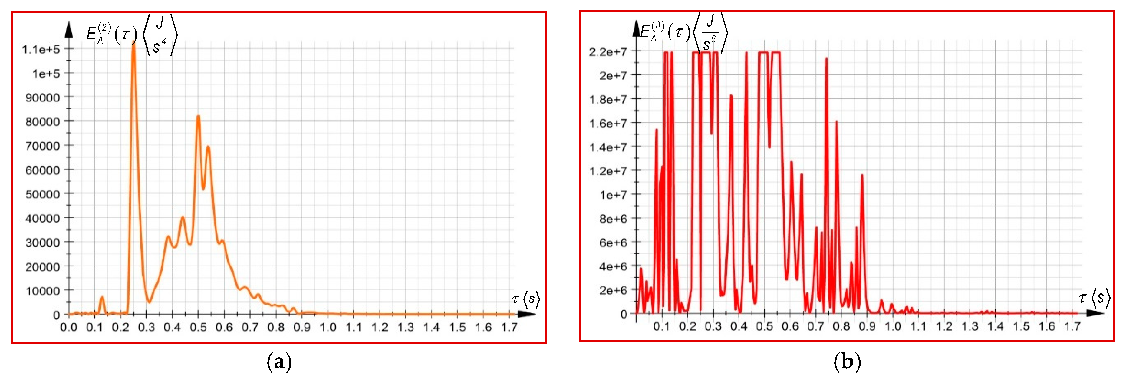
Thus, by customizing Expressions (71), (77)–(80) for the considered robot structure, the following expressions characterizing the acceleration energies of the first, second and third order are:
5. Conclusions
The main objective of this paper was to highlight some new developments in the field of advanced dynamics of mechanical systems and higher order dynamic equations. These equations were developed by using matrix exponentials which proved to have indisputable advantages in the matrix study of any complex mechanical system. In this paper, new approaches have been proposed based on differential principles from analytical mechanics by using some important dynamics notions, regarding the acceleration energies of the first, second and third order. The study was extended to the equations of the higher order, which provided the possibility of applying the initial motion conditions in the positions, velocities and accelerations of the first and second order. In order to determine the time variation laws for the generalized variables and acceleration energies of the higher order, the time polynomial functions of the fifth order were applied. In Newtonian dynamics, the establishment of dynamic equations as second order differential equations are performed by considering the kinetic energy as the main function. In the case of fast and sudden movements, the presence of higher order accelerations leads to higher order differential equations which define the variation laws in relation to time in the case of the forces and the driving moments that impose the motion of the mechanical systems. As a result, the application of acceleration energies highlights, in an explicit and direct form, the presence of higher-order accelerations, unlike the case where the study was performed considering kinetic energy.
In accordance to inverse kinematics, also known as the control kinematics of the robots, the use of polynomial functions leads to the control of the mechanical motion, especially of transitory motions. These aspects were exemplified in the previous section. Therefore, it was noticed that on the time interval of 1.7 s, a number of 51 measurements of the tangential acceleration were performed at every 0.033 s. Regarding the polynomial functions, this aspect led to a very good approximation of the mechanical motion. At the same time, the polynomial functions were substituted in the expressions of the acceleration energies of the higher order. Therefore, their time variation laws were obtained as shown in graphical representations from the previous section.
6. Contributions of the Authors
The purpose of this paper was to present some original defining expressions for acceleration energies of the higher order. These expressions also include the accelerations of the higher order which define the fast and sudden motions of mechanical systems. The novelty of this paper was in determining in an explicit form of the expressions for the acceleration energies based on advanced kinematic notions and using polynomial interpolation functions of the higher order.
Therefore, the contributions of the main author are highlighted by a great number of expressions included in the following sections of this paper:
- 2.1. Position and Orientation Parameters. The new expressions are: (10)–(16), (19) and (20), as well as (24), (27)–(30).
- 2.2. The Kinematic Parameters of Higher Order. The new equations are: (34)–(38) and (42)–(50);
- 3. Higher Order Acceleration Energies. This section contains the new expressions of definition for the acceleration energy of the first, second and third order in an explicit form: (69)–(82).
Author Contributions
Conceptualization, I.N.; methodology, I.N.; investigation and software A.-V.C; validation, I.N.; formal analysis, I.N; resources, I.N., A.-V.C.; data curation, I.N., A.-V.C.; writing—original draft preparation, A.-V.C; writing—review and editing, I.N., A.-V.C.; visualization, A.-V.C; supervision, I.N.
Funding
This research received no external funding.
Acknowledgments
The authors would like to thank Technical University of Cluj Napoca, Romania for providing the technical support in carrying out the experimental analysis.
Conflicts of Interest
The authors declare no conflicts of interest.
References
- Appell, P. Sur Une Forme Générale des Equations de la Dynamique, 1st ed.; Gauthier-Villars: Paris, France, 1899. [Google Scholar]
- Appell, P. Traité de Mécanique Rationnelle, 1st ed.; Garnier frères: Paris, France, 1903. [Google Scholar]
- Craig, J.J. Introduction to Robotics: Mechanics and Control, 3rd ed.; Pearson Prentice Hall: Upper Sadelliffe, NJ, USA, 2005. [Google Scholar]
- Yuan, B.S.; Book, W.J.; Huggins, J.D. Dynamics of Flexible Manipulator Arms: Alternative derivation, Verification, and Characteristics for Control. ASME J. Dyn. Syst. Meas. Control 1993, 115, 394–404. [Google Scholar] [CrossRef]
- Bhatti, M.; Lu, D. Analytical Study of the Head-On Collision Process between Hydroelastic Solitary Waves in the Presence of a Uniform Current. Symmetry 2019, 11, 333. [Google Scholar] [CrossRef]
- Hussain, F.; Ellahi, R.; Zeeshan, A. Mathematical Models of Electro-Magnetohydrodynamic Multiphase Flows Synthesis with Nano-Sized Hafnium Particles. Appl. Sci. 2018, 8, 275. [Google Scholar] [CrossRef]
- Marin, M.; Vlase, S.; Ellahi, R.; Bhatti, M. On the Partition of Energies for the Backward in Time Problem of Thermoelastic Materials with a Dipolar Structure. Symmetry 2019, 11, 863. [Google Scholar] [CrossRef]
- Thompson, P. Snap, Crackle, and Pop, (AIAA Info.); Systems Technology: Hawthorne, CA, USA, 2011. [Google Scholar]
- Eager, D.; Pendrill, A.M.; Reinstad, N. Beyond velocity and acceleration: jerk, snap and higher derivatives. Eur. J. Phys. 2016, 37, 065008. [Google Scholar] [CrossRef]
- Negrean, I.; Negrean, D.C. The Acceleration Energy to Robot Dynamics. In Proceedings of the A&QT-R International Conference on Automation, Quality and Testing, Robotics, Cluj-Napoca, Romania, 23–25 May 2002; pp. 59–64. [Google Scholar]
- Negrean, I.; Negrean, D.C. Matrix Exponentials to Robot Kinematics. In Proceedings of the 17th International Conference on CAD/CAM, Robotics and Factories of the Future, CARS&FOF, Durban, South Africa, 10–12 July 2001; pp. 1250–1257. [Google Scholar]
- Negrean, I. New Formulations on Motion Equations in Analytical Dynamics. Appl. Mech. Mater. 2016, 823, 49–54. [Google Scholar] [CrossRef]
- Negrean, I. Advanced Notions in Analytical Dynamics of Systems. Acta Tech. Napoc. Ser. Appl. Math. Mech. Eng. 2017, 60, 491–502. [Google Scholar]
- Negrean, I. Energies of Acceleration in Advanced Robotics Dynamics. Appl. Mech. Mater. 2014, 762, 67–73. [Google Scholar] [CrossRef]
- Vlase, S.; Teodorescu, P.P. ElastoDynamics of a Solid with A General “Rigid” Motion Using Fem Model Part I. Theoretical Approach. Rom. J. Phys. 2013, 58, 872–881. [Google Scholar]
- Pars, L.A. A Treatise on Analytical Dynamics; Heinemann: London, UK, 2007; Volume 1, pp. 1–122. [Google Scholar]
- Jazar, R.N. Theory of Applied Robotics: Kinematics, Dynamics, and Control, 2nd ed.; Springer Nature Switzerland AG: Basel, Switzerland, 2010. [Google Scholar]
- Ardema, M.D. Analytical Dynamics. Theory and Applications; Springer Nature Switzerland AG: Basel, Switzerland, 2005. [Google Scholar]
- Park, F.C. Computational Aspects of the Product-of-Exponentials Formula for Robot Kinematics. IEEE Trans. Autom. Control 1994, 39, 643–647. [Google Scholar] [CrossRef]
- Brener, P. Technical Concepts. Orientation, Rotation, Velocity and Acceleration, and the SRM. User’s manual, version 2.0; SEDRIS. 2008. [Google Scholar]
Figure 1.
(a) The position and orientation for a point; (b) The position and orientation of a system.
Figure 1.
(a) The position and orientation for a point; (b) The position and orientation of a system.

Figure 2.
The representation of a free rigid body in the Cartesian frame.

Figure 3.
The representation of a kinetical element from robot mechanical structure.

Figure 4.
Fanuc LR Mate 100 iB robot. The location of the transducer on the robot arm.

Figure 5.
(a) Tangential accelerations variation law. (b) Generalized accelerations variation law. The above presented parameters were also determined on the same angular interval , by applying the sudden stop. The graphical representation is illustrated in Figure 6.
Figure 5.
(a) Tangential accelerations variation law. (b) Generalized accelerations variation law. The above presented parameters were also determined on the same angular interval , by applying the sudden stop. The graphical representation is illustrated in Figure 6.

Figure 6.
(a) The tangential first order accelerations variation law; (b) The generalized accelerations of first order variation law.
Figure 6.
(a) The tangential first order accelerations variation law; (b) The generalized accelerations of first order variation law.

Figure 7.
(a) The variation law of the angular accelerations of second order. (b) The variation law for the angular accelerations of third order.
Figure 7.
(a) The variation law of the angular accelerations of second order. (b) The variation law for the angular accelerations of third order.

Figure 8.
(a) The variation law for the kinetic energy. (b) The time variation law of the acceleration energy of the first order.
Figure 8.
(a) The variation law for the kinetic energy. (b) The time variation law of the acceleration energy of the first order.

Figure 9.
(a) The variation law for the acceleration energy of second order; (b) The time variation law of the acceleration energy of third order.
Figure 9.
(a) The variation law for the acceleration energy of second order; (b) The time variation law of the acceleration energy of third order.


Table 1.
The polynomial time functions for the generalized coordinates for the third rotation joint.
Table 1.
The polynomial time functions for the generalized coordinates for the third rotation joint.
| Polynomial Time Functions for Generalized Coordinates | ||
|---|---|---|
Table 2.
The Polynomial Time Functions for Generalized Variables in Case of the Third Rotation Joint.
Table 2.
The Polynomial Time Functions for Generalized Variables in Case of the Third Rotation Joint.
| Polynomial Time Functions for Generalized Variables | |||
|---|---|---|---|
© 2019 by the authors. Licensee MDPI, Basel, Switzerland. This article is an open access article distributed under the terms and conditions of the Creative Commons Attribution (CC BY) license (http://creativecommons.org/licenses/by/4.0/).
Share and Cite
MDPI and ACS Style
Negrean, I.; Crișan, A.-V. Synthesis on the Acceleration Energies in the Advanced Mechanics of the Multibody Systems. Symmetry 2019, 11, 1077. https://0-doi-org.brum.beds.ac.uk/10.3390/sym11091077
AMA Style
Negrean I, Crișan A-V. Synthesis on the Acceleration Energies in the Advanced Mechanics of the Multibody Systems. Symmetry. 2019; 11(9):1077. https://0-doi-org.brum.beds.ac.uk/10.3390/sym11091077
Chicago/Turabian StyleNegrean, Iuliu, and Adina-Veronica Crișan. 2019. "Synthesis on the Acceleration Energies in the Advanced Mechanics of the Multibody Systems" Symmetry 11, no. 9: 1077. https://0-doi-org.brum.beds.ac.uk/10.3390/sym11091077
Note that from the first issue of 2016, this journal uses article numbers instead of page numbers. See further details here.