Kinetic Model for Vehicular Traffic with Continuum Velocity and Mean Field Interactions ^†

Abstract

This paper is concerned with the modeling and mathematical analysis of vehicular traffic phenomena. We adopt a kinetic theory point of view, under which the microscopic state of each vehicle is described by: (i) position, (ii) velocity and also (iii) activity, an additional varible that we use to describe the quality of the driver-vehicle micro-system. We use methods coming from game theory to describe interactions at the microscopic scale, thus constructing new models within the framework of the Kinetic Theory of Active Particles; the resulting models incorporate some of the symmetries that are commonly found in the mathematical models of the kinetic theory of gases. Short-range interactions and mean field interactions are introduced and modeled to depict velocity changes related to passing phenomena. Our main goal is twofold: (i) to use continuum-velocity variables and (ii) to introduce a non-local acceleration term modeling mean field interactions, related to, for example, the presence of tollgates or traffic highlights.

1. Introduction

The mathematical approach to vehicular traffic modeling can be developed at three different observation and representation scales, namely the microscopic, mesoscopic and macroscopic scales. Different mathematical structures correspond to each type of representation:

• microscopic scale: ordinary differential equations for the variable representing the state of each vehicle, viewed as an individual entity;
• mesoscopic scale: integro-differential equations for a probability distribution over the microscopic state of vehicles;
• macroscopic scale: partial differential equations for locally averaged quantities (moments of the aforementioned probability distribution); tipically density, momentum and energy are considered.

Indeed, one of the greatest difficulties of the modeling approach is the adequate choice of the representation scale. The microscopic modeling implies that we have to deal with a large number of equations and the macroscopic choice neglects the role of fluctuations and uncertainties, due the process of averaging. Note also that the last approach considers the vehicle as a single particle, instead of a system embodying both driver and mechanics; the heterogeneous behavior of the driver-vehicle micro system is not taken into account. Accordingly, the critical analysis proposed in the survey paper [1] confronts us with the fact that none of the aforesaid scale approaches is totally satisfactory; a multiscale approach is necessary to obtain a detailed description of the complex dynamics of vehicles on road. Let us comment now on some references in the literature that complement this point of view. In Reference [2] a hybrid model is deduced, where a detailed modeling of the dynamics of the micro-systems is implemented into a macroscopic mass conservation equation. This hybrid model is revisited in Reference [3], with the focus on the implementation of boundary conditions corresponding to the presence of tollgates, junctions or traffic highlights. This is the aim of our work but, in contrast, we will present a mesoscopic kinetic model where the velocity is still an independent variable (as for example in References [4,5,6,7]) related to the state of the driver-vehicle micro-system. We also quote here the survey on the physics and modeling of multi-particle systems [8]. The critical paper by Daganzo [9] points out some drawbacks of the driver-vehicle micro-system, where interactions can even modify the behavior of the driver -whose ability is conditioned by the local flow conditions. Reference [9] has generated various discussions and controversies documented in several works (of which we highlight Reference [10]) and also reactions to account for the aforementioned criticisms [4,5]. The approach of Reference [5] has been further developed by various papers, take for instance the proposal in Reference [6] using a discrete space variable and implementing the model over networks. Further technical developments can be found in Reference [7,11].

Our paper refers to Reference [5], where the authors proposed a kinetic model with the following main features:

• A discrete velocity variable is used.
• The description operates at the mesoscopic scale, in order to account for the heterogeneous behavior of the driver-vehicle micro-system.
• The quality of the road-environment conditions is taken into account by an additional parameter. This parameter takes values between zero and one (zero for worst conditions and one for best conditions respectively) and shall play an explicit role in the description of the interactions.

Our paper is based on the kinetic theory of active particles [12] (KTAP) and draws inspiration from Reference [5]; we mention here the ability of Reference [5] to reproduce: (i) the fundamental diagrams-mean velocity and flow versus local density, (ii) clustering phenomena of vehicles with similar velocity. The analogy with social behavior KTAP models is also worth mentioning here, in particular in the field of opinion formation [13]. Heterogeneity, clustering and interactions described by evolutionary stochastic games are also key points on the modeling paradigm in this area, even if the models do not have space and velocity dependence. We extend Reference [5] by proposing a new, general mathematical structure taking into account all the possible phenomena in vehicular traffic field (short and mean-field interactions, continuous velocity and modulation of the perceived density), thus aiming at providing further developments of interest for the applications. The following modeling topics are considered: (i) interactions between vehicles accounting on perceived quantities of the vehicle flow; (ii) these interactions can be both, local and long-ranged and strongly dependent on the road conditions, (iii) dynamics under external actions (e.g., presence of tollgates). Moreover, rather than discrete velocity variables, we consider a continuous velocity distribution. These new modeling features introduced in this paper constitute what we think is a deep revision of the proposal in Reference [5].

The contents of this paper are the following: we derive a new mathematical structure in Section 2; this structure is suited to include the aforementioned features, together with those already present in Reference [5]; Section 3 shows how to derive specific models by means of inserting into the aforesaid structure various models of interactions; these models are obtained by means of a detailed phenomenological interpretation of the physical reality. Finally, Section 4 provides a brief sketch on how to construct solutions to the models introduced in Section 3.

2. Mathematical Structures

In this section we tackle derivation of a new, general structure, appropriate to include the specific features defined in Section 1. We do this through a sequence of subsections going from the representation of the system to the derivation of the structure. This structure is innovative with respect to the existing literature [5], since it includes modeling local interactions, long-range interactions and interactions with external actions as well. This structure will provide the conceptual basis for the derivation of specific models in Section 3.

2.1. Nondimensional Representation

Let us consider a one-dimensional flow of vehicles along a spatially periodic road of length ℓ; the road is assumed to have a single lane. Position and velocity variables are denoted by x and v. We introduce a limit velocity $v_{\ell }$ such that no vehicle can exceed, simply for mechanical reasons, even in the most favorable environmental conditions. We also introduce $t_c$, the time needed by a vehicle with velocity $v_{\ell }$ to move along the whole road, that is, $t_c:=\ell /v_{\ell }$. This enables us to write down dimensionless position, velocity and time variables by means of

$$\overline{x}:=\frac{x}{\ell },\overline{v}:=\frac{v}{v_{\ell }},\overline{t}:=\frac{t}{t_c}.$$

We shall drop the overlines in what follows.

We will use also dimensionless variables for macroscopic bulk quantities, as for example, the local number density $\rho =\rho (t,x)$ is defined as the actual density over ${\rho }_M$, being the latter the maximum vehicle density which corresponds to bumper-to-bumper traffic jam.

The analysis that we shall carry in this paper is based on the assumption that the state of the driver-vehicle subsystem is specified by the microscopic variables $(x,v,u)\in {[0,1]}^3$. According to the KTAP [12], u is a variable that accounts for the quality of the micro-system. Namely, $u=1$ corresponds to the best quality -think of an experienced driver in a high-quality vehicle, while $u=0$ corresponds to the worst quality, that is, motion is prevented.

Following Reference [12], the subsystem driver-vehicle is regarded as an active particle, the internal variable being heterogeneously distributed over the active particles. We will use a parameter $\alpha \in [0,1]$ to measure the quality of the road including environmental conditions, that may depend on the space variable, that is, $\alpha =\alpha \left(x\right)$, in order to represent curves, local restrictions and so forth. In general, $\alpha =1$ corresponds to the best conditions and $\alpha =0$ corresponds to the worst quality that prevents motion.

We finally describe the overall state of the system by a distribution function over the states at the microscopic scale:

$$f=f(t,x,v,u):{\mathbb{R}}_{+}\times [0,1]\times [0,1]\times [0,1]\to {\mathbb{R}}_{+}.$$

Here as usual we require f to be integrable, so that $f(t,x,v,u)dxdvdu$ denotes the dimensionless distribution of vehicles which at time t have position x, velocity v and activity u. In particular, the local density is given by

$$\rho (t,x)={\int }_0^1{\int }_0^{1}f(t,x,v,u)dvdu.$$

(1)

Recall that $\rho$ is normalized in term of ${\rho }_M$, which imposes a normalization on f.

2.2. Interaction Domains and Perceived Quantities

The active particle (the car-driver subsystem), has a visibility zone ${\Omega }_v={\Omega }_v\left(x\right)=[x,x+{\ell }_v]$, where ${\ell }_v$ is the visibility length on front of the vehicle. As our road is spatially periodic, when $x+{\ell }_v>1$, the visibility zone will be ${\Omega }_v=[0,x+{\ell }_v-1]\cup [x,1]$. This visibility length is assumed to be proportional to the quality of the environment $\alpha$ and much smaller than ℓ. In addition, the active particle has a sensitivity zone, ${\Omega }_{\ell }=[x,x+{\ell }_s]$ (or ${\Omega }_{\ell }=[0,x+{\ell }_s-1]\cup [x,1]$ if $x+{\ell }_s>1$), necessary to perceive the flow conditions in ${\Omega }_{\ell }$. In general ${\Omega }_{\ell }\subseteq {\Omega }_v$. However, we must bear in mind that the opposite case can also take place when the local conditions of the road prevent visibility. The computations in the sequel are developed under the assumption that the visibility zone includes the sensitivity zone. Note also that ${\Omega }_{\ell }$ can, in general, depend on f; this entails an additional nonlinearity.

The driver will develop its driving strategy based on his perception of the state of the other vehicles in ${\Omega }_{\ell }$. Among those vehicles, the ones that are closer to the driver have a stronger influence on his strategy. To account for this, we introduce a (much) smaller domain, say ${\Omega }_s$ within which active particles are assumed to perceive an approximate estimate of the local gradients. Hence (see Reference [4]) active particles perceive a density ${\rho }_p\left[\rho \right]$ which is lower than the real one in the presence of negative gradients and higher than the real one in the presence of positive gradients. We define short-range interactions as those involving vehicles in ${\Omega }_s$ and long-range interactions as those involving vehicles mainly in ${\Omega }_{\ell }\backslash {\Omega }_s$.

In the approach of the KTAP, interactions are modeled after evolutionary stochastic games. We have to consider three different active particle types (driver-vehicle): (i) candidate particles, having the micro-state $\{x,v_{*},u_{*}\}$, (ii) field particles with the state $\{x^{*},v^{*},u^{*}\}$ and (iii) a test particle, which is representative of the whole system. The idea is that candidate particles are localized in x and can interact with field particles (considered to be localized in ${\Omega }_s$ for the case of short-range interactions and in ${\Omega }_{\ell }$ when dealing with long-range—that is, mean field- interactions). As a result of the interaction with the field particle, the candidate particle has a certain probability of acquiring the state of the test particle. The modeling rationale we propose in the following rests on the assumption that interactions does not modify the activity variable of both candidate and test particles.

2.3. Mean Field Interactions

The test vehicle is subject to interactions with those vehicles in its sensitivity zone ${\Omega }_{\ell }$. Both a consensus toward a common velocity (e.g., the mean speed within the visibility domain) and a clustering effect can result form this dynamics. The test vehicle becomes sensitive to these actions whenever the distance between its speed and the common velocity falls below a critical threshold.

Generally speaking, mean field interactions can be described using an individual-based acceleration term $\phi (x,x^{*},v,v^{*},u,u^{*})$. This is applied to the test vehicle $(x,v,u)$ by all the vehicles $(x^{*},v^{*},u^{*})$ in its sensitivity domain ${\Omega }_{\ell }$. Therefore, the overall acceleration is defined as an integral accounting for the action of all vehicles in ${\Omega }_{\ell }$. Thus:

$$\mathcal{F}\left[f\right](t,x,v,u)={\int }_{\Lambda }\phi (x,x^{*},v,v^{*},u,u^{*})f(t,x^{*},v^{*},u^{*})d{x}^{*}d{v}^{*}d{u}^{*},$$

(2)

where $\Lambda :={\Omega }_{\ell }\times [0,1]\times [0,1]$.

2.4. Short-Range Interactions

Short-range interactions involve the smaller domain ${\Omega }_s$, which is enough for a candidate particle to perceive a density ${\rho }_p$. We assume that the distribution of field particles can be approximated by the probability distribution in x. The description of these interactions requires to model two additional quantities:

• The encounter rate$\eta \left[f\right]$, which accounts for the number of interactions per unit time between candidate and test particles with field particles. It depends, a priori, on t and x.
• The transition probability density$\mathcal{A}\left[f\right](v_{*}\to v,v^{*},u)$, which encodes the probability density that a candidate particle with velocity $v_{*}$ falls into the state of the test particle with velocity v after interacting with the field particle with velocity $v^{*}$.

Now, in order to model short-range interactions we shall assume that these quantities depend on the whole distribution function f (and not just on the microscopic state of the interacting particles). This dependence, which is highlighted by the square brackets, induces a nonlinearity at the microscopic scale. These interaction terms may additionally depend on the quality of the road, which is modeled by $\alpha \in [0,1]$. Finally, as a probability density, $\mathcal{A}$ is required to satisfy the condition:

$$\mathcal{A}[f;\alpha ]\ge 0,{\int }_{[0,1]}\mathcal{A}[f;\alpha ](v_{*}\to v,v^{*},u)dv=1,$$

(3)

for all possible inputs $v_{*}$, $v^{*}$, u. Note that this kernel needs not be a probability density with respect to the x or u variables and then some integrability hypothesis should be accordingly added. Instead, we will propose an explicit expression for this term in Section 3.4; under that definition, the kernel will be a bounded function.

2.5. Interactions with External Actions

External actions may influence the test vehicle speed as well. Think for instance about tollgates; these enforce a maximal speed for approaching vehicles. Also, the way in which the speed can increase to the standard values after exiting the tollgate is also indicated. The effects caused by speed limits can be also described as an external action.

We model this term in the simplest way, by in using a relaxation-type term:

$$\mathcal{T}\left[f\right](t,x,v,u)=\mu [f,x]\left(f_e(x,v_e\left(x\right))-f(t,x,v,u)\right),$$

(4)

where $\mu [f,x]$ represents the intensity of the action, which increases with $\rho$, while the given external density $f_e(x,v_e\left(x\right))$ is suppose to adapt the velocity of the vehicles to $v_e\left(x\right)$. Note that $\mu$ vanishes at those regions where external actions play no role.

2.6. Assembling a Mathematical Structure

This subsection shows how all action models that were described above can be integrated within a proper mathematical structure; this structure shall offer the conceptual basis for the derivation of different models. The structure results from a particle balance within a elementary volume in the space of microscopic states. This volume includes the phase space variables (position and velocity) together with the activity variable. The particle balance accounts for the free transport term, the transitions due to long-range interactions, the dynamics of short-range, conservative interactions (consisting in a “gain” and a “loss” term) and the trend to the velocity enforced by the external actions. At a formal level, we can write the resulting structure as follows:

$${\partial }_{t}f+v{\partial }_{x}f+F\left[f\right]=J\left[f\right]+\mathcal{T}\left[f\right].$$

Here F, J and $\mathcal{T}$ account for mean field interactions, short-range interactions and interactions with external actions respectively. More concretely, the structure can be written as

$$\begin{array}{cc}\hfill & {\partial }_{t}f(t,x,v,u)+v{\partial }_{x}f(t,x,v,u)+{\partial }_v\left(\mathcal{F}\left[f\right](t,x,v,u)f(t,x,v,u)\right)\hfill \\ =& {\int }_{{[0,1]}^3}\eta \left[f\right]\mathcal{A}[f;\alpha ](v_{*}\to v,v^{*},u)f(t,x,v_{*},u)f(t,x,v^{*},u^{*})d{v}_{*}d{v}^{*}d{u}^{*}\hfill \\ & -f(t,x,v,u){\int }_{{[0,1]}^2}\eta \left[f\right]f(t,x,v^{*},u^{*})d{v}^{*}d{u}^{*}+\mu [f,x]\left(f_e(x,v_e\left(x\right))-f(t,x,v,u)\right).\hfill \end{array}$$

(5)

It is worth mentioning that the nonlinear operator $J\left[f\right]$, which is also local with respect to x, resembles the collision kernel of Boltzmann’s equation in the kinetic theory of gases; besides, the kernel $\mathcal{A}$ depends on f, which gives us an idea of the complexity of the mathematical structure of our approach.

2.7. Critical Analysis

In the authors’ opinion, the following aspects of the dynamics should be taken into account when developing traffic models: the heterogeneity of the driver-vehicle subsystem, passing probabilities, aggregation dynamics for vehicles with similar velocities, the role of external actions and also the variable properties of the road-environment where the dynamics occur. We propose here a mathematical structure that is capable of including the above list of features.

The aforesaid structure can operate as a general model derivation framework; interaction rules at the microscopic scale are fed to the global structure to obtain various models. One way to do this is by means of a phenomenological interpretation of empirical data, we quote here the book by Kerner [14] in that regard (empirical data valid in both uniform flow conditions and in transient conditions are provided; see also Reference [15]). However, we note that individual behaviors in unsteady conditions are quite different from those in steady conditions. Nevertheless, we hope that a sharp interpretation of available data will lead to models able to be validated with the information coming from new empirical data.

3. Going from Mathematical Structures to Specific Models

Here we develop an approach to the derivation of specific models of vehicular traffic. The procedure we outline below consists on inserting into the structure (5) models of interactions at microscopic scale. We seek a good agreement with empirical data (specifically the fundamental diagram and the emerging behaviors in unsteady flow conditions) and this will guide our descriptions of the interaction terms $\phi$, $\eta$, $\mathcal{A}$, $\mu$ and $f_e$ characterizing the aforementioned structure.

3.1. Modeling Accelerations

The acceleration term $\phi$ introduced in (2) accounts for mean field interactions. Recall that the test vehicle is subject to the action of those vehicles in front of it and within its sensitivity zone ${\Omega }_{\ell }$; this can induce a consensus toward a common velocity. We pose the following phenomenological interpretation of reality: the test vehicle is sensitive to these actions provided that the distance between its velocity v and the observed velocity $v^{*}$ is below a certain critical threshold $d_c$; actually, its acceleration decays with the distance between the test and field vehicle, taking the sign of $v^{*}-v$ and being proportional to the quality of both the driver-vehicle and the road, through u and $\alpha$. Then, we propose the following acceleration term:

$$\phi (x,x^{*},v,v^{*},u):=\left\{\begin{array}{ccc}{\displaystyle \alpha u\frac{x^{*}-x}{{\ell }_v}(v^{*}-v)}\hfill & if& |v^{*}-v|\le d_c,\hfill \\ 0\hfill & if& |v^{*}-v|>d_c.\hfill \end{array}\right.$$

(6)

Note that our definition of $\phi$ does not depend on $u^{*}$. Whenever $x^{*}\in {\Omega }_{\ell }=[x,x+{\ell }_v]$ we have $0\le \frac{x^{*}-x}{{\ell }_v}\le 1$ and taking $z^{*}=\frac{x^{*}-x}{{\ell }_v}$ in (2), it becomes

$$\begin{array}{ccc}\hfill \mathcal{F}\left[f\right]& =& {\ell }_v{\int }_{{[0,1]}^3}\phi (x,x+{\ell }_v{z}^{*},v,v^{*},u)f(t,x+{\ell }_v{z}^{*},v^{*},u^{*})d{z}^{*}d{v}^{*}d{u}^{*}\hfill \\ & =& \alpha u{\ell }_v\left({\mathcal{F}}_1\left[f\right](t,x)-v{\mathcal{F}}_2\left[f\right](t,x)\right),\hfill \end{array}$$

(7)

where

$$\begin{array}{ccc}\hfill {\mathcal{F}}_1\left[f\right](t,x)& =& {\int }_0^1{\int }_{B^{*}}{\int }_0^1{z}^{*}{v}^{*}f(t,{\ell }_v{z}^{*}+x,v^{*},u^{*})d{z}^{*}d{v}^{*}d{u}^{*},\hfill \\ \hfill {\mathcal{F}}_2\left[f\right](t,x)& =& {\int }_0^1{\int }_{B^{*}}{\int }_0^1{z}^{*}f(t,{\ell }_v{z}^{*}+x,v^{*},u^{*})d{z}^{*}d{v}^{*}d{u}^{*},\hfill \end{array}$$

with $B^{*}=\{v^{*}\in [0,1]:|v^{*}-v|<d_c\}$. In particular, the derivative of $\mathcal{F}$ with respect to v yields

$${\partial }_v\left(\mathcal{F}\left[f\right]\right)(t,x,v,u)=-\alpha u{\ell }_v{\mathcal{F}}_2\left[f\right](t,x).$$

(8)

3.2. Modeling the Perceived Density

The concept of perceived density was introduced in Reference [16]. Following Reference [16], this quantity should be smaller (greater) than the real one in the presence of negative (positive) density gradients. For that aim, the following expression was introduced in Reference [4]:

$${\rho }_p\left[\rho \right]\equiv {\rho }_p\left[\rho (t,x)\right]:=\rho +\frac{{\partial }_x\rho }{\sqrt{1+{\left({\partial }_x\rho \right)}^2}}\left[(1-\rho )H\left({\partial }_x\rho \right)+\rho H(-{\partial }_x\rho )\right],$$

(9)

where $H(·)$ is the Heaviside function. Thus, the perceived density increases the value of $\rho$ to the largest admissible value $\rho =1$ in the presence of positive gradients, while in the presence of negative gradients the perceived density decreases from the actual density $\rho$ to the lowest admissible value $\rho =0$.

In our framework, which includes mean field interactions through a force term, this type of models for the perceived density can lead to incorrect results. More concretely, in previous models with discrete velocity and no acceleration, the density $\rho$ and the perceived density ${\rho }_p$ remain between zero and one (in a nondimensional representation) and this fact is essential to define the transition probability densities that are involved in the other terms. However, in our new framework with continuous velocity variable we cannot ensure a priori that the density $\rho$ will remain below one for all time; this is due to the presence of the new acceleration term.

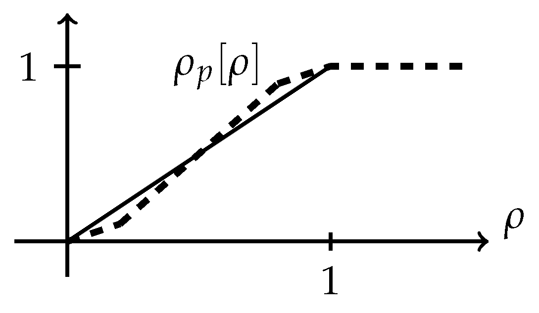
Here we present a simplified scenario in which the above issue is fixed, keeping the spirit of formula (9) as much as possible. For that aim we introduce a controlled perceived density—which, by the way, does not involve gradients, thus producing a simpler mathematical model. If we assume that the influence of positive gradients is most relevant when: (i) the actual density is high, which tends to increase the value of the perceived density, (ii) the actual density is low, which tends to decrease the value of the perceived density, then we can propose a piecewise linear version of (9), see Figure 1 below. Actually, we propose a perceived density ${\rho }_p\left[\rho \right]$ as a Lipschitz function of $\rho$ (dashed line on the picture) which represents the effect of negative gradients for $\rho \sim 0$, the effect of positive gradients for $\rho \sim 1$ and enforces the maximum perceived density to lie between zero and one. The last property will be essential in what follows to construct the transition probability densities modeling short-range interactions.

3.3. Modeling the Encounter Rate

The encounter rate $\eta \left[f\right]$ introduced in Section 2.4 describes the rate of interactions between candidate and test particles with field particles. We assume that this term increases when the local perceived density increases, starting from a minimal value ${\eta }_0$-corresponding to driving in vacuum conditions. We propose the following expression:

$$\eta \left[f\right](t,x)={\eta }_0(1+{\gamma }_{\eta }{\rho }_p\left[\rho (t,x)\right]),$$

(10)

where ${\gamma }_{\eta }$ is the growth coefficient and ${\rho }_p$ is the perceived density defined in the previous paragraph.

3.4. Modeling Short-Range Interactions

Let us introduce the transition probability density $\mathcal{A}\left[f\right](v_{*}\to v,v^{*},u)$ modeling short-range interactions. As said before, this term accounts for the probability density for a candidate particle having the state $\{x,v_{*},u\}$ to acquire the state $\{x,v,u\}$ (state of the test particle) after interaction with the field particles with state $\{x,v^{*},u^{*}\}$. Note that the activity variable is not modified by the interaction (which, however, modifies the speed) as hinted by the notation.

The modeling approach proposed in our paper is based on the following assumptions, which actually represent, from a continuous point of view, the velocity-discrete table of games introduced in Reference [5]:

• Short-range interactions just modify the velocity -they do not modify the activity variable.
• A priori, $\mathcal{A}$ should depend on the following: (i) the velocities of the interacting particles, (ii) the perceived density, (iii) the activity variable and (iv) the quality of the road. In this way, we have $\mathcal{A}=\mathcal{A}(v_{*}\to v,v^{*},u,\alpha ,{\rho }_p)$. Here the dynamics is enhanced by the product $\alpha u$ and limited by the perceived density -actually, it is totally prevented whenever ${\rho }_p=1$.
• We assume that the candidate particle with velocity $v_{*}$, after interacting with the field particles with velocity $v^{*}$, reaches a new velocity v that belongs to the interval $[v_m,v_M]$ given by

  $$v_m=max\{0,min\{v_{*},v^{*}\}-\kappa (1-\alpha u){\rho }_p\left(\right|v_{*}-v^{*}|+exp(-|v_{*}-v^{*}\left|\right)\left)\right\},$$

  (11)

  $$v_M=min\{1,max\{v_{*},v^{*}\}+\kappa \alpha u(1-{\rho }_p)\left(\right|v_{*}-v^{*}|+exp(-|v_{*}-v^{*}\left|\right)\left)\right\}.$$

  (12)
  In the above $\kappa$ is a small constant; this enables $v_m$ to be close to the $min\{v_{*},v^{*}\}$ and $v_M$ to be close to the $max\{v_{*},v^{*}\}$. Note that these choices of $v_m$ and $v_M$ guarantee the fulfillment of the condition $0<v_m<v_M<1$ even if $v_{*}=v^{*}$.

To proceed, we must consider the following two scenarios separately:

3.4.1. Interaction with Faster Particles

If $v_{*}\le v^{*}$, that is, if the candidate particle detects faster field particles, it has a trend to maintain its velocity or to increase it and, in the latter case, the probability of accelerating decreases with $v-v_m$ where $v\in [v_m,v_M]$. We propose the following probability density,

$$\mathcal{A}\left[f\right](v_{*}\to v,v^{*},u)=(1-\alpha u(1-{\rho }_p))\frac{e^{-\frac{|v-v_{*}{|}^2}{{\sigma }_1}}}{Z\left({\sigma }_1\right)}+\alpha u(1-{\rho }_p)\frac{{(v_M-v)}^2}{Z_2},v\in [v_m,v_M],$$

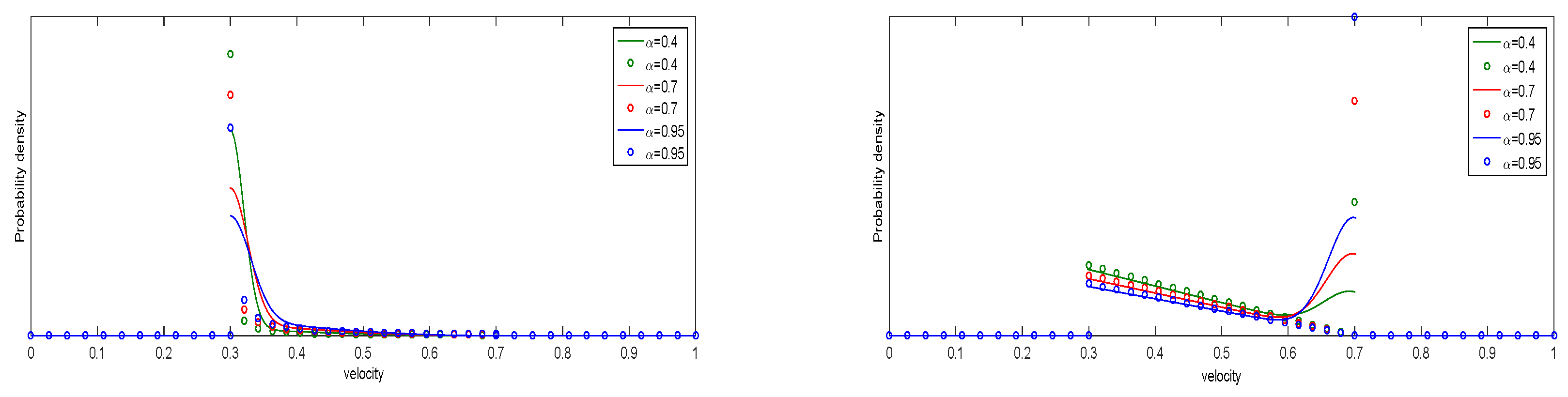
and zero otherwise. This generalizes the table of games defined in Reference [5] in the case of discrete velocities. Here the variance ${\sigma }_1$ represents a tendency of the particle to modify its velocity under good conditions and it is given by ${\sigma }_1=\kappa \alpha u(1-{\rho }_p)$ with $\kappa \ll 1$. Moreover, $Z\left(\sigma \right)={\int }_{v_m}^{v_M}{e}^{-\frac{|v-v_{*}{|}^2}{\sigma }}dv$ and $Z_p={\int }_{v_m}^{v_M}{(v_M-v)}^{p}dv$ are the respective partition functions, which enforce the normalization condition ${\int }_0^1\mathcal{A}dv=1$. We note (see Figure 2 (left)) that this probability density has analogous nonlinear behavior as that of the table of games in Reference [5]. More precisely, in good road conditions $\alpha$ and activity u, the candidate particle has a tendency to accelerate, thus reaching new velocities greater than its pre-interaction velocity $v_{*}$. Quite the contrary, decreasing the value of $\alpha$ or u diminishes the probability of accelerating.

3.4.2. Interaction with Slower Particles

When $v_{*}>v^{*}$, that is, if the candidate particle detects slower field particles, it has a tendency to decrease its velocity or to maintain it. In order to reproduce the behavior of the discrete table of games by Reference [5], we propose the following dichotomy function as the corresponding probability density ruling these interactions:

$$\mathcal{A}\left[f\right](v_{*}\to v,v^{*},u)=\alpha u(1-{\rho }_p)\frac{e^{-\frac{|v-v_{*}{|}^2}{{\sigma }_2}}}{Z\left({\sigma }_2\right)}+(1-\alpha u(1-{\rho }_p))\frac{v_M-v}{Z_1},v\in [v_m,v_M].$$

Note that $\mathcal{A}\left[f\right]$ is set to zero for $v\notin [v_m,v_M]$. Here we have ${\sigma }_2=\kappa (1-\alpha u(1-{\rho }_p))$; the partition functions are defined as in the previous paragraph. We remark that if $\alpha \to 0$ or $u\to 0$, the probability to decelerate is greater than the probability of keeping the current velocity. On the contrary, if $\alpha \to 1$ and $u\to 1$, the candidate particle has a tendency to maintain its velocity (see Figure 2 (right)).

Now the global transition probability density $\mathcal{A}\left[f\right]=\mathcal{A}\left[f\right](v_{*}\to v,v^{*},u)$ can be rewritten accordingly:

$$\begin{array}{ccc}\hfill \mathcal{A}\left[f\right](v_{*}\to v,v^{*},u)& =& [H(v^{*}-v_{*})\left((1-P)\frac{e^{-\frac{|v-v_{*}{|}^2}{{\sigma }_1}}}{Z\left({\sigma }_1\right)}+P\frac{{(v_M-v)}^2}{Z_2}\right)\hfill \\ \hfill & \hfill & +(1-H(v^{*}-v_{*}))\left(P\frac{e^{-\frac{|v-v_{*}{|}^2}{{\sigma }_2}}}{Z\left({\sigma }_2\right)}+(1-P)\frac{v_M-v}{Z_1}\right)]{\chi }_{[v_m,v_M]}\left(v\right).\hfill \end{array}$$

(13)

We use the shorthand notation $P=\alpha u(1-{\rho }_p)$, being $H(·)$ the Heaviside function and ${\chi }_B$ the characteristic function of a set B.

3.5. Modeling External Actions

The effect of external actions is to enforce a prescribed speed, as it occurs , for example, in the presence of tollgates. This term is described as in Equation (4), where $f_e$ is a given function of the prescribed velocity $v_e=v_e\left(x\right)$ -a step-wise function, say. Therefore, the simplicity of Equation (4) entails that only the rate $\mu$ needs to be modeled. Following the same rationale applied to the encounter rate $\eta$ in Section 3.3, the following expression can be used:

$$\mu \left[f\right](t,x)={\mu }_0\left(x\right)(1+{\gamma }_{\mu }{\rho }_p\left[\rho (t,x)\right]),$$

(14)

where ${\gamma }_{\mu }$ is the growth coefficient and ${\rho }_p$ is the perceived density, whereas ${\mu }_0$ accounts for the spatial localization of the external actions.

3.6. Parameters and Final Model

The interaction terms to be implemented into the structure provided by Equation (5) have been modeled in a simple way along this section. The resulting model includes the following parameters, relating to diverse aspects of vehicular traffic flows:

• $\alpha$ quantifies the quality of the road-weather conditions;
• ${\ell }_v$ is the length of the sensitivity zone ${\Omega }_{\ell }$. It depends on $\alpha$ by means of ${\ell }_v=\alpha L$;
• ${\eta }_0$ is the minimal value of the encounter rate;
• ${\gamma }_{\eta }$ and ${\gamma }_{\mu }$ which stand for the growth coefficient of the encounter rate $\eta$ and the intensity of the action $\mu$, respectively.

Bearing in mind the proposed modeling of the interaction terms, we get our definitive traffic model:

$$\begin{array}{cc}\hfill & {\partial }_{t}f(t,x,v,u)+v{\partial }_{x}f(t,x,v,u)+{\partial }_v\left(\mathcal{F}\left[f\right](t,x,v,u)f(t,x,v,u)\right)\hfill \\ =& {\int }_{{[0,1]}^3}\eta \left[f\right]\mathcal{A}\left[f\right](v_{*}\to v)f(t,x,v_{*},u)f(t,x,v^{*},u^{*})d{v}_{*}d{v}^{*}d{u}^{*}\hfill \\ & -f(t,x,v,u){\int }_{{[0,1]}^2}\eta \left[f\right]f(t,x,v^{*},u^{*})d{v}^{*}d{u}^{*}+\mu [f,x]\left(f_e(x,v_e\left(x\right))-f(t,x,v,u)\right).\hfill \end{array}$$

(15)

It is worth mentioning that in this paper we have proposed a probability density (13) by drawing inspiration on the table of games proposed by Reference [5], that features discrete velocity and activity variables. Moreover, we included mean field interactions and nonlinear interactions as well (taking into account the perceived density ${\rho }_p$), considered as one of the paradigms of complexity. A few works proposing to model the probability density in terms of a continuous velocity variable can be found in the vehicular traffic literature, see for example, References [7,17].

4. An Iterative Method to Construct Solutions

In this section we propose a scheme to construct a solution of (15) by means of an iterative method. We shall pose the (linear) approximating problems on the whole space $[0,\infty ]\times {\mathbb{R}}^3$ in order to rely on well-known results for linear transport equations and then we will prove that this amounts to a periodic extension of the linearization of the original problem. Note that accelerations could produce, a priori, velocities out of the interval $[0,1]$, which also justifies the extension to the whole $\mathbb{R}$. With the aid of this extension we will prove in Lemma 1 below that this possibility does not actually take place. Thus, we will first consider a linearized version of model (15) on $[0,\infty ]\times {\mathbb{R}}^3$ and state some properties that will enable us to construct approximate solutions.

4.1. Linearized Transport Model

As our starting point we consider the following transport model on $(t,x,v,u)\in [0,\infty ]\times {\mathbb{R}}^3$:

$${\partial }_{t}f+v{\partial }_{x}f+{\partial }_v\left(\mathcal{F}\left[h\right]f\right)=g,f(0,x,v,u)=f_0(x,v,u).$$

(16)

Here h and g are given; these are smooth functions on $[0,\infty ]\times {\mathbb{R}}^3$. We assume those to be 1-periodic on x and also to vanish for $(v,u)\notin {[0,1]}^2$. The initial data $f_0$ is assumed to be smooth, 1-periodic on x and compactly supported on $(v,u)\in {[0,1]}^2$. The acceleration term $\mathcal{F}\left[h\right]$ is given by (7) for $(t,x,v,u)\in [0,\infty ]\times {\mathbb{R}}^3$ and in this fashion it is 1-periodic in x. Note that our original model (15) is posed on $(t,x,v,u)\in [0,\infty ]\times {[0,1]}^3$; we start by proving that, under natural hypothesis, solutions of (16) preserve the periodicity property on x and the support property for v and u.

Lemma 1

(Periodicity and support). Let h, g and $f_0$ be smooth functions, vanishing for $(v,u)\notin {[0,1]}^2$ and 1-periodic in x. Then, the function f verifying (16) does also vanish for $(v,u)\notin {[0,1]}^2$ and is 1-periodic in x, for all $t\ge 0$.

Proof. 

Thanks to well-known results (see References [18,19] for example), a regular solution of (16) exists, is unique and can be represented explicitly in terms of its characteristic curves, as we will see straightaway on formula (19). Denote these curves by $\left(X\right(s),V(s),U(s\left)\right)$, they depend on an initial tuple $(t,x,v,u)$ and are determined as the solutions to

$$\begin{array}{c}{X}^{\prime }\left(s\right)=V\left(s\right),V^{\prime }\left(s\right)=\mathcal{F}\left[h\right](s,X\left(s\right),V\left(s\right),U\left(s\right)),U^{\prime }\left(s\right)=0,0\le s\le t,\hfill \\ X\left(t\right)=x,V\left(t\right)=v,U\left(t\right)=u.\hfill \end{array}$$

(17)

We will also use the notation $\left(X\right(s,x),V(s,v),U(s,u\left)\right)$ whenever we need to stress the dependence on initial conditions. We remark that under our assumptions the transport field can be easily shown to be locally Lipschitz; this ensures that the associated charateristic curves given by (17) are well-defined objects in the classical sense.

Let us show that the following equality

$$\left(X(s;x)+k,V\left(s\right),u\right)=\left(X(s;x+k),V\left(s\right),u\right),\forall k\in \mathbb{N},$$

(18)

holds. Actually, we only have to observe that the acceleration term $\mathcal{F}\left[h\right]$ is 1-periodic with respect to x provided h is. Then we note that the initial value problems verified by both sides of equality (18) are the same. The uniquenes of this initial value problem concludes the proof of (18). Note in passing that, denoting by $J(s,t)$ the Jacobian of the change $(x,v,u)\mapsto \left(X\right(s),V(s),U(s\left)\right)$ (which depends implicitly on x), we can deduce the same periodicity property (18) for $J(s,t)$; for that we just take derivatives on (18) to obtain the jacobian and use the smoothness of h.

Next we prove the following: if $V\left(t\right)=v\notin [0,1]$ then the V-component of the solution of (17) verifies that $V\left(s\right)\notin [0,1]$. It is equivalent to show the same property for the solution of the “forward” Cauchy problem (17), that is, we take $t=0$ and $s\ge 0$ and we show that $V(s;v)\in [0,1]$ when $V\left(0\right)=v\in [0,1]$, for all $s\ge 0$. We argue by contradiction. Recall that

$$\mathcal{F}\left[h\right]=\alpha u{\ell }_v\left({\mathcal{F}}_1\left[h\right](t,x)-v{\mathcal{F}}_2\left[h\right](t,x)\right)$$

and note that ${\mathcal{F}}_2\left[h\right]\ge {\mathcal{F}}_1\left[h\right]$. Assume that, for some positive time $s>0$, we have $V(s;v)>1$ and then define $s_1=inf\{s\ge 0:V(s;v)>1\}$. Thus, $V(s_1;v)=1$ and there exists some $ϵ>0$ such that $V(s_1+ϵ;v)>1$ and $V^{\prime }(s_1+ϵ;v)>0$. We arrive to a contradiction because

$$\begin{array}{ccc}\hfill 0& <& V^{\prime }(s_1+ϵ;v)=\alpha u{\ell }_v\left({\mathcal{F}}_1\left[h\right](t,X\left(s\right))-V(s_1+ϵ;v){\mathcal{F}}_2\left[h\right](t,X\left(s\right))\right)\hfill \\ & \le & \alpha u{\ell }_v\left({\mathcal{F}}_1\left[h\right](t,X\left(s\right))-{\mathcal{F}}_2\left[h\right](t,X\left(s\right))\right)\le 0.\hfill \end{array}$$

Analogously, arguing by contradiction we can prove that, for any positive time $s>0$, we have $V(s;v)\ge 0$, which concludes the argument. To prove the analogous property with respect to the variable u is straightforward, given that $U\left(s\right)=u$ for all s.

Finally, we conclude the proof of Lemma 1 by writting the solution of (16) as

$$f(t,x,v,u)=J(0,t)f_0(X\left(0\right),V\left(0\right),u)+{\int }_0^{t}J(s,t)g(s,X\left(s\right),V\left(s\right),u)ds,$$

(19)

and using the properties of X, V and U we just proved above. □

Next lemma, where ${\parallel ·\parallel }_{L^p}$ stands for the norm on $L^p\left({[0,1]}^3\right)$, shows us some a priori estimates about the solutions, which can be found in References [18,19]; for the sake of completeness, we present here a sketch of the proof.

Lemma 2

(L^p estimates). Given h, g and $f_0$ verifying the hypothesis of Lemma 1 and such that

$$\parallel f_0{\parallel }_{L^p}+{\parallel h(t,·)\parallel }_{L^p}+{\parallel g(t,·)\parallel }_{L^p}<C<\infty$$

for all $t\ge 0$ and $p=1,\infty$, then, (16) has a unique solution given by (19) and verifying

$${\parallel f(t,·)\parallel }_{L^p}<C\left(T\right)<\infty ,$$

for any $T>0$ and $t\in [0,T]$.

Proof. 

The theory of linear transport equations shows that the Jacobian satisfies ${\partial }_{s}J(s,t)=J(s,t){\partial }_v\left(\mathcal{F}\left[h\right]\right)(s,X\left(s\right),V\left(s\right),u)$ and $J(t,t)=1$. Then, using (8), the equation for J reads ${\partial }_{s}J(s,t)=-\alpha J(s,t)u{\ell }_v{\mathcal{F}}_2\left[h\right](s,X\left(s\right))$. Upon integration,

$$J(s,t)=exp\left\{-{\int }_t^s\alpha u{\ell }_v{\mathcal{F}}_2\left[h\right](\tau ,X\left(\tau \right))d\tau \right\}.$$

We remark that J is not compactly supported in $(v,u)$; However, all the instances of J in (19) are multiplied by functions that are compactly supported in $(v,u)$. Then, taking $L^p$ norms on (19) we obtain the desired estimate with

$$C\left(T\right)=e^{{T\parallel h\parallel }_{\infty }}\parallel f_0{\parallel }_p+T{e}^{{T\parallel h\parallel }_{\infty }}{\parallel g\parallel }_p.$$

When $p=1$ this can be refined to $C\left(T\right)=\parallel f_0{\parallel }_1+{\int }_0^t{\parallel g\left(s\right)\parallel }_{1}ds.$ □

4.2. The Iterative Procedure for the Full Traffic Model

Let us now address the full model (15), posed on the whole space $[0,\infty ]\times {\mathbb{R}}^3$ and with a perceived density ${\rho }_p$ given by the Lipschitz function introduced on on Section 3.2. In order to do that, let us consider, for $n\in \mathbb{N}$, the following iterative scheme:

$${\partial }_t{f}^{n+1}+v{\partial }_x{f}^{n+1}+{\partial }_v\left(\mathcal{F}\left[f^n\right]f^{n+1}\right)=g^n,for(t,x,v,u)\in [0,\infty ]\times {\mathbb{R}}^3.$$

(20)

This is the linear transport Equation (16) with $h=h^n=f^n$, where $g=g^n$ is given by:

$$\begin{array}{ccc}\hfill g^n(t,x,v,u)& :=& {\int }_{{[0,1]}^3}\eta \left[f^n\right]\mathcal{A}\left[f^n\right](v_{*}\to v)f^n(t,x,v_{*},u)f^n(t,x,v^{*},u^{*})d{v}_{*}d{v}^{*}d{u}^{*}\hfill \\ & & -f^n{\int }_{{[0,1]}^2}\eta \left[f^n\right]f^n(t,x,v^{*},u^{*})d{v}^{*}d{u}^{*}+{\mu }_n[f^n,x]\left(f_e^n(x,v_e\left(x\right))-f^n(t,x,v,u)\right).\hfill \end{array}$$

We prescribe smooth initial data $f^{n+1}(0,x,v,u)=f_0^{n+1}(x,u,v)$ that are 1-periodic with respect to x and whose $(v,u)$-support is contained on ${[0,1]}^2$. For $n=0$, we can take for example $f^0(t,x,v,u)=f_0^0(x,v,u)$. Here we also assume that the equilibrium $f_e^n(x,v_e\left(x\right))$ is smooth, 1-periodic with respect to x and such that $v_e\left(x\right)\in [0,1]$ for all x and that

$${\int }_{[0,1]}{f}_e^n(x,v_e\left(x\right))dx={\int }_{{[0,1]}^3}{f}_0^n(x,v,u)dxdvdu.$$

Moreover, we take ${\mu }_n[f,x]:={\mu }_0^n\left(x\right)(1+{\gamma }_{\mu }{\rho }_p\left(\rho \right))$ with ${\mu }_0^n$ being smooth and 1-periodic with respect to x.

We impose the following convergences for the given initial datum, equilibrium density and external actions intensity function:

$$\begin{array}{c}{f}_0^n\stackrel{n\to \infty }{⟶}{f}_{0}in{L}^1\left({[0,1]}^3\right),{\parallel f_0^n\parallel }_{L^{\infty }\left({[0,1]}^3\right)}\le C<\infty ,\forall n\in \mathbb{N},\hfill \\ f_e^n\stackrel{n\to \infty }{⟶}{f}_{e}in{L}^1(0,1),{\parallel f_e^n\parallel }_{L^{\infty }(0,1)}\le C<\infty ,\forall n\in \mathbb{N},\hfill \\ {\mu }_0^n\stackrel{n\to \infty }{⟶}{\mu }_{0}in{L}^1(0,1),{\parallel {\mu }_0^n\parallel }_{L^{\infty }(0,1)}\le C<\infty ,\forall n\in \mathbb{N}.\hfill \end{array}$$

(21)

The next result gives sufficient conditions to ensure that the sequence $f^n$ converges to a solution of (15) with $f_0$ as initial data.

Theorem 1.

Let $f_0^n$,$f_e^n$ and ${\mu }_0^n$ smooth sequences of initial data, equilibrium densities and external actions intensity functions respectively, all of them being 1-periodic with respect to x and verifying (21). Let the sequence $f_0^n$ be supported on ${[0,1]}^2$ with respect to $(v,u)$. Then, by assuming the $L^{\infty }([0,\infty ];L^1\left({[0,1]}^3\right))$-convergence of the sequence $f^n$ of solutions of (20), we can ensure that the limit f solves (15) in a weak sense.

Proof. 

We can prove by induction that $h^n$ and $g^n$ verify the hypothesis described on Lemma 1 and 2. Therefore, the sequence $f^n$ is 1-periodic with respect to x and supported on ${[0,1]}^2$ with respect to $(v,u)$. In order prove that its limit is a solution of (15), we start from the weak formulation of (20); let a test function $\Phi \in C_0^{\infty }([0,\infty )\times {(0,1)}^3)$, then we have

$$\begin{array}{ccc}\hfill 0& =& {\int }_{{[0,1]}^3}{f}_0^{n+1}\Phi (0,x,v,u)dxdvdu+{\int }_0^{\infty }{\int }_{{[0,1]}^3}{f}^{n+1}\left({\partial }_t\Phi +v{\partial }_x\Phi \right)dtdxdvdu\hfill \\ & & +{\int }_0^{\infty }{\int }_{{[0,1]}^3}{f}^{n+1}\mathcal{F}\left[f^n\right]{\partial }_v\Phi dtdxdvdu+{\int }_0^{\infty }{\int }_{{[0,1]}^3}\mu [f^n,x]\left(f_e^n-f^n\right)\Phi dtdxdvdu\hfill \\ & & +{\int }_0^{\infty }{\int }_{{[0,1]}^6}\eta \left[f^n\right]\mathcal{A}\left[f^n\right]f^n(t,x,v_{*},u)f^n(t,x,v^{*},u^{*})\Phi d{v}_{*}d{v}^{*}d{u}^{*}dtdxdvdu\hfill \\ & & -{\int }_0^{\infty }{\int }_{{[0,1]}^5}\eta \left[f^n\right]f^n(t,x,v,u)f^n(t,x,v^{*},u^{*})\Phi d{v}^{*}d{u}^{*}dtdxdvdu.\hfill \end{array}$$

Using the convergence hypothesis for $f^n$ and the boundness of $\phi$, $\mathcal{A}\left[f^n\right]$, $\eta \left[f^n\right]$ and $\mu [f^n,x]$, it is easy to deduce that each of the terms above converges. To illustrate it, let us show for example the convergence of the third term, which reads

$${\int }_0^{\infty }{\int }_{{[0,1]}^3}{f}^{n+1}\mathcal{F}\left[f^n\right]{\partial }_v\Phi dtdxdvdu={\int }_0^{\infty }{\int }_{{[0,1]}^3}{\int }_{\Lambda }{\partial }_v\Phi \phi f^{n+1}(t,x,v,u)f^n(t,x^{*},v^{*},u^{*})d{x}^{*}d{v}^{*}d{u}^{*}dtdxdvdu.$$

We use now standard results for transport equations, for example, the results in Reference [20] to deduce the convergence of the product measure,

$$f^{n+1}(t,x,v,u)f^n(t,x^{*},v^{*},u^{*})\to f(t,x,v,u)f(t,x^{*},v^{*},u^{*})inC(0,T;\mathcal{M}\left({[0,1]}^6\right)-weak-*),$$

Actually we can show that in this case the convergence takes place in $C(0,T;L^1\left({[0,1]}^6\right))$. This allows us to pass to the limit, thus obtaining

$${\int }_0^{\infty }{\int }_{{[0,1]}^3}{f}^{n+1}\mathcal{F}\left[f^n\right]{\partial }_v\Phi dtdxdvdu\to {\int }_0^{\infty }{\int }_{{[0,1]}^3}f\mathcal{F}\left[f\right]{\partial }_v\Phi dtdxdvdu.$$

The rest of the terms are handled in a similar way. Note here that, thanks to the boundness of the perceived density ${\rho }_p\left[\rho \right]$ and (21), the three $\mathcal{A}\left[f^n\right]$, $\eta \left[f^n\right]$ and ${\mu }_n[f^n,x]$ converge pointwise and in $L^{\infty }([0,\infty ]\times {[0,1]}^3)-wea{k}^{*}$ to $\mathcal{A}\left[f\right]$, $\eta \left[f\right]$ and $\mu [f,x]$ respectively. Thus, we conclude the convergence of all the terms and then,

$$\begin{array}{ccc}\hfill 0& =& {\int }_{{[0,1]}^3}{f}_0\Phi (0,x,v,u)dxdvdu+{\int }_0^{\infty }{\int }_{{[0,1]}^3}f\left({\partial }_t\Phi +v{\partial }_x\Phi \right)dtdxdvdu\hfill \\ & & +{\int }_0^{\infty }{\int }_{{[0,1]}^3}f\mathcal{F}\left[f\right]{\partial }_v\Phi dtdxdvdu+{\int }_0^{\infty }{\int }_{{[0,1]}^3}\mu [f,x]\left(f_e-f\right)\Phi dtdxdvdu\hfill \\ & & +{\int }_0^{\infty }{\int }_{{[0,1]}^6}\eta \left[f\right]\mathcal{A}\left[f\right]f(t,x,v_{*},u)f(t,x,v^{*},u^{*})\Phi d{v}_{*}d{v}^{*}d{u}^{*}dtdxdvdu\hfill \\ & & -{\int }_0^{\infty }{\int }_{{[0,1]}^5}\eta \left[f\right]f(t,x,v,u)f(t,x,v^{*},u^{*})\Phi d{v}^{*}d{u}^{*}dtdxdvdu,\hfill \end{array}$$

that is, f is a weak solution of (15) with initial datum $f_0$. □

References

- Bellomo, N.; Dogbé, C. On the modeling of traffic and crowds: A survey of models, speculations, and perspectives. SIAM Rev. 2011, 53, 409–463. [Google Scholar] [CrossRef]
- Dolfin, M. From vehicle-driver behaviors to first order traffic flow macroscopic model. Appl. Math. Lett. 2012, 25, 2162–2167. [Google Scholar] [CrossRef]
- Dolfin, M. Boundary conditions for first order macroscopic models of vehicular traffic in the presence of tollgates. Appl. Math. Comput. 2014, 234, 260–266. [Google Scholar] [CrossRef]
- Bellomo, N.; Bellouquid, A.; Nieto, J.; Soler, J. On the multiscale modeling of vehicular traffic: From kinetic to hydrodynamics. Discrete Cont. Dyn. Syst. Ser. B 2014, 19, 1869–1888. [Google Scholar] [CrossRef]
- Bellouquid, A.; De Angelis, E.; Fermo, L. Towards the modeling of vehicular traffic as a complex system: A kinetic theory approach. Math. Models Methods Appl. Sci. 2012, 22, 1140003. [Google Scholar] [CrossRef]
- Fermo, L.; Tosin, A. A fully-discrete-state kinetic theory approach to traffic flow on road networks. Math. Models Methods Appl. Sci. 2015, 25, 423–461. [Google Scholar] [CrossRef]
- Puppo, G.; Semplice, M.; Tosin, A.; Visconti, G. Kinetic models for traffic flow resulting in a reduced space of microscopic velocities. Kinet. Relat. Model. 2017, 10, 823–854. [Google Scholar] [CrossRef] [Green Version]
- Helbing, D. Traffic and related self-driven many-particle systems. Rev. Mod. Phys. 2001, 73, 1067–1141. [Google Scholar] [CrossRef] [Green Version]
- Daganzo, C.F. Requiem for second-order fluid approximations of traffic flow. Transp. Res. B 1995, 29, 277–286. [Google Scholar] [CrossRef]
- Helbing, D.; Johansson, A. On the controversy around Daganzo’s requiem and for the Aw-Rascle’s resurrection of second-order traffic flow models. Eur. Phys. J. 2009, 69, 549–562. [Google Scholar] [CrossRef]
- Puppo, G.; Semplice, M.; Tosin, A.; Visconti, G. Fundamental diagrams in traffic flow: The case of heterogeneous kinetic models. Commun. Math. Sci. 2016, 14, 643–669. [Google Scholar] [CrossRef] [Green Version]
- Bellomo, N.; Knopoff, D.; Soler, J. On the difficult interplay between life, complexity and mathematical sciences. Math. Models Methods Appl. Sci. 2013, 23, 1861–1913. [Google Scholar] [CrossRef]
- Dolfin, M.; Lachowicz, M. Modeling opinion dynamics: How the network enhances consensus. Netw. Heterog. Media 2015, 10, 877–896. [Google Scholar] [CrossRef]
- Kerner, B.S. The Physics of Traffic; Springer: New York, NY, USA; Berlin, Germany, 2004. [Google Scholar]
- Kerner, B.S. A theory of traffic congestion at heavy bottleneck. J. Phys. A 2008, 41, 215101. [Google Scholar] [CrossRef]
- De Angelis, E. Nonlinear hydrodynamic models of traffic flow modelling and mathematical problems. Math. Comput. Model. 1999, 29, 83–95. [Google Scholar] [CrossRef]
- Klar, A.; Wegener, R. A kinetic model for vehicular traffic derived from a stochastic microscopic model. Transp. Theory Stat. Phys. 1996, 25, 785–798. [Google Scholar] [Green Version]
- Evans, L.C. Partial Differential Equations (2nd. ed.) (Graduate Studies in Mathematics), vol. 19; Amer. Math. Soc.: Providence, RI, USA, 2010. [Google Scholar]
- McOwen, R.C. Partial Differential Equations: Methods and Applications; Pearson Education: NewYork, NY, USA, 2003. [Google Scholar]
- Bellouquid, A.; Calvo, E.; Nieto, J.; Soler, J. Hyperbolic vs parabolic asymptotics in kinetic theory towards fluid dynamic models. SIAM J. Appl. Math. 2013, 73, 1327–1346. [Google Scholar] [CrossRef]
Figure 1.
Cartoon showing how to construct perceived density maps (dashed line) starting from the identity map.
Figure 2.
Comparison between discrete (from Reference [5]) and continuous transition probability densities . Left: interaction with faster particles. Right: interaction with slower particles.
© 2019 by the authors. Licensee MDPI, Basel, Switzerland. This article is an open access article distributed under the terms and conditions of the Creative Commons Attribution (CC BY) license (http://creativecommons.org/licenses/by/4.0/).
Share and Cite
MDPI and ACS Style
Calvo, J.; Nieto, J.; Zagour, M. Kinetic Model for Vehicular Traffic with Continuum Velocity and Mean Field Interactions. Symmetry 2019, 11, 1093. https://0-doi-org.brum.beds.ac.uk/10.3390/sym11091093
AMA Style
Calvo J, Nieto J, Zagour M. Kinetic Model for Vehicular Traffic with Continuum Velocity and Mean Field Interactions. Symmetry. 2019; 11(9):1093. https://0-doi-org.brum.beds.ac.uk/10.3390/sym11091093
Chicago/Turabian StyleCalvo, Juan, Juanjo Nieto, and Mohamed Zagour. 2019. "Kinetic Model for Vehicular Traffic with Continuum Velocity and Mean Field Interactions" Symmetry 11, no. 9: 1093. https://0-doi-org.brum.beds.ac.uk/10.3390/sym11091093
Note that from the first issue of 2016, this journal uses article numbers instead of page numbers. See further details here.