Prediction in Chaotic Environments Based on Weak Quadratic Classifiers

1
Saint-Petersburg State Institute of Technology, Technical University, 190013 St. Petersburg, Russia
2
Institute of Industrial Chemistry, Technische Universität Dresden, 01062 Dresden, Germany
*
Author to whom correspondence should be addressed.
Symmetry 2020, 12(10), 1630; https://0-doi-org.brum.beds.ac.uk/10.3390/sym12101630
Submission received: 28 July 2020
/
Revised: 27 September 2020
/
Accepted: 29 September 2020
/
Published: 2 October 2020
(This article belongs to the Special Issue Symmetry and Complexity of Catalysis in Flow Chemistry)
Abstract
:The problem of prediction in chaotic environments based on identifying analog situations in arrays of retrospective data are considered. Traditional recognition schemes are ineffective and form weak classifiers in cases where the system component of the observed process is represented by a non-periodic oscillatory time series (realization of chaotic dynamics). The objective is to develop a system of such classifiers, which allows for improvements in the quality of forecasts for non-stationary dynamics in flow processes. The introduced technique can be applied for the prediction of oscillatory non-periodic processes with non-stationary noise, i.e., dependence of different relay frequencies, external electric potential and microchannel width in an electrokinetic micromixer.
1. Introduction
Forecasting of nonstationary processes plays an important role in different areas such as weather forecasting or prediction in economics. Prediction of chemical processes has continued to arouse the interest of the research community in recent years. Forecasting of these processes can enable shorter downtimes and more effective maintenance of setups, which results in higher operation reliability and lower costs. Depending on the applied methods and features of the process, different routes for forecasting are possible. The classical statistical approaches are based on generative models such as AutoRegressive-Moving Average (ARMA) and AutoRegressive Integrated Moving Average (ARIMA) [1,2]. Thus, these models need strict assumptions concerning noise of the investigated process.
The majority of real processes, which are formed by monitoring systems do not meet these constraints. A system component of real processes is often generated by chaotic dynamics and can be classified as a nonperiodical oscillatory process. The main feature of them is that the system component represents the realization of deterministic chaos [3,4,5]. In this case the process to be forecasted represents an additive mixture of oscillatory non-periodic process with non-stationary noise. Examples of such processes are variations in gas-dynamic environment state vectors or dynamics of electrical field driven micromixers [6], especially of hybrid rapid micromixers [7]. The hybrid micromixer combines the advantages of asymmetric serpentine structures and the electrokinetic relay actuation. The mixing efficiency in an electrokinetic micromixer can be optimized at different relay frequencies, external electric potential and microchannel width.
The simplest analysis of independency and stationarity by checking statistical hypotheses, shows that the majority of real processes, generated by monitoring systems, do not possess the specified constraints [8,9,10]. In particular, this applies to many technological processes in chemical, petrochemical and petroleum refining industries, which take place in non-stationary gas-dynamic environments and in microreactors.
Therefore, traditional extrapolative prediction methods of random processes are unsuitable if the dynamics of continuous processes change by unknown rules of parameters are to be predicted. However, due to the physical inertia, which is typical for real technological processes, some methods of analysis, widely used in tasks for pattern recognition and machine learning, may be suitable. In particular, the variants related to the k-nearest neighbors (k-NN) method are to be considered [11,12,13,14]. In this case, retrospective observations similar to the current state of the process are examined. If the search in the database was successful, then the subsequent observation intervals can be accepted as prototypes for the prediction. The proposed technique can be effectively used for traditional models with system components formed by an unknown deterministic process. For non-stationary flow processes with chaotic system components, the effects used as predictive prototypes may significantly differ from each other, as well as from current process dynamics. As a result, the algorithms for detecting such situations turn out to be weak qualifiers with a relatively low reliability level of obtained solutions.
The present article is focused on analysis of the forecast efficiency of non-stationary flow processes and possibility of its improvement based on joint processing of local solutions formed by weak classifiers.
2. Materials and Methods
2.1. Solving Method
A series of observations for a real physical non-stationary process is provided. All components are observable, no item imputation is provided. The simplest model of such a process can be defined by the known additive scheme of direct observations , with —random process imitating system noises or measurement errors and —system component of the real process. Then the detection of a piece of data similar to the current situation in retrospective data, ordered in time series databases, is provided. The current situation (current window) is defined as a time series of observations directly adjacent to the current moment of time, i.e., , with —size of the current window. The size of the current window is chosen a priori based on inertness of the forecast process. If there is no information about the process, then can be considered as a parameter for model fitting. Thereafter, a sliding window with length is formed and arrays of retrospective experimental data of size which are stored in a chronological database, are being sequentially scanned. At each scanning step, the similarity of the current situation to historical data from the sliding window according to (2) is evaluated. The situation with the highest level of similarity, i.e., minimum difference between current state window and scan window, forms the case precedent.
The main assumption of the considered method is a hypothesis that similar process changes can be observed at identical situations. In other words, the precedent effect can serve as a basis for building a prediction of the current situation.
This approach is quite intuitive, obviously, it works as a mental prognosis. In order to recognize the situation, the brain neural network reveals precedents which are stored in memory, and then based on analysis of retrospective effects, forms predictive control.
2.2. Formalization of the Problem Definition
The square distance between the current window and the sliding window , which is formed during the retrospective scanning of the database, is usually used as the measure of accuracy . Here is the size of the current and sliding windows. For nonstationary processes the size of the window and the forecast time interval can be specified during the model adaptation. However, for some type of processes prediction, interval is defined by process conditions and can’t be changed.
The simplest way of retrospective analysis can be reduced to the k-NN algorithm, choosing the sliding window at number with a maximum similarity (the minimum discrepancy) to the current window :
The root-mean-square deviation (RMSD) was used as measure of accuracy of a current window to a sliding window:
In this case the corresponding consequence of the sliding window is used as a forecast , i.e., the observation value from the database located at interval from the scan window border
Orientation to the nearest neighbor according to k-NN method with the chosen approximation measure under conditions of chaotic dynamics of a system component can lead to unstable results. In a more general case, averaging of effects on a group of analogs with the smallest values of the metric can be used as prediction i.e.,
A disadvantage of the latter ratio is the equivalence of all analogs, regardless of their similarity to the current window . In this context, it is reasonable to use a weighted sum of effects with weights as a forecast, which are proportional to a degree of similarity. If for (3) the weight is chosen, then weights for other analogs can be defined . The weighted value of the forecast is determined from the ratio:
2.3. Special Solution Details
It should be noted that the continuous search for analogs which meet criterion (2) can lead to the formation of similarity groups, which consist of several standing scan windows. Consequently, the proposed extension of the k-NN method practically does not bring new information and cannot improve the prediction quality.
Then, it is necessary to modify the selection of analogs obtained during the database scanning. For this case, a computational scheme based on an artificially formed area, prohibiting the selection of analogs, which sequentially includes —neighborhoods of the counts corresponding to the selected analogs, can be introduced. In cases where the next closeness metric increases and the scanning window appears in the prohibited area, it cannot be used as an analog. As a first approximation can be selected equal to the scan window .
2.4. Preliminary Smoothing
Preliminary smoothing of the predicted process is a significant feature when searching for analogs. Dynamic smoothing allows for an increase in the reliability of intermediate solutions for the selection of analogous situations.
The simplest exponential smoothing was used as preliminary smoothing:
where —the smoothing factor, 0 < < 1; —the smoothed statistic; —the current observation; —the previous smoothed statistic. The smoothing factor was used. Generally, can be included in the parametric optimization.
3. Results and Discussion
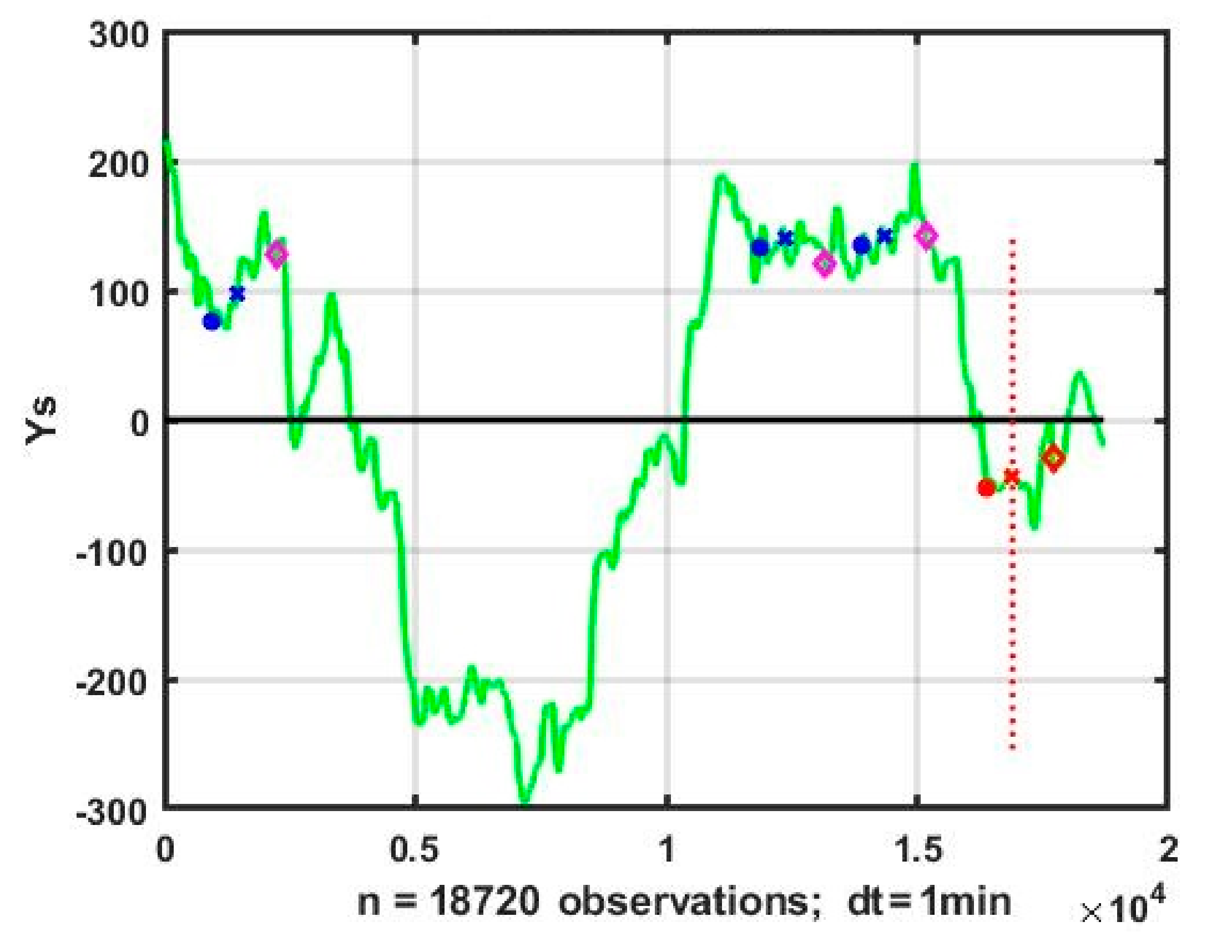
An example of selection of an analogous situation is shown in Figure 1. The vertical red line marks the zone of retrospective data used to generate a precedent prediction from the working zone on which the algorithm is tested. Beginnings and ends of intervals corresponding to the current situation and analogs are marked with stars and crosses, prediction values—with diamonds. The first analog shows an upward trend, which has already passed its maximum and demonstrates downward signs, while the second and third analogues have an unstable sideway. It is reasonable to avoid making predictive decisions and, if necessary, to conclude about a sideway (i.e., no obvious upward or downward trend).
From the perspective of machine learning, the proposed approach represents a solution of the forecasting problem based on weak machine classifiers. Low efficiency of classifiers is connected with the nature of observation time series, including chaotic system component and non-stationary random noises.
Figure 2 shows the expanded charts of the current state window (Figure 2a) and analog windows (Figure 2b–d). The solid lines in Figure 2b–d represent analogs to the chart in Figure 2a, which is imposed with a dot line. It allows for graphical verification of the problem solution, based on square metrics. The window in Figure 2b is a precedent, obtained using the k-NN method, i.e., it has the greatest similarity to the current situation presented in the Figure 2a. In this case, the degree of similarity is estimated with the measure (2).
For quality improvement it is necessary to obtain the degree of similarity for different analogs. In particular, the second analog (Figure 1), provides a poor prediction quality because its degree of similarity is only 0.49. This means that preliminary definition of the numbers of analog situations for non-stationary processes does not improve the quality of the forecast. Therefore, the method should be supplemented with the second level analog selection defined by allowed similarity threshold.
On the other hand, it is necessary to consider the size of the forecast interval for a given class of processes. Obviously, reducing of a forecast interval allows the acquisition of more accurate results. For example, reducing the forecast interval from 200 to 100 counts allowed for a reduction in the prediction error in the considered example by 17.5% and to get a quite satisfactory solution for the task being solved.
However, reducing the forecast time is not always acceptable. For example, by estimation of quality parameters of the output flow in a technological process by values of state parameters, the forecast interval is determined by the production structure and cannot be modified.
Improvement of prediction quality can be achieved by using a system of distributed forecasters based on weak classifiers with subsequent joint processing. The classifiers based on (3)–(5) can be used independently, with the solution chosen to match the forecasting scheme with the most accurate prediction in the sliding observation area.
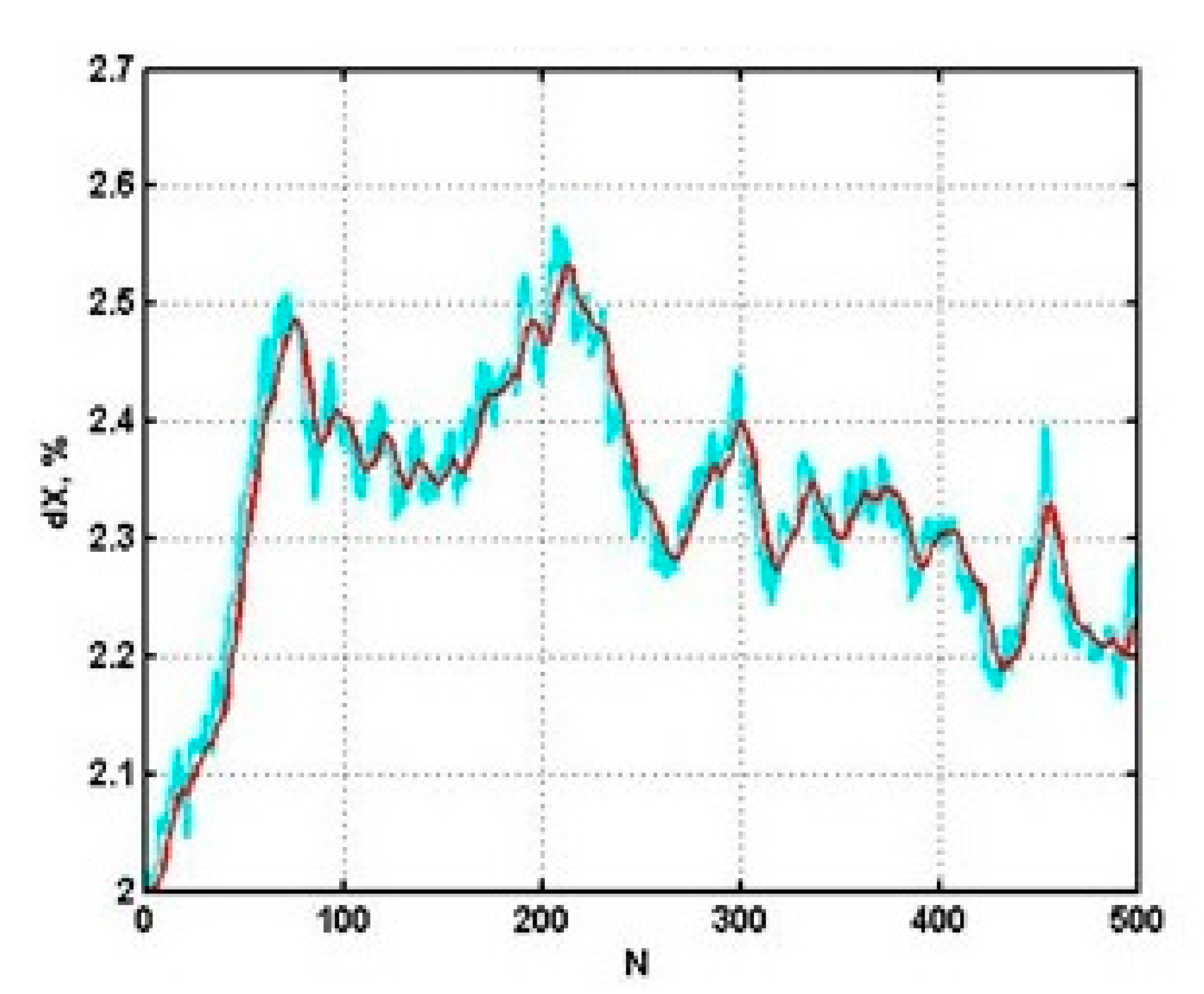
This scheme allows for the acquisition of quite satisfactory results for a certain class of applied tasks. For example, current temperature can be well predicted in a flow tube reactor used for production of aromatic hydrocarbons (Figure 3). At the same time the most frequent preference was given to the computational scheme with three closest neighbors with selection of analogs at the similarity level less than 50% and exponential smoothing with first order astatism and .
Within the limits of the considered scheme with nonstationary dynamics and chaotic system component, numerical comparison of quality of the prediction algorithms based on different variants of weak classifiers is possible. Variants of prognosis based on computational experiments can be formulated:
- P1. Precedent prediction (using the nearest-neighbor method) (3);
- P2. Average forecast based on three analogs (4);
- P3. Weighted average forecast using the three analogs (5);
- P4. Average forecast for analogs with similarity degree not lower than .
Four different one-day intervals (1440 counts) were considered. For each interval four variants of forecast P1–P4 were performed. The prediction quality was compared according to:
- Average absolute deviation
- Average square of deviations .
The values of the presented predictive quality indicators for four different one-day observation intervals and 4 prediction alternatives P1–P4 are presented in Table 1.
It can be seen that the forecast by a single precedent provides a lower accuracy than an average forecast by three analogs. The weighing of analogs in proportion to the degree of their similarity to precedent, practically affects the result compared to standard averaging. Additional selection of analogs at an acceptable similarity , decreased the accuracy of the forecast.
Thus, the variant with standard averaging of analogs was considered as the most preferable forecast strategy for the considered data. In this case the analogs with the size of the scanning window were used.
The presented values of prediction errors are quite high. Even in the best case for averaging based on three analogs the relative accuracy of the forecast varies around 10–25%. The reason for the low accuracy, is caused by the non-stationarity of the system noise and the chaotic nature of the observation time sequences.
The degree of prediction applicability with such accuracy is dependent on the task. In general, an increase in forecast accuracy is achieved by applying structural and parametric adaptation of the used algorithm. Structural adaptation can be reduced for selection of the most preferable number of analogs, from the database of retrospective observations.
The main advantage of the presented technique of forecasting nonstationary processes is the ability to detect and predict discontinuous changes in the controlled process. This possibility can be realized only if the accumulated data already contain changes, which need to be predicted.
For non-stationary dynamics of a more complex nature, which do not have mass or energy inertia (e.g., fast processes in microreactors with high controllability), it was impossible to make an effective prediction based on the considered computational scheme. Further studies based on examination of external factors and multidimensional statistical metrics are necessary.
4. Conclusions
The presented research allows one to substantiate the applicability of the precedent analysis for some classes of tasks for forecasting non-stationary flow processes with a chaotic system component. In particular, this technique is acceptable for processes with at least some inertia, such as technological processes in microreactors. However, for inertia-less processes, for example, generated by market quotes dynamics, such a prediction turns out to be unsuccessful. In this connection, further research in two directions is necessary:
- Building self-organizing forecasting algorithms which take into account changes in external factors affecting the controlled process;
- Application of multivariate analysis on the group of correlated processes using metrics of multivariate statistical analysis. In particular, the effectiveness of the precedent forecast based on the Mahalanobis distance, or other less common metrics such as the Hotelling’s trace or the Pillai’s trace is important.
Further development of the considered technique includes studies on predicting algorithm modification for non-stationary flow processes for multivariate correlated observation series.
Author Contributions
Conceptualization, A.M.; methodology, A.M.; software, E.B.; validation, A.M., E.B.; formal analysis, E.B.; investigation, A.M.; writing—original draft preparation, A.M.; writing—review and editing, E.B.; visualization, E.B.; supervision, E.B.; project administration, E.B.; funding acquisition, A.M., E.B. All authors have read and agreed to the published version of the manuscript.
Funding
This study was supported by the grants of Russian Fundamental Research Fund (No. 7-29-07073, 18-07-01272, 18-08-01505, 19–08–00989, 20-08-01046) in St. Petersburg Institute for Informatics and Automation of the Russian Academy of Sciences. Open Access Funding by the Publication Fund of the TU Dresden.
Conflicts of Interest
The authors declare no conflict of interest.
References
- Işığıçok, E.; Öz, R.; Tarkun, S. Forecasting and Technical Comparison of Inflation in Turkey With Box-Jenkins (ARIMA) Models and the Artificial Neural Network. Int. J. Energy Optim. Eng. (IJEOE) 2020, 9, 84–103. [Google Scholar] [CrossRef]
- Zhang, G.P. Time series forecasting using a hybrid ARIMA and neural network model. Neurocomputing 2003, 50, 159–175. [Google Scholar] [CrossRef]
- Peters, E. Simple and Complex Market Inefficiencies: Integrating Efficient Markets, Behavioral Finance, and Complexity. J. Behav. Financ. 2003, 4, 225–233. [Google Scholar] [CrossRef]
- Broer, H.W.; Simó, C.; Vitolo, R. Chaos and quasi-periodicity in diffeomorphisms of the solid torus. Discret. Contin. Dyn. Syst. Ser. B 2010, 14, 871–905. [Google Scholar] [CrossRef]
- Smith, L.A. Identification and prediction of low-dimensional dynamics. Phys. D 1992, 58, 50–76. [Google Scholar] [CrossRef]
- Cai, G.; Xue, L.; Zhang, H.; Lin, J. A Review on Micromixers. Micromachines 2017, 8, 274. [Google Scholar] [CrossRef] [PubMed]
- Wang, Y.; Zhe, J.; Dutta, P.; Chung, B.T. A microfluidic mixer utilizing electrokinetic relay switching and asymmetric flow geometries. J. Fluids Eng. 2007, 129, 399–403. [Google Scholar] [CrossRef] [Green Version]
- Box, G.; Hunter, W.; Hunter, J. Statistics for Experimenters: An Introduction to Design, Data Analysis, and Model Building, 2nd ed.; John Wiley & Sons: Hoboken, NJ, USA, 2005; 654p. [Google Scholar]
- Devore, J.; Farnum, N.; Doi, J. Applied Statistics for Engineers and Scientists, 3rd ed.; Cengage Learning: Boston, MA, USA, 2014. [Google Scholar]
- Bruce, P.; Bruce, A. Practical Statistics for Data Scientists; O’Reilly Media, Inc.: Sebastopol, CA, USA, 2017; 368p. [Google Scholar]
- Cérou, F.; Guyader, A. Nearest neighbor classification in infinite dimension. ESAIM Probab. Stat. 2006, 10, 340–355. [Google Scholar] [CrossRef] [Green Version]
- Larose, D.; Larose, C. Data Mining and Predictive Analysis; Wiley: Hoboken, NJ, USA, 2015. [Google Scholar]
- Schapire, R. The Strength of Weak Learnability. Mach. Learn. 1990, 5, 197–227. [Google Scholar] [CrossRef] [Green Version]
- Nguyen, H.D.; Wang, D.; McLachlan, G.J. Randomized mixture models for probability density approximation and estimation. Inf. Sci. 2018, 467, 135–148. [Google Scholar] [CrossRef] [Green Version]
Figure 1.
Example of the current widow and analog windows in the general time schedule of a smoothed process.
Figure 1.
Example of the current widow and analog windows in the general time schedule of a smoothed process.

Figure 2.
Window of the present position (a) and its corresponding analog windows (b–d).

Figure 3.
Relative accuracy of the prediction for the technological process with nonstationary dynamics.
Figure 3.
Relative accuracy of the prediction for the technological process with nonstationary dynamics.


Table 1.
Comparison of prediction quality indicators for four observation intervals.
| Observation Interval | Criterion | Prediction Alternative | |||
|---|---|---|---|---|---|
| P1 | P2 | P3 | P4 | ||
| 1 | 34.09 | 23.89 | 24.57 | 27.70 | |
| 2152.81 | 1054.82 | 1203.23 | 1673.13 | ||
| 2 | 35.00 | 19.52 | 19.54 | 29.60 | |
| 2416.21 | 589.28 | 624.98 | 1778.80 | ||
| 3 | 34.88 | 23.23 | 22.77 | 25.09 | |
| 2085.85 | 980.67 | 1019.16 | 1286.75 | ||
| 4 | 43.94 | 35.17 | 35.85 | 39.52 | |
| 3051.40 | 2087.24 | 2153.68 | 2559.02 | ||
© 2020 by the authors. Licensee MDPI, Basel, Switzerland. This article is an open access article distributed under the terms and conditions of the Creative Commons Attribution (CC BY) license (http://creativecommons.org/licenses/by/4.0/).
Share and Cite
MDPI and ACS Style
Musaev, A.; Borovinskaya, E. Prediction in Chaotic Environments Based on Weak Quadratic Classifiers. Symmetry 2020, 12, 1630. https://0-doi-org.brum.beds.ac.uk/10.3390/sym12101630
AMA Style
Musaev A, Borovinskaya E. Prediction in Chaotic Environments Based on Weak Quadratic Classifiers. Symmetry. 2020; 12(10):1630. https://0-doi-org.brum.beds.ac.uk/10.3390/sym12101630
Chicago/Turabian StyleMusaev, Alexander, and Ekaterina Borovinskaya. 2020. "Prediction in Chaotic Environments Based on Weak Quadratic Classifiers" Symmetry 12, no. 10: 1630. https://0-doi-org.brum.beds.ac.uk/10.3390/sym12101630
Note that from the first issue of 2016, this journal uses article numbers instead of page numbers. See further details here.