Divisibility Networks of the Rational Numbers in the Unit Interval

Abstract

Divisibility networks of natural numbers present a scale-free distribution as many other process in real life due to human interventions. This was quite unexpected since it is hard to find patterns concerning anything related with prime numbers. However, it is by now unclear if this behavior can also be found in other networks of mathematical nature. Even more, it was yet unknown if such patterns are present in other divisibility networks. We study networks of rational numbers in the unit interval where the edges are defined via the divisibility relation. Since we are dealing with infinite sets, we need to define an increasing covering of subnetworks. This requires an order of the numbers different from the canonical one. Therefore, we propose the construction of four different orders of the rational numbers in the unit interval inspired in Cantor’s diagonal argument. We motivate why these orders are chosen and we compare the topologies of the corresponding divisibility networks showing that all of them have a free-scale distribution. We also discuss which of the four networks should be more suitable for these analyses.

1. Introduction

Network science is the field that models different phenomena as networks of connected elements. There, the elements are represented by nodes which are connected by links or edges [1,2,3,4,5,6,7]. In recent years this has found applications and received contributions from a wide variety of research fields, such as telecommunications [8], machine learning [9], biology [10], social sciences [11], etc.

Recently, network science has been used to study mathematical properties from the point of view of complex systems apart from graph theory itself. Some interesting networks have arisen when studying mathematical structures of numbers sets: divisibility networks of natural numbers following the increasing sequential order, [12], divisibility networks of natural numbers according to its arrangement within the Pascal Triangle [13] or networks of prime numbers [14]. Yan et al. studied congruence relations through multiplex networks and studied the multiplex congruence network. They found that each one of the layers was sparse and presents a scale-free degree distribution [15].

This motivates our interest in studying how network measures can help us describe them and find hidden structures and hierarchies [16]. In some cases, we can even find analytical expressions of the results, as it is the case of the degree, clustering, geodesic distance, and centrality of the divisibility network on the natural numbers [17]. In addition. expressions for other centrality measures were shown in [18].

Network science has also provided an approach to analyze conjectures in number theory as it is the case of the Erdös–Straus conjecture [19] or the Goldbach conjecture [14]. Fibonacci networks were studied in [20], where the degree distribution and the average path length are calculated. These networks verify the small-world property and have an exponential degree distribution.

In this work, we study divisibility networks where the nodes are rational numbers, each of them connected to other nodes if one divides another one. Despite that we can find rational numbers at a different scale to natural numbers, we wonder if we rational numbers present symmetric behavior to the natural numbers with respect to the divisibility relation. We also consider that this approach of using network science data analysis tools on datasets of mathematical nature can attract the interest of pure mathematicians to these computational methods.

In principle, these networks consist of infinite sets of numbers (nodes). A common approach is to order the nodes and to define an increasing coverage of the set of nodes according to particular criteria to pick up the nodes. This approach permits to reduce an infinite network to an increasing family of subnetworks whose sets of nodes are in correspondence with the elements of the covering.

We say that a set A is countable if we can set a bijection $f:\mathbb{N}\to A$, which, in fact, also yields a sequential order on A, taking $a_1<a_2$, with $a_1,a_2\in A$, provided that $f^{-1}\left(a_1\right)<f^{-1}\left(a_2\right)$. Using again bijections, we can prove that the countable union of countable sets is again countable. So, to prove the countability of the rational numbers, it is enough to prove the countability of the rational numbers in the unit interval, and then to consider the countable union of intervals between consecutive integers.

In Section 2 we first propose the construction of four different types of networks in the unit interval that are based on Cantor’s diagonal argument. Later, we numerically analyze the structure of these networks. In Section 3, we study several topological parameters compared to the size of their respective subnetworks, and we see how do they evolve when the size of the network grows. In particular, we discuss the degree distribution $p\left(k\right)$; the local clustering coefficient $c\left(k\right)$; the average degree ${\langle k\rangle }_n$; the k cumulative degree; the local and global clustering coefficients $C_i$ and $C_{\Delta }$; the average clustering $\langle C\rangle$; the assortativity index r; the average path length $\langle d\rangle$, and the network density $\rho$. In particular, for the local clustering we represent it splitting the behavior for prime numbers in the numerator and in the numerator. Since the order of the rational numbers does not always correspond with the natural order in the interval, we also indicate their position according to the canonical order and the order obtained through different diagonal arguments. All these measures provide a general overview of the network structure and set the first steps for a more detailed analysis that can lead to conjecture analytic formulas that can describe this structure.

Finally, we present the conclusions and draft some future research lines.

2. Matherials and Methods

For studying the divisibility network of $\mathbb{Q}\cap ]0,1]$, we invoked Cantor’s diagonal argument to prove its countability [21]. He arranged all the rational numbers in an infinite-dimensional square matrix and he set a path there to order all their elements sequentially. In this work, we are going to consider several types of these matrices: In the first one, that we will call ${\mathcal{A}}^0=\left(a_{ij}^0\right)$, with $a_{ij}^0=i/j$ we arrange all positive rational numbers. It is explicitly given by:

$${\mathcal{A}}^0=\left\{\begin{array}{cccccccc}\hfill & \mathrm{Col}1& \mathrm{Col}2\hfill & \mathrm{Col}3& \mathrm{Col}4& \mathrm{Col}5& \mathrm{Col}5& \dots \\ \hfill \mathrm{Row}1& \mathbf{1}/\mathbf{1}& \mathbf{1}/\mathbf{2}\hfill & \mathbf{1}/\mathbf{3}& \mathbf{1}/\mathbf{4}& \mathbf{1}/\mathbf{5}& \mathbf{1}/\mathbf{6}& \dots \\ \hfill \mathrm{Row}2& \mathbf{2}/\mathbf{1}& \mathbf{2}/\mathbf{2}\hfill & \mathbf{2}/\mathbf{3}& \mathbf{2}/\mathbf{4}& \mathbf{2}/\mathbf{5}& 2/6& \dots \\ \hfill \mathrm{Row}3& \mathbf{3}/\mathbf{1}& \mathbf{3}/\mathbf{2}\hfill & \mathbf{3}/\mathbf{3}& \mathbf{3}/\mathbf{4}& 3/5& 3/6& \dots \\ \hfill \mathrm{Row}4& \mathbf{4}/\mathbf{1}& \mathbf{4}/\mathbf{2}\hfill & \mathbf{4}/\mathbf{3}& 4/4& 4/5& 4/6& \dots \\ \hfill \mathrm{Row}5& \mathbf{5}/\mathbf{1}& \mathbf{5}/\mathbf{2}\hfill & 5/3& 5/4& 5/5& 5/6& \dots \\ \hfill \mathrm{Row}6& \mathbf{6}/\mathbf{1}& 6/2\hfill & 6/3& 6/4& 6/5& 6/6& \dots \\ \hfill & ⋮& ⋮\hfill & ⋮& ⋮& ⋮& ⋮& \end{array}\right.$$

(1)

To order them sequentially, one just has to stack one right diagonal after the other. For every $n\in \mathbb{N}$, we define ${\mathcal{A}}_n^0$ as the list of numbers extracted from the first n-right diagonals of ${\mathcal{A}}^0$. For example, ${\mathcal{A}}_6^0$ will be

$${\mathcal{A}}_6^0=\left(\frac{1}{1},\frac{1}{2},\frac{2}{1},\frac{1}{3},\frac{2}{2},\frac{3}{1},\frac{1}{4},\frac{2}{3},\frac{3}{2},\frac{4}{1},\frac{1}{5},\frac{2}{4},\frac{3}{3},\frac{4}{2},\frac{5}{1},\frac{1}{6},\frac{2}{5},\frac{3}{4},\frac{4}{3},\frac{5}{2},\frac{6}{1}\right).$$

(2)

We start with the divisibility networks that have, as the set of nodes, all the non-repeated elements from ${\mathcal{A}}_n^0$, $n\in \mathbb{N}$. The corresponding set of nodes will be denoted by $V\left({\mathcal{A}}_n^0\right)$. For instance, $V\left({\mathcal{A}}_6^0\right)$ is

$$V\left({\mathcal{A}}_6^0\right)=\left\{\frac{1}{1},\frac{1}{2},\frac{2}{1},\frac{1}{3},\frac{3}{1},\frac{1}{4},\frac{2}{3},\frac{3}{2},\frac{4}{1},\frac{1}{5},\frac{5}{1},\frac{1}{6},\frac{2}{5},\frac{3}{4},\frac{4}{3},\frac{5}{2},\frac{6}{1}\right\}.$$

(3)

A connection between nodes, $v_i,v_j\in V\left({\mathcal{A}}_n^0\right)$ occurs if one divides the other, that is, the division is modulo 0 with a natural number as quotient. We remark that this will provide a non-directed network. We have also considered that one is connected with all the numbers, since it is the identity element for the division of non-null elements. We denote as $L\left({\mathcal{A}}_n^0\right)$ the set of links. The networks given by these sets of nodes and links will be denoted by $G\left({\mathcal{A}}_n^0\right)=(V\left({\mathcal{A}}_n^0\right),L\left({\mathcal{A}}_n^0\right))$. As an example, we plot in Figure 1 the network $G\left({\mathcal{A}}_6^0\right)$, which has 17 nodes, since $2/2$ and $3/3$ are equivalent to 1, $2/4$ is equivalent to $1/2$, and $4/2$ is equivalent to 2.

This first network based on Cantor’s diagonal argument will inspire the four networks that we will study here. In contrast to $G\left({\mathcal{A}}_n^0\right)$ that is a network of rational numbers, we will consider four different networks, all their elements will belong to $\mathbb{Q}\cap ]0,1]$.

2.1. Networks $G\left({\mathcal{A}}_n^1\right)$

The first type of network is denoted by $G\left({\mathcal{A}}_n^1\right)=(V\left({\mathcal{A}}_n^1\right),L\left({\mathcal{A}}_n^1\right))$, $n\in \mathbb{N}$. It is obtained directly from ${\mathcal{A}}_n^0$ by dividing all the nodes by the maximum number, which is n. This normalization rescales all numbers to fit within the unit interval without affecting the existing links between nodes. For example, from $V\left({\mathcal{A}}_6^0\right)$ one will obtain that the set of nodes $V\left({\mathcal{A}}_6^1\right)$ will be

$$V\left({\mathcal{A}}_6^1\right)=\left\{\frac{1}{6},\frac{1}{12},\frac{1}{3},\frac{1}{18},\frac{1}{2},\frac{1}{24},\frac{1}{9},\frac{1}{4},\frac{2}{3},\frac{1}{30},\frac{5}{6},\frac{1}{36},\frac{1}{15},\frac{1}{8},\frac{2}{9},\frac{5}{12},1\right\}.$$

(4)

2.2. Networks $G\left({\mathcal{A}}_n^2\right)$

A second network $G\left({\mathcal{A}}_n^2\right)=(V\left({\mathcal{A}}_n^2\right),L\left({\mathcal{A}}_n^2\right))$, $n\in \mathbb{N}$, can be obtained from ${\mathcal{A}}_n^0$ if we just pick up the numbers in $]0,1]$ and their connections. Therefore, links between nodes will be also set according to the aforementioned divisibility relation, but the number of nodes and links in $G\left({\mathcal{A}}_n^2\right)$ is smaller than the number of nodes and links of $G\left({\mathcal{A}}_n^1\right)$. For example, the set of nodes with $n=6$ will be

$$V\left({\mathcal{A}}_6^2\right)=\left\{\frac{1}{1},\frac{1}{2},\frac{1}{3},\frac{1}{4},\frac{2}{3},\frac{1}{5},\frac{1}{6},\frac{2}{5},\frac{3}{4}\right\},$$

(5)

which can be compared with $V\left({\mathcal{A}}_6^1\right)$ in (4). For illustrating these definitions, Figure 2a,b represent $G\left({\mathcal{A}}_6^1\right)$ and $G\left({\mathcal{A}}_6^2\right)$, respectively.

2.3. Networks $G\left({\mathcal{B}}_n^1\right)$

The next two networks are based on a matrix ${\mathcal{B}}^0=\left(b_{ij}^0\right)$, with $b_{ij}=i/(j+(i-1))$ and $i,j\in \mathbb{N}$. By construction, this matrix only contains rational numbers in the unit interval. In this matrix, the n-right diagonal will have n as a common denominator and the first n natural numbers as numerators.

$${\mathcal{B}}^0=\left\{\begin{array}{cccccccc}\hfill & \mathrm{Col}1& \mathrm{Col}2\hfill & \mathrm{Col}3& \mathrm{Col}4& \mathrm{Col}5& \mathrm{Col}5& \dots \\ \hfill \mathrm{Row}1& \mathbf{1}/\mathbf{1}& \mathbf{1}/\mathbf{2}\hfill & \mathbf{1}/\mathbf{3}& \mathbf{1}/\mathbf{4}& \mathbf{1}/\mathbf{5}& \mathbf{1}/\mathbf{6}& \dots \\ \hfill \mathrm{Row}2& \mathbf{2}/\mathbf{2}& \mathbf{2}/\mathbf{3}\hfill & \mathbf{2}/\mathbf{4}& \mathbf{2}/\mathbf{5}& \mathbf{2}/\mathbf{6}& 2/7& \dots \\ \hfill \mathrm{Row}3& \mathbf{3}/\mathbf{3}& \mathbf{3}/\mathbf{4}\hfill & \mathbf{3}/\mathbf{5}& \mathbf{3}/\mathbf{6}& 3/7& 3/8& \dots \\ \hfill \mathrm{Row}4& \mathbf{4}/\mathbf{4}& \mathbf{4}/\mathbf{5}\hfill & \mathbf{4}/\mathbf{6}& 4/7& 4/8& 4/9& \dots \\ \hfill \mathrm{Row}5& \mathbf{5}/\mathbf{5}& \mathbf{5}/\mathbf{6}\hfill & 5/7& 5/8& 5/9& 5/10& \dots \\ \hfill \mathrm{Row}6& \mathbf{6}/\mathbf{6}& 6/7\hfill & 6/8& 6/9& 6/10& 6/11& \dots \\ \hfill & ⋮& ⋮\hfill & ⋮& ⋮& ⋮& ⋮& \end{array}\right.$$

(6)

Then, we define ${\mathcal{B}}_n^0$ as the set of elements in the first n right diagonals from ${\mathcal{B}}^0$, where $n\in \mathbb{N}$. For example, the elements of ${\mathcal{B}}_6^0$ are listed in (7).

$${\mathcal{B}}_6^0=\left(\stackrel{1^{th}diagonal}{\overbrace{\frac{1}{1}}}\mid \stackrel{2^{th}diagonal}{\overbrace{\frac{1}{2},\frac{2}{2}}}\mid \stackrel{3^{th}diagonal}{\overbrace{\frac{1}{3},\frac{2}{3},\frac{3}{3}}}\mid \stackrel{4^{th}diagonal}{\overbrace{\frac{1}{4},\frac{2}{4},\frac{3}{4},\frac{4}{4}}}\mid \stackrel{5^{th}diagonal}{\overbrace{\frac{1}{5},\frac{2}{5},\frac{3}{5},\frac{4}{5},\frac{5}{5}}}\mid \stackrel{6^{th}diagonal}{\overbrace{\frac{1}{6},\frac{2}{6},\frac{3}{6},\frac{4}{6},\frac{5}{6},\frac{6}{6}}}\right).$$

(7)

Then, the third type of networks, denoted by $G\left({\mathcal{B}}_n^1\right)=(V\left({\mathcal{B}}_n^1\right),L\left({\mathcal{B}}_n^1\right))$, $n\in \mathbb{N}$ will have the non-repeated elements of ${\mathcal{B}}_n^0$ as the set of nodes. The set of links will again be given by the divisibility relation. As an example, the set of nodes for $n=6$ is

$$V\left({\mathcal{B}}_6^1\right)=\left\{\frac{1}{1},\frac{1}{2},\frac{1}{3},\frac{2}{3},\frac{1}{4},\frac{3}{4},\frac{1}{5},\frac{2}{5},\frac{3}{5},\frac{4}{5},\frac{1}{6},\frac{5}{6}\right\}.$$

(8)

2.4. Networks $G\left({\mathcal{B}}_n^2\right)$

Finally, we define a fourth type of network, denoted by $G\left({\mathcal{B}}_n^2\right)=(V\left({\mathcal{B}}_n^2\right),L\left({\mathcal{B}}_n^2\right))$, $n\in \mathbb{N}$, whose set of nodes ${\mathcal{B}}_n^2$ consists of the elements just in the n-th right diagonal of ${\mathcal{B}}_k^0$. Again, the sets of links $L\left({\mathcal{B}}_n^2\right)$ is given by the divisibility relation. For example, for $n=6$ one has

$$V\left({\mathcal{B}}_6^2\right)=\left\{\frac{1}{6},\frac{2}{6},\frac{3}{6},\frac{4}{6},\frac{5}{6},\frac{6}{6}\right\}.$$

(9)

We recall that in the first three types of networks, the set of nodes provides a covering of the rational numbers in the unit interval, excluding 0. However, in this fourth case, the set of nodes $V\left({\mathcal{B}}_n^2\right)$, $n\in \mathbb{N}$ is in correspondence with the first n-natural numbers. Note that when running n, one obtains an increasing family of networks isomorphic to the partial subnetworks of the divisibility network of natural numbers, which were analyzed in [12]. We represent examples of these last two types of networks in Figure 3, where we plot $G\left({\mathcal{B}}_6^i\right)$ for $i=1,2$.

3. Results

Since the matrices ${\mathcal{A}}^0$ and ${\mathcal{B}}^0$ are infinite dimensional, we take finite subnetworks of the different four types described above. We start analyzing the complexity of the network through the number of edges. As we have stated previously, despite considering a similar number of diagonals in matrix ${\mathcal{A}}^0$ and ${\mathcal{B}}^0$, the number of nodes and edges is different for each type of network. For a fixed number of diagonals, the networks $G\left({\mathcal{A}}_n^1\right)$ and $G\left({\mathcal{B}}_n^1\right)$ have more edges and nodes than the respective networks $G\left({\mathcal{A}}_n^2\right)$ and $G\left({\mathcal{B}}_n^2\right)$. The variation of their number of links is a key characteristic that will determine their degree distribution, as the comparative analysis we will carry out will show.

3.1. Degree Distribution

Let us consider an arbitrary network $G=(V,L)$, with V the set of nodes and L the set of edges. We denote by $\left|V\right|$ and $\left|L\right|$ the cardinals of both sets. We recall that the degree of a node $v\in V$ is the number of links adjacent to v. We denote by $p\left(k\right)$, $k\in \mathbb{N}$ the frequency with which nodes of degree k appear in G. That is, for every $k\in \mathbb{N}$ one has to count how many nodes have degree k, which we will denote as $N\left(k\right)$, and divide this number by the size of the set of nodes $\left|V\right|$, in order to obtain the fraction of nodes in the network with degree k, i.e., $p\left(k\right)=N\left(k\right)/\left|V\right|$. This can be illustrated with the histograms of the degree frequency, the cumulative degree, and the average degree $\langle k\rangle =2\left|L\right|/\left|V\right|$.

In order to better compare the densities, we compute a network of each type with $N=2^{16}$ nodes. We plot in Figure 4 the histogram of the degree distribution $p\left(k\right)$ with logarithmic bining ([5], Section 4.12.2) and the logfit to show that the number of links changes very differently for different networks.

These degree distributions are heavy tailed, similarly as it was shown in [12,13] for other divisibility networks. These distributions show a plateau for the frequencies of high-order degrees, Ref. ([5], Chapter 4.12.2). These distributions can be fitted to a power law distribution of the form $p\left(k\right)=C·k^{-\gamma }$, for all $k\ge k_{min}$. For each type of network we have estimated the values of $k_{min}$ and $\gamma$ through bootstrapping after 500 iterations. The results for $n=2^{16}$ are shown in Figure 4. On the one hand, the $k_{min}$ values median are: $k_{min}\left(G\left({\mathcal{A}}_n^1\right)\right)=4$, $k_{min}\left(G\left({\mathcal{A}}_n^1\right)\right)=1$, $k_{min}\left(G\left({\mathcal{B}}_n^1\right)\right)=4$, and $k_{min}\left(G\left({\mathcal{B}}_n^2\right)\right)=2$. We also see that the $\gamma$ estimations for two of the networks are very similar: $\gamma \left(G\left({\mathcal{A}}_n^1\right)\right)=2.05$ and $\gamma \left(G\left({\mathcal{B}}_n^2\right)\right)=2.03$. The other two networks provide higher values of $\gamma$, i.e., $\gamma \left(G\left({\mathcal{A}}_n^2\right)\right)=2.58$ and $\gamma \left(G\left({\mathcal{B}}_n^1\right)\right)=2.36$. We recall that for free scale networks, the $\gamma$ of the power-law fitting usually fulfills $2<\gamma <3$, which is satisfied for all the values obtained for $\gamma$. So that, according to these degrees distribution, we have that $G\left({\mathcal{A}}^1\right)$ is the divisibility network with a more similar behaviour to the divisibility network of the natural numbers, $G\left({\mathcal{B}}^2\right)$.

Alternatively, we can see how the number of edges increase through the k-cumulative degree or the average degree $\langle k\rangle$ in Figure 5a,b, respectively. There are some differences up to $n={10}^3$. However, from this value, the accumulated degrees tend to behave similarly. We see that network that $G\left({\mathcal{A}}^1\right)$ presents the highest average degree, and the others present similar values for big network sizes.

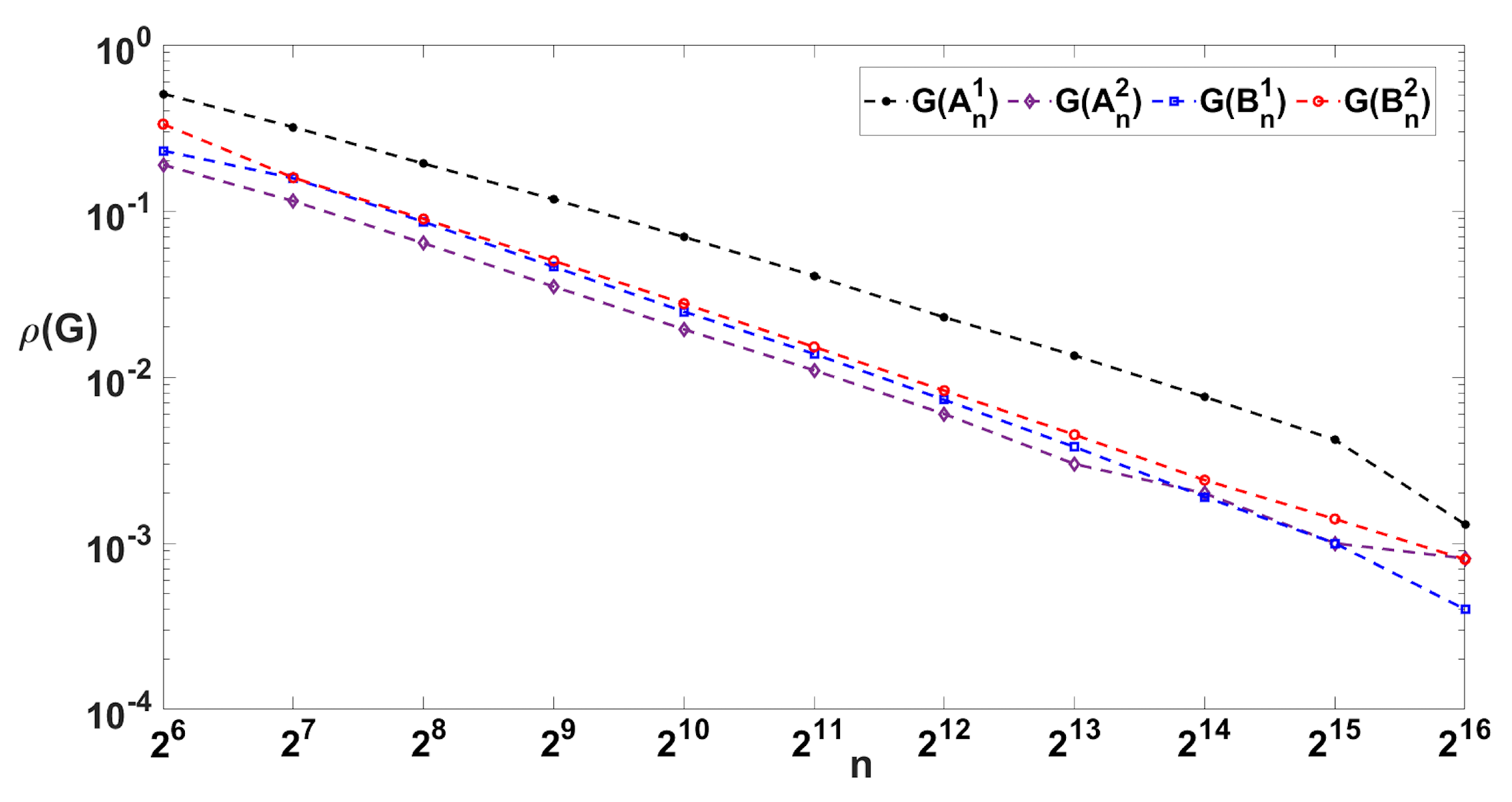
3.2. Density and Sparsity

Given a network $G=(V,L)$, we define its density $\rho \left(G\right)$ as the probability of a connection between an arbitrary pair of nodes in G. We compute it as the number of edges of the network divided by the maximum admissible number of edges that this network can have. In other words, $\rho \left(G\right)=\frac{2\left|E\right|}{\left|V\right|\left(\right|V|-1)}$, see for instance ([3], Chapter 6.10.1). This value ranges between $0\le \rho \le 1$, the closer to 0, the more sparse the network is, and the closer to 1, the denser it is. For $\rho =0$ we have the null network, and for $\rho =1$ we have a complete network.

In Figure 6, we appreciate that the density of $G\left({\mathcal{A}}^1\right)$ is higher than the others, which agrees with what we observed concerning the average and k-cumulative degrees.

3.3. Local Clustering Coefficient

The clustering coefficient can be interpreted as the coefficient that captures the degree to which the neighbors of a given node link to each other ([5], Chapter 2.10). Mathematically, the clustering coefficient of a degree $v_i\in V$ is computed as:

$$C_i=\frac{2L_i}{k_i(k_i-1)},$$

(10)

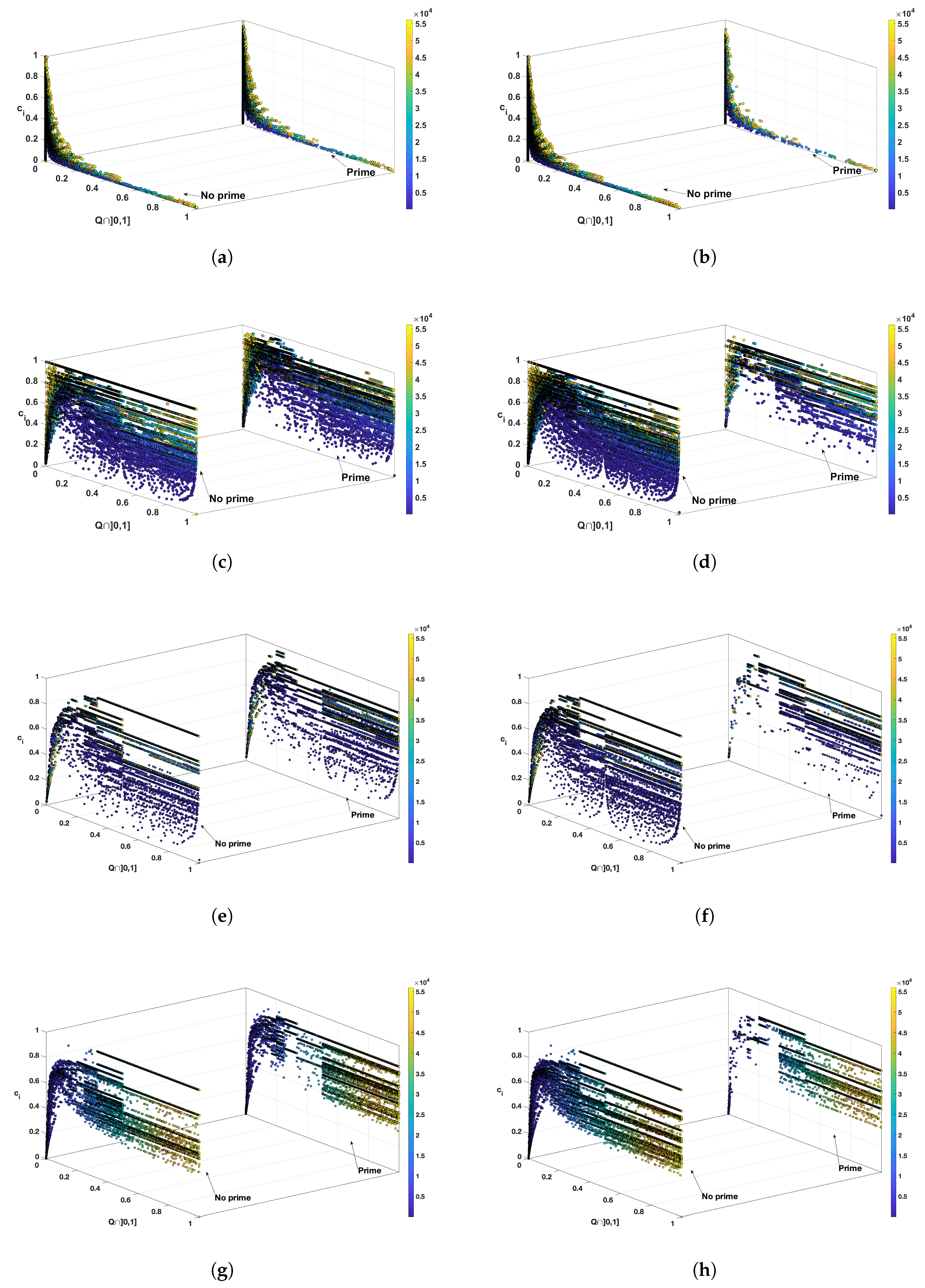
where $d\left(v_i\right)=k_i$ and $L_i\subset L$ is the set of edges connecting adjacent nodes to $v_i$ between them. The local clustering coefficient ranges between 0 and 1. It can also be understood as the probability that any two adjacent nodes to $v_i$ are connected by an edge. This probability gives us information about the density of links in the subnetwork given by the set of nodes adjacent to $v_i$. We have represented the stretching separating the cases in which the numerators and denominators are prime or not.

Unlike the results of [12,13], we have plotted the local clustering separating the cases in which numerators (denominators) are prime or not. The nodes are following the order in which they appear following the diagonal argument in their respective matrices. The results are presented in Figure 7. The order in which the nodes appear is represented with colors according to the scale near to each figure. We have also studied if the appearance of prime numbers in the numerator or denominator provides any insight to the clustering coefficient or the similarity stretching, but this is not the case, as we can see in Figure 7. With these networks, the behaviour more similar to $G\left({\mathcal{B}}^2\right)$ is given by $G\left({\mathcal{A}}^2\right)$ and $G\left({\mathcal{B}}^1\right)$.

3.4. Network Topologies

In this section we study four topological parameters: the global clustering coefficient, $C_{\Delta }$, the average clustering coefficient, $\langle C\rangle$, the assortativity coefficient, r, and the average path length, $\langle d\rangle$. Further details in ([3], Chapter 6) and ([5], Chapter 4).

3.4.1. Global Clustering Coefficient

The global clustering coefficient measures the degree of clustering of the whole network. A triplet consists of three nodes of a given network that are connected by edges. If they are just connected by two edges the triplet is said to be open. If they are connected by three, the triplet is closed.

The global clustering coefficient, denoted by $C_{\Delta }$ is the quotient of the total number of closed triplets divided by the total number of triplets (open and closed).

$$C_{\Delta }=\frac{3\times \mathrm{number}\mathrm{of}\mathrm{closed}\mathrm{triplets}}{\mathrm{number}\mathrm{of}\mathrm{triplets}(\mathrm{open}\mathrm{and}\mathrm{closed})}.$$

(11)

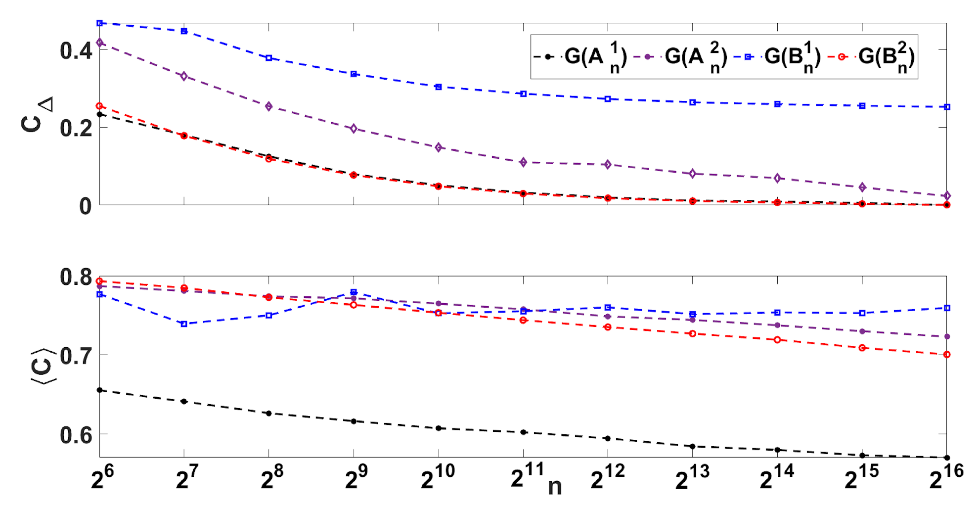
We see that it decreases to 0 as the size of the finite subnetworks of each type grow. It can be appreciated that $C_{\Delta }$ can be approximated by ${\displaystyle \frac{1}{N}}$ ([5], Chapter 4). Alternatively, in order to measure the clustering of the whole network one can also study the average clustering coefficient, $\langle C\rangle$, defined as the average of all local clustering coefficients of a network normalized by the network size, that is:

$$\langle C\rangle ={\displaystyle \frac{1}{\left|V\right|}}\sum _{i=1}^{\left|V\right|}{C}_i.$$

(12)

The comparison between both coefficients can be seen in Figure 8. We see that the global clustering coefficient tends to 0 as the size of the network gets bigger for all networks except for $G\left({\mathcal{B}}_n^1\right)$, which seems to stabilize around 0.3. On the contrary, the average clustering coefficient seems to be more inherent to the network and not so influenced by the network size. A significant difference is observed for the values of $G\left({\mathcal{A}}_n^1\right)$ respect to the other networks.

3.4.2. Assortative Coefficient

In order to measure how nodes are related between them, we compute the Pearson correlation between degrees of adjacent nodes, see for instance [22,23,24] or the more recent books ([3], Secetion 10.7) and [5]. The assortative coefficient of a given network is defined in (13).

$$r=\frac{{\sum }_{ij}(A_{ij}-k_i{k}_j/2\left|L\right|k_i{k}_j)}{{\sum }_{ij}(k_i{\delta }_{ij}-k_i{k}_j/2\left|L\right|)k_i{k}_j},$$

(13)

where $k_i$ is the degree of $v_i$, $A_{ij}$ is the ${(i,j)}^{th}$ element of the adjacency matrix associated to the eventual connection between $v_i$ and $v_j$, $\left|L\right|$ is the total of links in the network, and ${\delta }_{ij}$ is the Kronecker delta. However, determining the assortativity from (13) supposes a high computational cost, and therefore it is suggested to approximate the assortativity by means of the expression

$$r=\frac{S_1{S}_e-S^2}{S_1{S}_3-S_2^2}\mathrm{with}{S}_e=\sum _{ij}{A}_{ij}{k}_i{k}_j=2\sum _{l_{(i,j)}}{k}_i{k}_j,\mathrm{and}{S}_m=\sum _{i=1}^{N_n}{k}_i^m\mathrm{for}m=1,2,3,$$

(14)

where we have introduced $l_{(i,j)}$ for referring to all unordered pairs of nodes connected by an edge and $N_n$ is the total number of nodes of each one of our networks.

The assortativity coefficient presents values between $-1$ and 1. If $r=1$, we called the network to be fully assortative. In case of $r=0$ the network is said to be not assortative, while if $r=-1$, the network is called disassortative. The results can be seen in Figure 9. In the four cases, we find a non-assortative pattern that combines with the free-scale property emphasizes that highly connected nodes tend to connect with nodes of low degree.

On the other hand, we observe that the network is disassortative, $r<1$, and therefore the probability that there are clusters of nodes with the same characteristics is minimal, however, we can see that the assortativity coefficient tends to zero for each network type as n grows. Finally, the average path length $\langle d\rangle \to 2$ as n grows.

3.4.3. Average Path Length

The network average path length, denoted by $\langle d\rangle$ is the averaged distance between all pairs of different nodes [5]. For each pair, the distance between them is given by the shortest path connecting them. Since one is connected with all the nodes, then the average path length would be lower than 2.

$$\langle d\rangle =\frac{1}{N(N-1)}\sum _{\begin{array}{c}i,j=1\\ i\ne j\end{array}}^{\left|V\right|}{d}_{i,j}.$$

(15)

In our complex networks, we can see that the $\langle d\rangle \to 2$ for all networks, which means that all of them are close to being bipartite.

4. Conclusions

The countability of the set of rational numbers shown by Cantor is one of the most striking elementary results in Mathematics. Starting from his idea of the diagonal arrangement of rational numbers in a matrix, we can propose there is no unique way to set a sequential order in the rational numbers, even in the interval $[0,1]$.

We have explored four possible arrangements and their subsequent divisibility networks in order to study divisibility properties from the point of view of Network Science. In all these works, when studying the degree distribution and other network properties, we notice characteristics and structures similar to real based networks.

In all the cases, the obtained results agree with similar results presented by the natural numbers divisibility network explored in [12,13], holding the scale-free property again. We have seen that $G\left({\mathcal{A}}^1\right)$ behaves in a similar way as $G\left({\mathcal{B}}^2\right)$. We have also shown how different measures evolve with the network size, and the average path length seems to stabilize in 2, being close to what it yields for a bipartite network. The global clustering coefficient approaches to 0, except for the case of $G\left({\mathcal{B}}_n^1\right)$, which seems to give a value around 0.3. However, for the rest of the properties, $G\left({\mathcal{A}}^2\right)$ seems to present more similar characteristics to $G\left({\mathcal{B}}^2\right)$, the divisibility network of the natural numbers.

We can find many sequences and arrangements of countable sets in the development of mathematical results, which are susceptible to constructing networks linking them, as we have done here with the divisibility relation. We can also consider other relations among natural or rational numbers that would provide us with network coverage of the whole network. We consider of interest to know which are the underlying network topologies in each case. Moreover, we also wonder if we can find some analytical results that would back the obtained results. Besides, we also wonder if this approach can give further insight in order to state and prove new properties of the relationship under consideration.

References

- Watts, D.J. Small Worlds: The Dynamics of Networks Between Order And Randomness; Princeton University Press: Princeton, NJ, USA, 2004; Volume 9. [Google Scholar]
- Pastor-Satorras, R.; Rubi, M.; Diaz-Guilera, A. Statistical Mechanics of Complex Networks; Springer Science & Business Media: Berlin, Germany, 2003; Volume 625. [Google Scholar]
- Newman, M. Networks; Oxford University Press: Oxford, UK, 2018. [Google Scholar]
- Barrat, A.; Barthelemy, M.; Vespignani, A. Dynamical Processes on Complex Networks; Cambridge University Press: Cambridge, UK, 2008. [Google Scholar]
- Barabási, A. Network Science; Cambridge University Press: Cambridge, UK, 2016. [Google Scholar]
- Brandes, U.; Freeman, L.; Wagner, D. Social Networks; CRC Press: Boca Raton, FL, USA, 2013. [Google Scholar]
- Estrada, E. The Structure of Complex Networks: Theory and Applications; Oxford University Press: Oxford, UK, 2012. [Google Scholar]
- Jian, F.; Dandan, S. Complex network theory and its application research on P2P networks. Appl. Math. Nonlinear Sci. 2016, 1, 45–52. [Google Scholar] [CrossRef] [Green Version]
- Pérez-Benito, F.J.; García-Gómez, J.; Navarro-Pardo, E.; Conejero, J. Community detection-based deep neural network architectures: Afully automated framework based on Likert-scale data. Math. Methods Appl. Sci. 2020, 43, 8290–8301. [Google Scholar] [CrossRef]
- Barabasi, A.; Oltvai, Z. Network biology: Understanding the cell’s functional organization. Nat. Rev. Gen. 2004, 5, 101–113. [Google Scholar] [CrossRef] [PubMed]
- Borgatti, S.; Mehra, A.; Brass, D.; Labianca, G. Network analysis in the social sciences. Science 2009, 323, 892–895. [Google Scholar] [CrossRef] [PubMed] [Green Version]
- Shekatkar, S.M.; Bhagwat, C.; Ambika, G. Divisibility patterns of natural numbers on a complex network. Sci. Rep. 2015, 5, 14280. [Google Scholar] [CrossRef] [PubMed] [Green Version]
- Solares-Hernández, P.; Manzano, F.; Pérez-Benito, F.; Conejero, J. Divisibility patterns within Pascal divisibility networks. Mathematics 2020, 8, 254. [Google Scholar] [CrossRef] [Green Version]
- Chandra, A.; Dasgupta, S. A small world network of prime numbers. Phys. A Stat. Mech. Appl. 2005, 357, 436–446. [Google Scholar] [CrossRef] [Green Version]
- Yan, X.Y.; Wang, W.X.; Chen, G.R.; Shi, D.H. Multiplex congruence network of natural numbers. Sci. Rep. 2016, 6, 23714. [Google Scholar] [CrossRef] [PubMed] [Green Version]
- Bunimovich, L.; Smith, D.; Webb, B. Finding hidden structures, hierarchies, and cores in networks via isospectral reduction. Appl. Math. Nonlinear Sci. 2019, 4, 225–248. [Google Scholar] [CrossRef] [Green Version]
- Abiya, R.; Ambika, G. Patterns of primes and composites on divisibility graph. arXiv 2020, arXiv:2010.12153. [Google Scholar]
- Rajans, A.; Ambika, G. Patterns of primes and composites from divisibility network of natural numbers. arXiv 2020, arXiv:2007.00769. [Google Scholar]
- Mondreti, V. A Complex Networks Approach to Analysing the Erdös-Straus Conjecture and Related Problems. Preprint 2019. [Google Scholar] [CrossRef]
- Jing-Yuan, Z.; Wei-Gang, S.; Li-Yan, T.; Chang-Pin, L. Topological properties of Fibonacci networks. Commun. Theor. Phys. 2013, 60, 375. [Google Scholar]
- Vallin, R. The Elements of Cantor Sets: With Applications; Wiley Online Library: Hoboken, NJ, USA, 2013. [Google Scholar]
- Newman, M. Assortative mixing in networks. Phys. Rev. 2002, 89, 208701. [Google Scholar] [CrossRef] [PubMed] [Green Version]
- Newman, M. Mixing patterns in networks. Phys. Rev. 2003, 67, 026126. [Google Scholar] [CrossRef] [PubMed] [Green Version]
- Dorogovtsev, S.; Mendes, J. Evolution of networks. Adv. Phys. 2002, 51, 1079–1187. [Google Scholar] [CrossRef] [Green Version]
Figure 1.
Divisbility network , with 17 nodes and 71 links.
Figure 2.
Divisibility networks and . (a) The first one has 17 nodes and 71 links. (b) The second one has 9 nodes and 15 links.
Figure 3.
Divisibility networks and . The network in (a) has 12 nodes and 22 links and the network in (b) has 6 nodes and 10 links.
Figure 4.
Degree distribution with log-binning for the networks: (a) , (b) , (c) , (d) for a fixed network size of nodes.
Figure 5.
Evolution of the (a) k-cumulative and (b) for the networks , , , and for different network sizes up to nodes.
Figure 6.
Evolution of the density of networks , , and for different network sizes up to nodes.
Figure 7.
Local clustering coefficient of the networks (a,b) , (2nd row) , (c,d) , and (e,f) (g,h). On the left (right), we separate the values taking into account if the values of the numerator (denominator) are prime or not. Values are colored according to the order of the number following the diagonal argument on the corresponding matrix.
Figure 8.
Evolution of the global clustering coeffcient, , and the average clustering coefficient , for different network sizes up to .
Figure 9.
Evolution of the assortativity coefficient, r, and the average path length, , for different network sizes.
Publisher’s Note: MDPI stays neutral with regard to jurisdictional claims in published maps and institutional affiliations. |
© 2020 by the authors. Licensee MDPI, Basel, Switzerland. This article is an open access article distributed under the terms and conditions of the Creative Commons Attribution (CC BY) license (http://creativecommons.org/licenses/by/4.0/).
Share and Cite
MDPI and ACS Style
Solares-Hernández, P.A.; García-March, M.A.; Conejero, J.A. Divisibility Networks of the Rational Numbers in the Unit Interval. Symmetry 2020, 12, 1879. https://0-doi-org.brum.beds.ac.uk/10.3390/sym12111879
AMA Style
Solares-Hernández PA, García-March MA, Conejero JA. Divisibility Networks of the Rational Numbers in the Unit Interval. Symmetry. 2020; 12(11):1879. https://0-doi-org.brum.beds.ac.uk/10.3390/sym12111879
Chicago/Turabian StyleSolares-Hernández, Pedro A., Miguel A. García-March, and J. Alberto Conejero. 2020. "Divisibility Networks of the Rational Numbers in the Unit Interval" Symmetry 12, no. 11: 1879. https://0-doi-org.brum.beds.ac.uk/10.3390/sym12111879
Note that from the first issue of 2016, this journal uses article numbers instead of page numbers. See further details here.