Entropy Generation in a Mass-Spring-Damper System Using a Conformable Model

Abstract

This article studies the entropy generation of a mass-spring-damper mechanical system, under the conformable fractional operator definition. We perform several simulations by varying the fractional order $\gamma$ and the damping ratio $\zeta$, including the usual dynamic response when $\gamma =1.0$ and the typical damping cases. We analyze the entropy production for this system and its strong dependency on both $\gamma$ and $\zeta$ parameters. Therefore, we determine their optimal values to obtain the highest efficiency of the MSD response, as well as other impressive features.

1. Introduction

Mass-spring-damper (MSD) systems are vastly known as strong conceptual strategies for modeling purposes in diverse areas of knowledge. Their secret resides in their simplicity, which makes them ideal for modeling more complex systems by taking advantage of the modularity principle. The concept of an MSD system has been implemented on a vast number of practical fields, such as in the reduction of vibrations [1,2], in control systems analysis [3,4], and in power generation [5,6]. Those systems have been independently studied under different lenses, such as fractional calculus and entropy production. On the one hand, fractional calculus (FC) is a natural generalization of ordinary calculus. It deals with non-integer order derivatives and integrals. Specifically, fractional derivatives are non-local operators because they are defined by an integral, which gives them a memory effect in temporal applications that is useful for specific dynamic processes [7,8]. A glance at the development of fractional calculus shows a growing interest since the 1990s—that is, the Scopus database reported 168, 894, and 4765 scientific documents related to FC in the decades of 1990–1999, 2000–2009, and 2010–2019, respectively. Therefore, it is evident that FC is receiving great attention from the scientific community for modeling natural phenomena and nourishing current mathematics, just like Leibniz prophesied [9,10]. In the literature, several definitions of fractional derivatives and integrals have been proposed [8], including Riemann–Liouville, Grünwald–Letnikov, Caputo, Weyl [7,8,11], and more recently, Caputo–Fabrizio [12] and Atangana–Baleanu [13]. All these definitions satisfy the property of linearity. Still, properties such as the product, quotient, chain, and composition rules, as well as the mean value and Rolle’s theorems, to mention a few, are lacking in almost all fractional derivatives. To tackle these issues, Khalil et al. proposed an extension of the ordinary limit definition for the derivative of a function, namely, the conformable fractional derivative [14]. This definition allows the generalization of some classical theorems from the ordinary calculus, and therefore it has attracted the interest of researchers because it seems to satisfy all the standard derivative requirements [15]. It is clear that this derivative, unlike those mentioned before, is local. Additionally, the computing burden when using this operator is considerably lighter than when using other fractional derivative definitions. All these features have been corroborated in the literature, where there have been a large number of works carried out with this definition [16,17,18,19,20,21,22].

Nevertheless, FC is currently a trending topic in the scientific community with very interesting and recurrent discussions, as is expected, particularly about “Is the conformable operator a fractional derivative?”. Unfortunately, that is a matter beyond the scope of this work, cf. [19,23,24,25,26]. Henceforth and for the sake of politeness, we use the word “operator” instead of “derivative” to refer to the fractional conformable definition. Regarding the fractional derivative application in the modeling of MSD systems, the literature shows an increasing number of publications in the last decade. Achar et al. studied the motion of a harmonic oscillator and found a fractional model based on Mittag-Leffler functions through Laplace transforms [27]. Therefore, they analyzed its energy, response, and resonance characteristics under multiple scenarios, including different forcing functions [28,29]. Recently, Berman et al. solved a damped mechanical harmonic oscillator system with asymptotic behavior by employing the Caputo fractional derivative definition and Laplace transform [30]. Their solution showed an evident difference with respect to that for the standard oscillator. In contrast, the former presented an algebraic decay having a finite number of zeros. Thence, it was noticed that the fractional damped oscillator total energy depends on both time and fractional order. Still, when it depends only on time, it decreases faster than the standard one. On the other hand, entropy generation analysis (EGA), pioneered by Bejan in [31], is a strategy based on thermodynamic foundations to study and design real engineering systems [32]. EGA has received significant attention because it is based on the second law of thermodynamics and is capable of evaluating the energetic quality of a real process (i.e., how distant a system is from its ideal performance) [33]. Another essential fact about EGA is that it makes it possible to build a comprehensive model for a complex system as the sum of the entropy production contribution of all its components. Sunar et al. performed an analysis based on the entropy generation model for a typical MSD system [34].

In this paper, the fractional differential equation of the MSD system is obtained from the ordinary differential equation by employing the transformation method proposed in [35]. After that, a new class of ordinary linear differential equations with non-integer power variable coefficients is achieved under the conformable fractional operator definition. Then, a conformable model for the MSD system was coined and numerically simulated, assuming different cases of damping responses and fractional order. Several dynamic responses were analyzed using EGA and remarkable inferences are discussed about the influence of both the damping factor and the fractional order over the dynamic behavior and entropy production of the system. Thus, the following section presents basic concepts about the conformable operator and the entropy generation of mechanical systems. Subsequently, the corresponding mathematical models are described and analyzed using the most representative damping cases. Finally, results are discussed, and the most relevant conclusions are stated.

2. Preliminary

2.1. Conformable Fractional Operator

The conformable fractional operator, proposed by Khalil et al. [14], is described in the following definition.

Definition 1.

The γ-order conformable fractional form of a given function, $f(t):[0,\infty [\to \mathbb{R}$, is defined by

$$T_{\gamma }\{f\}(t)=\underset{ϵ\to 0}{\lim }\frac{f(t+ϵt^{1-\gamma })-f(t)}{ϵ},$$

(1)

since $t\ge 0$, and $\gamma \in ]0,1]$. Now, if $f(t)$ is γ-differentiable in some interval $t\in ]0,a[$, with $a>0$, and ${\lim }_{\tau \to 0^{+}}{\left.d^{\gamma }f/d{t}^{\gamma }\right|}_{t=\tau }$ exists, then one can define

$${\left.T_{\gamma }\{f\}(t)\right|}_{t=0}=\underset{\tau \to 0^{+}}{\lim }{\left.\frac{d^{\gamma }f}{d{t}^{\gamma }}\right|}_{t=\tau }.$$

(2)

The most important properties of this derivative are given in the following theorem [19,36].

Theorem 1.

Let $\gamma \in ]0,1]$, $a,b\in \mathbb{R}$ be constants and, $f(t)$ and $g(t)$ be γ-differentiable at a point $t>0$. Hence,

1.

$T_{\gamma }\{a\}(t)=0$;

2.

$T_{\gamma }\{t^b\}(t)=b·t^{b-\gamma }$;

3.

$T_{\gamma }\{a·f\pm b·g\}(t)=a·T_{\gamma }\{f\}(t)\pm b·T_{\gamma }\{g\}(t)$;

4.

$T_{\gamma }\{f\circ g\}(t)={\displaystyle \frac{df}{dg}}·T_{\gamma }\{g\}(t);$

5.

$T_{\gamma }\{f·g\}(t)=T_{\gamma }\{f\}(t)·g(t)+f(t)·T_{\gamma }\{g\}(t);$

6.

$T_{\gamma }\left\{f/g\right\}(t)={\displaystyle \frac{g(t)·T_{\gamma }\{f\}(t)-f(t)·T_{\gamma }\{g\}(t)}{g^2(t)}};$

7.

$T_{\alpha }\{f(t)\}=t^{n+1-\alpha }{\displaystyle \frac{d^{n+1}f}{d{t}^{n+1}}},\alpha \in ]n,n+1],n\in {\mathbb{Z}}_{+}$; and f is $(n+1)$-differentiable at $t>0$.

Thus, a simple extension of the ordinary derivative definition complies with most of the classical theorems in calculus, which is advantageous for different application fields.

2.2. Entropy Generation of Mechanical Systems

The behavior of any practical system in engineering can be described by the first and second laws of thermodynamics, which serve to analyze the quantity and quality of its process, respectively [32]. Its boundary defines an arbitrary closed system at T (K), delimiting it from the environment at $T_0$ (K) and acting as the interface for the energy and entropy interactions. These interactions either contribute to or result from the process carried out by the system. A simple process is defined between two equilibrium states I-II, where the system changes its energy ($\Delta E_{\text{I-II}}$ (J)) and entropy ($\Delta S_{\text{I-II}}$ (J/K)). At the same time, it exchanges energy and entropy with the surroundings, since $\delta Q$ (J), $\delta W$ (J), and $\delta Q/T$ (J/K) are the heat, work, and entropy transfer. Therefore, the first and second laws of thermodynamics for any closed practical system are written respectively as:

$${\int }_{\mathrm{I}}^{\mathrm{II}}(\delta Q+\delta W)=\Delta E_{\text{I-II}},$$

(3)

$${\int }_{\mathrm{I}}^{\mathrm{II}}\frac{\delta Q}{T}+S_{gen}=\Delta S_{\text{I-II}},$$

(4)

where $S_{gen}$ (J/K) is the entropy generated during the process I-II. $S_{gen}$ indicates the influence of irreversibilities, and it is inherent and always positive in real processes, since $S_{gen}=0$ J/K means idealness [32].

Plugging Equations (3) and (4) through $\delta Q$, and approaching the temperature distribution of the boundary to an average value, like the ambient temperature ($T=T_0$ (K)), it gives an explicit expression of the entropy generation ($S_{gen}$) for the operating system

$$S_{gen}=\Delta S_{\text{I-II}}+\frac{1}{T_0}\left({\int }_{\mathrm{I}}^{\mathrm{II}}\delta W-\Delta E_{\text{I-II}}\right).$$

(5)

It is important to recognize that the total energy change, $\Delta E_{\text{I-II}}$ in Equation (5), comprises energy changes of different nature. In the strict sense of mechanical systems, the formula in Equation (5) is simplified by assuming that: kinetic and potential energy changes ($\Delta K_{\text{I-II}}$ and $\Delta V_{\text{I-II}}$) are considered, and other types of energy changes are neglected; heat transfer leaving the system is generated due to irreversibilities; heat fluxes entering the system are disregarded; and entropy change and net produced work remain constant. Then, $S_{gen}$ in Equation (5) is rewritten as

$$S_{gen}=\Delta S_{\text{I-II}}+\frac{1}{T_0}\left({\int }_{\mathrm{I}}^{\mathrm{II}}\delta W-\Delta K_{\mathrm{I}-\mathrm{II}}-\Delta V_{\text{I-II}}\right).$$

(6)

However, energy measurements are difficult to obtain in a laboratory setup. So, instead of using Equation (6), a practical expression can be reached by applying a temporal differential operator, as follows,

$${\dot{S}}_{gen}=-\frac{1}{T_0}\left(\dot{K}+\dot{V}\right).$$

(7)

Equation (7) shows a direct relationship, known as the Gouy–Stodola theorem [32], between the entropy generation rate, ${\dot{S}}_{gen}$ (W/K), and the quotient of total power, $\dot{W}=(\dot{K}+\dot{V})$ (W), and ambient temperature, $T_0$ (K).

3. Mathematical Models

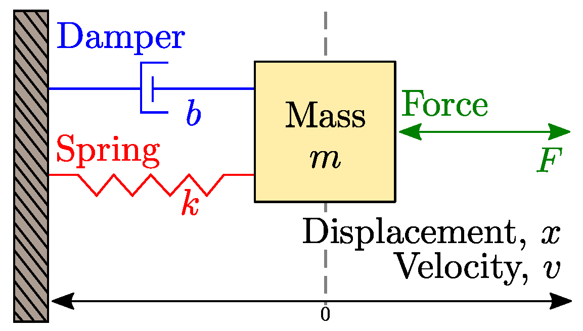
Figure 1 shows a simple mass-spring-damper (MSD) system, consisting of a mass (m (kg)) attached, simultaneously, to a linear spring with k (N/m) and a linear damper with b (N·s/m). An external force (F (N)) excites the system dynamic, which is characterized by the displacement (x (m)) and velocity (v (m/s)) of mass. However, this work studies the natural response of the MSD system (i.e., the external force is null), notwithstanding results and models presented here can be extended with ease.

3.1. Ordinary Model

The well-known ordinary differential equation (ODE) governing the MSD system (Figure 1) dynamics is:

$$m\frac{d^{2}x}{d{t}^2}+b\frac{dx}{dt}+kx=F(t),x(0^{+})=x_0,{\left.\frac{dx}{dt}\right|}_{t=0^{+}}=v_0,$$

(8)

since $x_0$ (m) and $v_0$ (m/s) are the initial conditions. Another common form to model this system is by using the natural frequency (${\omega }_n=\sqrt{k/m}$ (rad/s)) and the damping ratio ($\zeta =b/2\sqrt{km}$), such as,

$$\frac{d^{2}x}{d{t}^2}+2\zeta {\omega }_n\frac{dx}{dt}+{\omega }_n^{2}x=\frac{F(t)}{m},x(0^{+})=x_0,{\left.\frac{dx}{dt}\right|}_{t=0^{+}}=v_0.$$

(9)

From classical dynamic systems theory, the natural response of Equation (9) is defined by the complex frequency, which has four cases: the overdamped ($\zeta >1$), the critically damped ($\zeta =1$), the underdamped ($0<\zeta <1$), and the undamped ($\zeta =0$). The explicit solutions of Equation (9) are vastly studied in the literature, therefore, for the sake of brevity, this work does not detail them.

3.2. Fractional Model

To obtain a general fractional model for the MSD system, it is necessary to transform the ordinary model in Equation (9) into a fractional differential equation (FDE). That is possible by changing the ordinary derivative operator by a fractional one, in accordance with the procedure proposed by Rosales et al. in [35], as follows:

$$\frac{d^m}{d{t}^m}\to {\omega }_n^{m(1-\gamma )}\frac{d^{m\gamma }}{d{t}^{m\gamma }},\forall m\in {\mathbb{Z}}_{+},$$

(10)

where $\gamma \in ]0,1]$ is the fractional order. Applying Equation (10) in Equation (9), the resulting FDE is stated as

$$\frac{d^{2\gamma }x}{d{t}^{2\gamma }}+2\zeta {\omega }_n^{\gamma }\frac{d^{\gamma }x}{d{t}^{\gamma }}+{\omega }_n^{2\gamma }x={\omega }_n^{2(\gamma -1)}\frac{F(t)}{m}.$$

(11)

It is straightforward to notice that in the case $\gamma =1$, the FDE in Equation (11) is reduced to the ODE in Equation (9). This FDE has been studied using different definitions of fractional derivative [37,38,39]. However, most of them allow initial conditions that are difficult to fit into a physical meaning.

3.3. Conformable Model

Subsequently, taking into account the fractional derivative operators in Equation (10) and Theorem 1, an important operator change appears according to [40], as:

$$\underset{\mathrm{Ordinary}}{\underbrace{\frac{d^m}{d{t}^m}}}\to \underset{\mathrm{Fractional}}{\underbrace{{\omega }_n^{m(1-\gamma )}\frac{d^{m\gamma }}{d{t}^{m\gamma }}}}\to \underset{\mathrm{Conformable}}{\underbrace{{\omega }_n^{m(1-\gamma )}{t}^{m(1-\gamma )}\frac{d^m}{d{t}^m}}}.$$

(12)

Then, the FDE in Equation (11) can be formulated in the conformable sense, as shown:

$$\frac{d^{2}x}{d{t}^2}+2\zeta {\omega }_n^{\gamma }{t}^{\gamma -1}\frac{dx}{dt}+{\omega }_n^{2\gamma }{t}^{2(\gamma -1)}x={\omega }_n^{2(\gamma -1)}{t}^{2(\gamma -1)}\frac{F(t)}{m}.$$

(13)

This is a linear non-homogeneous differential equation with $\gamma$-powered variable coefficients, with the original initial conditions, which is easy to tackle using traditional procedures. Moreover, if $\gamma =1$ then the conformable model in Equation (13) becomes the ordinary model in Equation (8).

3.4. Entropy Production Rate Model

Finally, to determine the entropy production rate model using Equation (7), it is required to know the total energy of the MSD system (in Figure 1) without any external force ($F(t)=0$ N), given by

$$E(t)=\frac{1}{2}k{x}^2(t)+\frac{1}{2}m{v}^2(t),$$

(14)

since the squared terms of displacement ($x(t)$ (m)) and velocity ($v(t)$ (m/s)) are related to the potential ($V(t)$ (J)) and kinetic ($K(t)$ (J)) energies, respectively. Substituting Equation (14) into Equation (7), ${\dot{S}}_{gen}(t)$ has the form:

$${\dot{S}}_{gen}(t)=-\frac{m}{T_0}\left({\omega }_n^{2}x(t)+a(t)\right)v(t),$$

(15)

and replacing $a(t)=d^{2}x/d{t}^2$ (m/s²) from Equation (9) gives

$${\dot{S}}_{gen}(t)=\frac{2m}{T_0}\zeta {\omega }_n{v}^2(t)=\frac{b}{T_0}{v}^2(t).$$

(16)

This expression correlates the entropy generation rate ${\dot{S}}_{gen}$, the viscous damping constant b, the surrounding temperature $T_0$, and the system velocity $v(t)$. This expression agrees with the one reported by Sunar et al. in [34], where the process becomes reversible (${\dot{S}}_{gen}=0$ W/K) when the undamped case ($\zeta =0$) is studied.

4. Results and Discussion

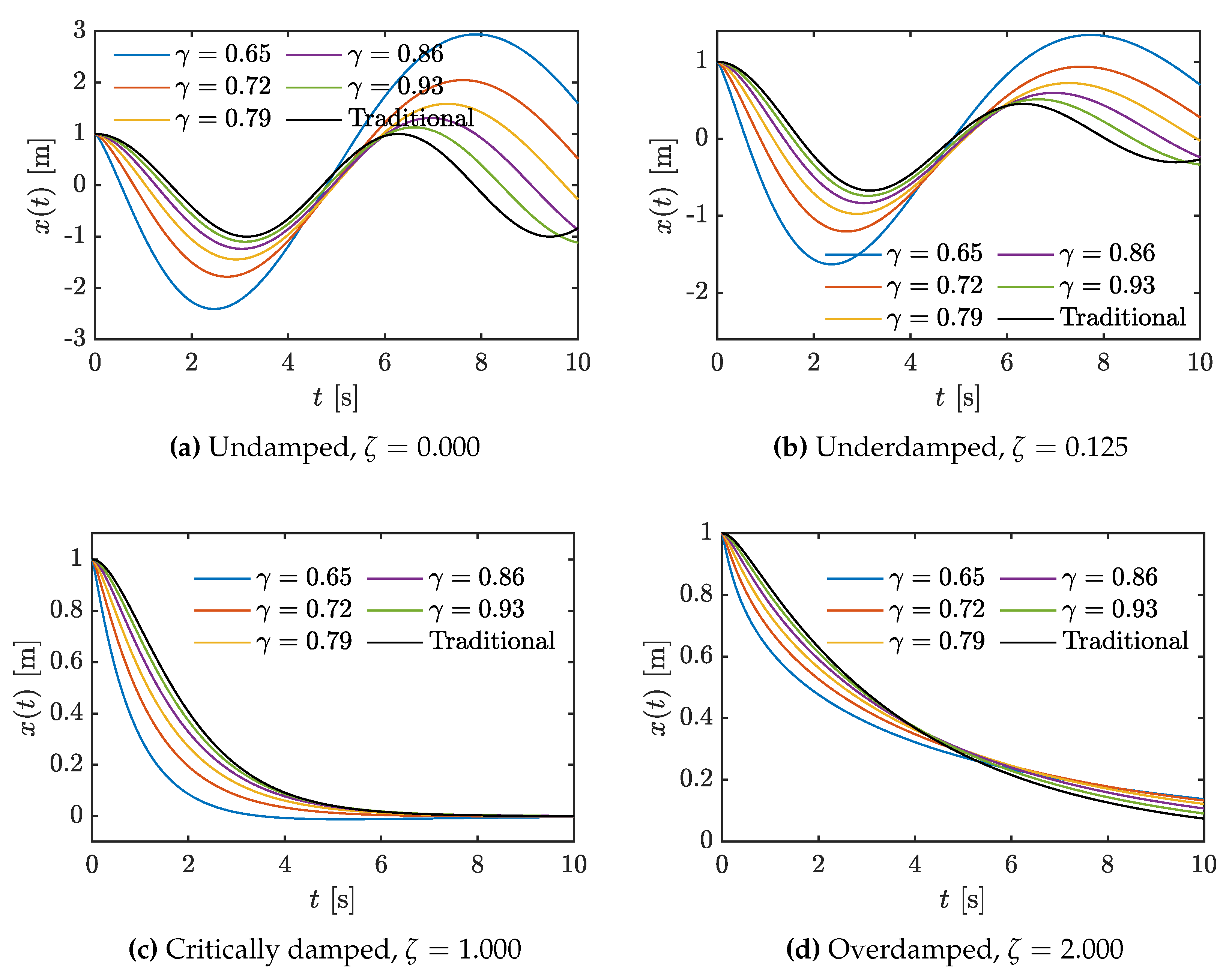
This work studied the natural response of the simple MSD system presented in Figure 1, using the conformable fractional derivative model developed in Equation (13), and its entropy generation rate obtained in Equation (16). Simulations were carried out considering a mass m of 1.0 kg, a natural frequency ${\omega }_n$ of 1.0 rad/s, an initial displacement $x_0$, and velocity $v_0$ of 1.0 m and 0.0 m/s, respectively, an ambient temperature $T_0$ of 298.15 K, a time span of 60 s with 500 samples, a null external force ($F(t)=0$ N), and different values of fractional order (i.e., $\gamma =0.65,0.72,\dots ,1.00$). Moreover, the damping ratio $\zeta$ determines the type of transient that an MSD system will exhibit, hence the values of $\zeta$ equal to $0.0,0.125,1.0$, and $2.0$ were selected to render the undamped, underdamped, critically damped, and overdamped cases, respectively.

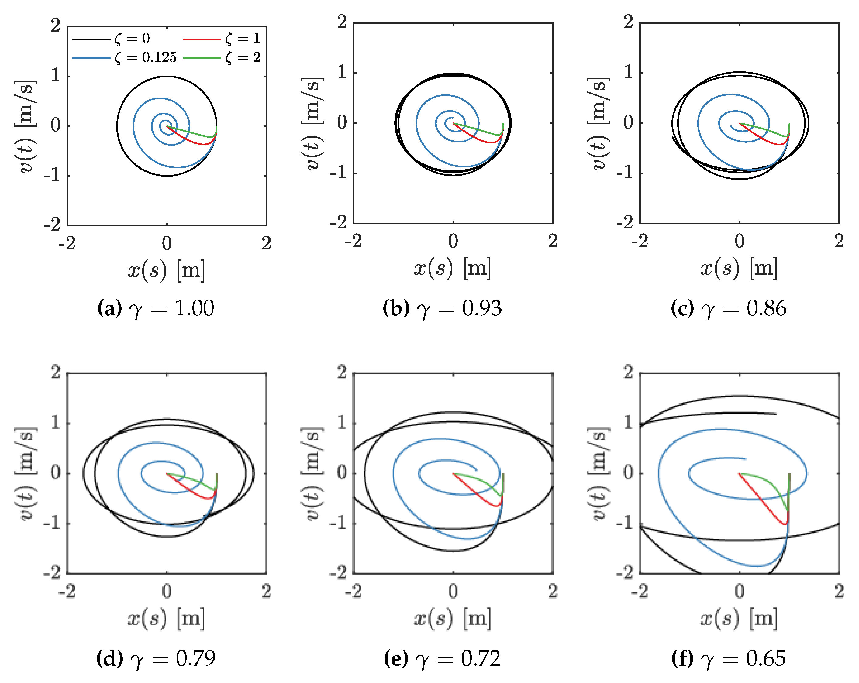
Figure 2 shows the displacement x of the MSD system in a time window of ten seconds, considering the four damping cases and varying the fractional order $\gamma$, including the traditional response (i.e., when $\gamma =1$). It is noticeable that the different displacement curves follow the traditional one, especially when the damping factor is increased. Responses with lower fractional orders have a greater magnitude of velocity, which is directly related to the kinetic energy. This can be validated with Figure 3, where the phase plane $x(t)$ vs. $v(t)$ is displayed for several values of $\gamma$. It is important to remark that $\gamma$ values greater than 0.6 avoid a divergent tendency of $x(t)$ (i.e., the model becomes unstable when the fractional order is decreased ($\gamma \to 0$)). In addition, defining $\gamma =0$ violates the conformable definition and has no sense in the dynamic system analysis. Moreover, when $\zeta =0$ in Figure 3, curves corroborates the free damped response.

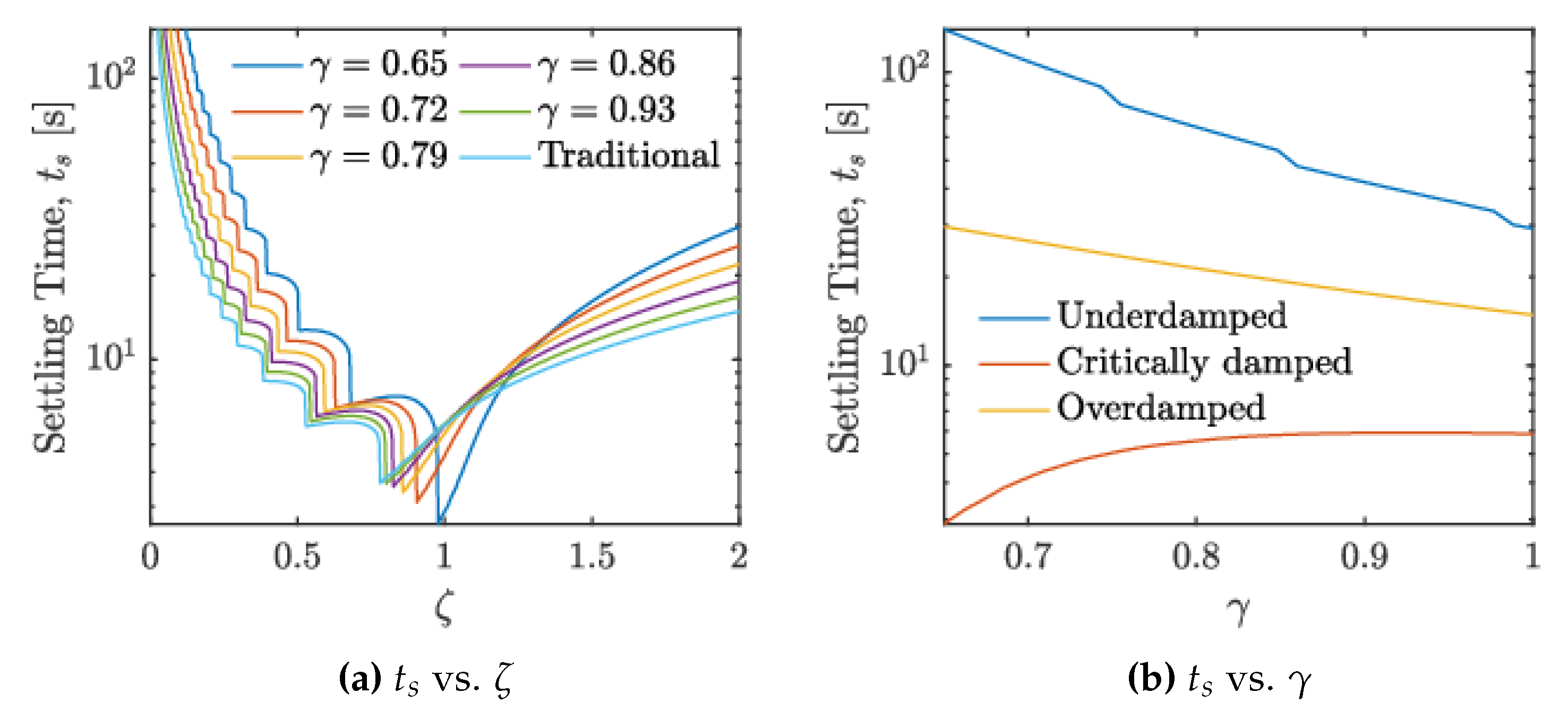
Figure 4 presents the influence of varying either the damping ratio $\zeta$ and the fractional order $\gamma$, over the settling time $t_s$ (s). Figure 4a shows that the minimal value of $t_s$ depends on $\zeta$ and $\gamma$, agreeing with the form,

$$t_{s,min}(\gamma ,\zeta )=11.33-1.474\gamma -7.967\zeta .$$

(17)

For the special case of $\gamma =1.00$ (the ordinary derivative), it is found that ${\zeta }^{\ast }=0.78$ minimizes the settling time, that is, ${\zeta }^{\ast }=\arg {\min }_{\zeta |\gamma =1}\{t_s(\zeta )\}$ with $t_{s,min}=t_s({\zeta }^{\ast })=3.64$ s. Likewise, Figure 4b illustrates the $t_s$ tendency while the fractional order increases, in the three defined damping cases. Moreover, the time settling variations displayed in Figure 4 imply poles’ location alterations—a useful feature for analyzing real systems from noisy and perturbed data.

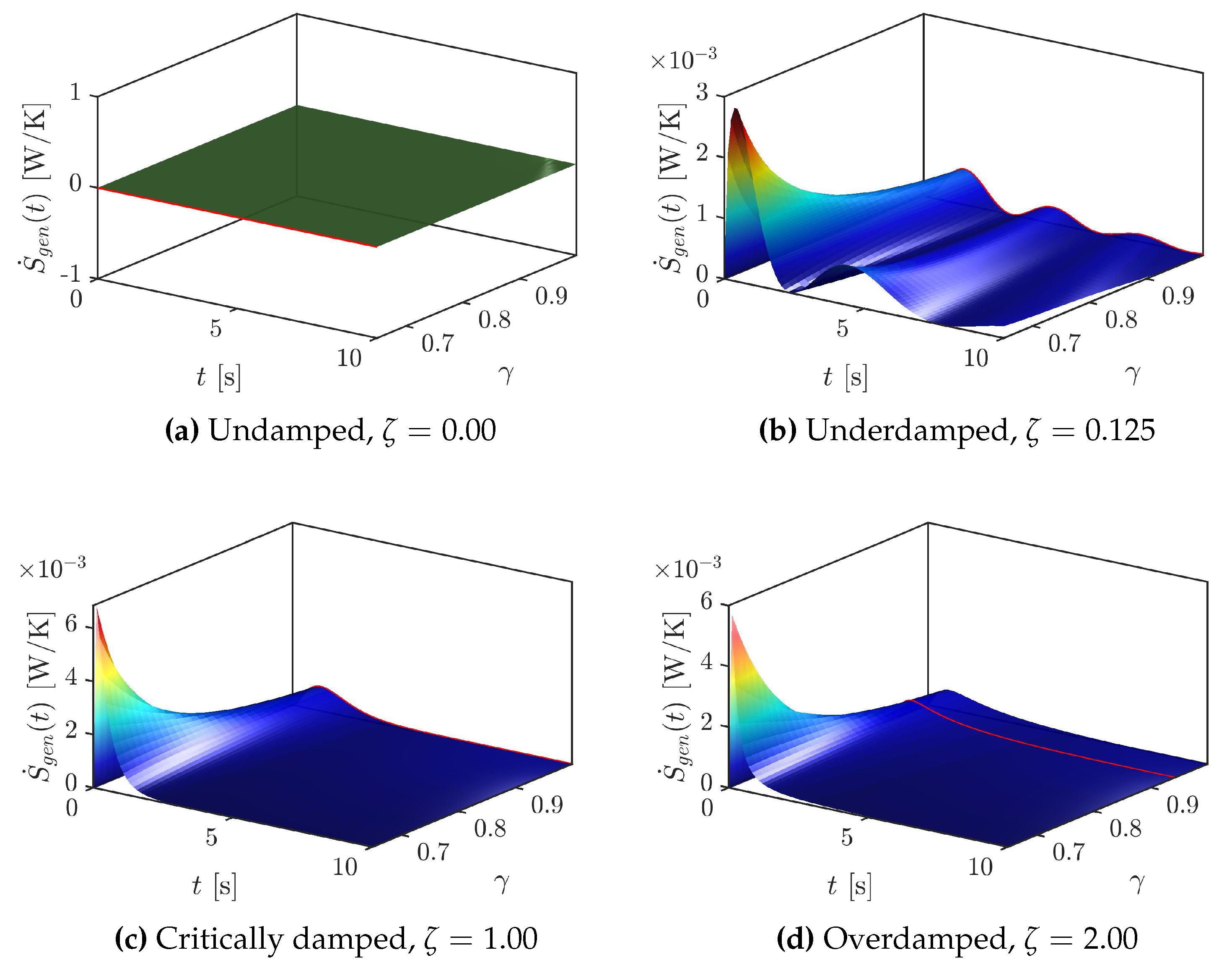
Subsequently, the entropy production of the MSD system was determined from its dynamic response under the conformable fractional sense. Hence, Figure 5 shows ${\dot{S}}_{gen}$ considering the four typical damping cases and varying the fractional order. In the first case, when $\zeta =0$ (undamped response), the entropy production is obviously zero; that is, the analyzed system becomes free-damped and reversible. When $\zeta =0.125$ (underdamped response), the entropy generation rate shows an initial overshoot, which decays with time and with the $\gamma$-powered variable coefficients of the model in Equation (13). Notice that the system presents a larger irreversible signature when $\gamma$ decreases, that is, the oscillations of ${\dot{S}}_{gen}$ increase, as expected from analyzing Figure 3. For the last two cases (critically and overdamped responses), the entropy production variation shows a greater overshoot, but it drops to zero faster than in the underdamped case. Furthermore, in all four cases plotted in Figure 5, the total entropy production $\Delta S_{gen}$ (J/K), which corresponds to the time integral of the entropy generation rate over the process, was determined. Results with the minimal value of $\Delta S_{gen}$ are presented as red curves in Figure 5 for illustrative purposes. Thus, the minimal $\Delta S_{gen}$ is found at $\gamma =1$ (the ordinary model) for $\zeta \le 1$, except when the system has an overdamped dynamics, where the minimal value is achieved at $\gamma <1$ (i.e., $\gamma =0.94$ minimizes $\Delta S_{gen}$ for $\zeta =2$). This means that if it is possible to reach a real dynamic response close to the conformable-based response in the overdamped case, the MSD system performs with the maximum efficiency.

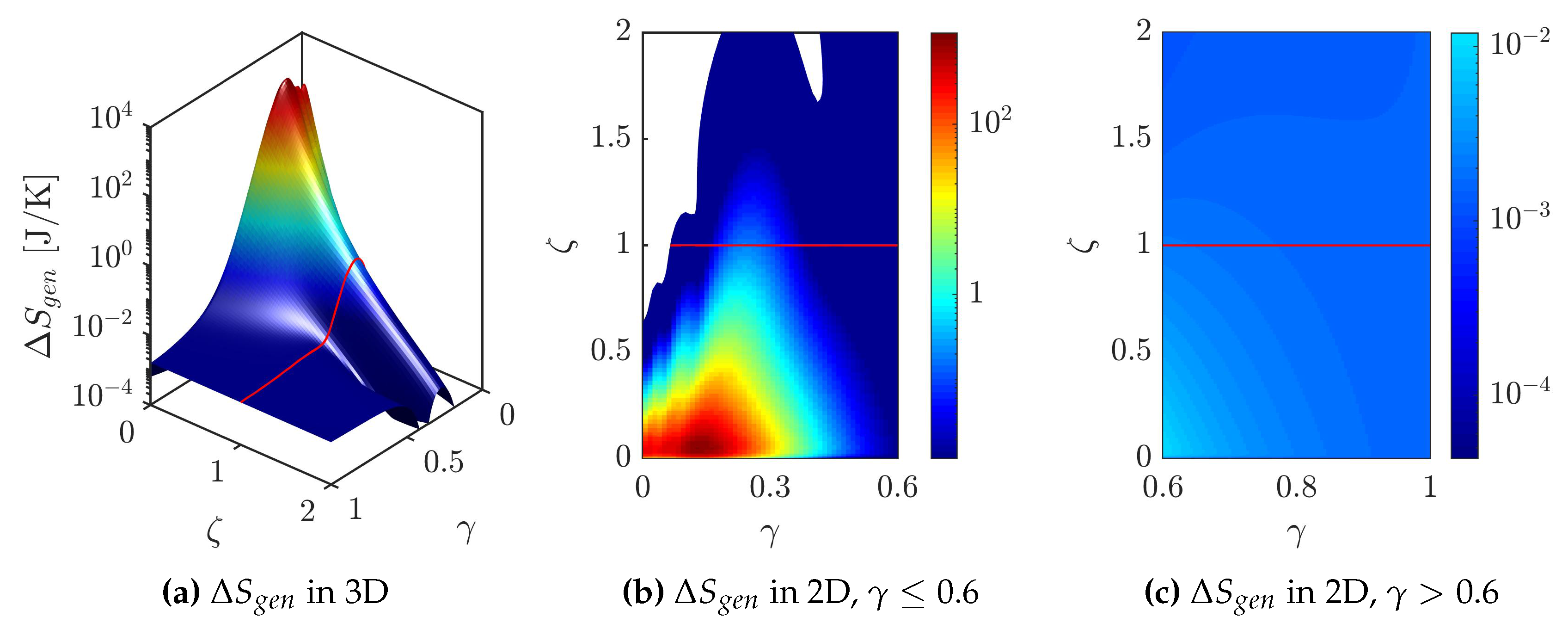
Figure 6 extends the information about the total entropy generated by varying the damping ratio and the fractional order. The effect of both $\zeta$ and $\gamma$ parameters on $\Delta S_{gen}$ is clear, which has a maximum value at $\zeta =0.04$ and $\gamma =0.13$ (cf. Figure 6a). Moreover, the white areas observed in Figure 6 correspond to values of $\Delta S_{gen}<{10}^{-4}$ J/K. In Figure 6b, it is also easy to recognize that the high and low entropy production regions are delimited by the critically damped case, when $\zeta =1$, and $\gamma <0.6$ (i.e., the higher and lower values of $\Delta S_{gen}$ can be reached with $\zeta <1$ and $\zeta >1$, respectively). Fortunately, these regions have no sense in this work, mainly due to the low conformable fractional order; however, they could be useful in other diverse specialized applications. Otherwise, Figure 6c shows the total entropy generation behavior for conformable fractional orders near the traditional order, which is interesting for most practical applications in different areas. Thence, $\Delta S_{gen}$ decreases when $\gamma$ and $\zeta$ increase, and it describes an apparent elliptic-parabolic shape until $\zeta$ is about 1.3. For damping ratios greater than 1.3, the conformable fractional orders $\gamma >0.6$ minimize $\Delta S_{gen}$, as shown in Figure 5d.

5. Conclusions

This work analyzed the entropy production and the dynamic response of a typical mass-spring-damper (MSD) system using the conformable fractional operator. Several simulations were carried out by varying the fractional order $\gamma$ and the damping ratio $\zeta$. They include the ordinary dynamic response when $\gamma =1$, and the typical damping cases (i.e., the underdamped, underdamped, critically damped and overdamped). Subsequently, the performance of the studied mechanical process was determined under the second law of thermodynamics, where entropy production represents a measurement of irreversibility. It was noticed that entropy production strongly depends on the fractional order $\gamma$ and the damping ratio $\zeta$. In general, the system process becomes less efficient (has a higher entropy production) when both $\gamma$ and $\zeta$ decrease; then, the settling time $t_s$ (s) increment as well. However, the minimal settling time was found equal to 3.54 s at $\zeta =0.78$ and $\gamma =1$ (the ordinary order); but it was proved that the ordinary order does not always render the minimal settling time. In the same fashion, considering the overdamped cases (i.e., $\zeta >1$), the minimal value of total entropy generation $\Delta S_{gen}$ is reached with a non-integer order $\gamma \in [0.6,1.0[$, whereas for the remaining cases, it is achieved with the ordinary order. The maximum value of $\Delta S_{gen}$ was determined at $\gamma =0.13$ and $\zeta =0.04$. Furthermore, when $\gamma >0.6$, the dynamic response is non-divergent and, $\Delta S_{gen}$ is at most ${10}^{-3}$ J/K. Otherwise, the response loses physical sense. It is worth mentioning that all results found here can be implemented in a real process with noisy or perturbed data, where the conformable model with $\gamma >0.6$ may describe its dynamic response better than the ordinary one. Moreover, as the entropy generation analysis principle dictates, any complex mechanical system can be subdivided into simple components, such as the studied MSD system here. Therefore, models and results presented in this work can be extended to a vast number of applications.

References

- Bai, W.; Dai, J.; Zhou, H.; Yang, Y.; Ning, X. Experimental and analytical studies on multiple tuned mass dampers for seismic protection of porcelain electrical equipment. Earthq. Eng. Eng. Vib. 2017, 16, 803–813. [Google Scholar] [CrossRef]
- Son, L.; Bur, M.; Rusli, M. A new concept for UAV landing gear shock vibration control using pre-straining spring momentum exchange impact damper. J. Vib. Control 2018, 24, 1455–1468. [Google Scholar] [CrossRef]
- Kim, S.M. Lumped element modeling of a flexible manipulator system. IEEE/ASME Trans. Mechatron. 2015, 20, 967–974. [Google Scholar] [CrossRef]
- Wang, D.; Mu, C. Adaptive-critic-based robust trajectory tracking of uncertain dynamics and its application to a spring–mass–damper system. IEEE Trans. Ind. Electron. 2017, 65, 654–663. [Google Scholar] [CrossRef]
- Derakhshandeh, J.F.; Arjomandi, M.; Cazzolato, B.S.; Dally, B. Harnessing hydro-kinetic energy from wake-induced vibration using virtual mass spring damper system. Ocean Eng. 2015, 108, 115–128. [Google Scholar] [CrossRef]
- Takeya, K.; Sasaki, E.; Kobayashi, Y. Design and parametric study on energy harvesting from bridge vibration using tuned dual-mass damper systems. J. Sound Vib. 2016, 361, 50–65. [Google Scholar] [CrossRef]
- Baleanu, D.; Guvenc, Z.B.; Machado, J.T. (Eds.) New Trends in Nanotechnology and Fractional Calculus Applications; Springer: Berlin/Heidelberg, Germany, 2010. [Google Scholar]
- De Oliveira, E.C.; Tenreiro Machado, J.A. A review of definitions for fractional derivatives and integral. Math. Prob. Eng. 2014, 2014, 238459. [Google Scholar] [CrossRef] [Green Version]
- Machado, J.T.; Mainardi, F.; Kiryakova, V. Fractional calculus: Quo vadimus? (Where are we going?). Fract. Calc. Appl. Anal. 2015, 18, 495–526. [Google Scholar]
- Duarte Ortigueira, M. Fractional Calculus for Scientists and Engineers; Springer: Berlin, Germany, 2011. [Google Scholar]
- Uchaikin, V.V. Fractional Derivatives for Physicists and Engineers; Springer: Berlin, Germany, 2013; Volume 2. [Google Scholar]
- Caputo, M.; Fabrizio, M. A new definition of fractional derivative without singular kernel. Progr. Fract. Differ. Appl. 2015, 1, 1–13. [Google Scholar]
- Atangana, A.; Baleanu, D. New fractional derivatives with non-local and non-singular kernel: Theory and application to heat transfer model. Therm. Sci. 2016, 20, 763–769. [Google Scholar]
- Khalil, R.; Al Horani, M.; Yousef, A.; Sababheh, M. A new definition of fractional derivative. J. Comput. Appl. Math. 2014, 264, 65–70. [Google Scholar] [CrossRef]
- Abdeljawad, T. On conformable fractional calculus. J. Comput. Appl. Math. 2015, 279, 57–66. [Google Scholar] [CrossRef]
- Genesiz, Y.; Baleanu, D.; Kurt, A.; Tasbozan, O.C. New exact solutions of Burgers’ type equations with conformable derivative. Waves Random Complex Media 2017, 27, 103–116. [Google Scholar] [CrossRef]
- Morales-Delgado, V.; Gómez-Aguilar, J.; Taneco-Hernández, M. Analytical solutions of electrical circuits described by fractional conformable derivatives in Liouville-Caputo sense. Int. J. Electron. Commun. 2018, 85, 108–117. [Google Scholar] [CrossRef]
- Ertik, H.; Calik, A.E.; Sirin, H.; Sien, M.; Oder, B. Investigation of electrical RC circuit within the framework of fractional calculus. Rev. Mex. Fis. 2015, 61, 58–63. [Google Scholar]
- Abdeljawad, T.; Al-Horani, M.; Khalil, R. Conformable fractional semigroups of operators. J. Semigroup Theory Appl. 2015, 7, 1–9. [Google Scholar]
- Ortega, A.; Rosales, J.J.; Martínez, L.; Cruz-Duarte, J.M. Analysis of projectile motion in view of conformable derivative. Open Phys. 2018, 16, 581–587. [Google Scholar]
- Carreño, C.A.; Rosales, J.J.; Merchán, L.R.; Lozano, J.M.; Godínez, F.A. Comparative analysis to determine the accuracy of fractional derivatives in modeling supercapacitors. Int. J. Circuit Theory Appl. 2019, 47, 1603–1614. [Google Scholar] [CrossRef]
- Rosales, J.J.; Godínez, F.A.; Banda, V.V.; Valencia, G.H. Analysis of the Drude model in view of the conformable derivative. Optik 2019, 178, 1010–1015. [Google Scholar] [CrossRef]
- Ortigueira, M.D.; Tenreiro Machado, J.A. What is a fractional derivative? J. Comput. Phys. 2015, 293, 4–13. [Google Scholar] [CrossRef]
- Zhao, D.; Li, T. On conformable delta fractional calculus on time scales. J. Math. Comput. 2016, 16, 324–335. [Google Scholar] [CrossRef] [Green Version]
- Zhao, D.; Luo, M. General conformable fractional derivative and its physical interpretation. Calcolo 2017, 54, 903–917. [Google Scholar] [CrossRef]
- Tarasov, V.E. No nonlocality. No fractional derivative. Commun. Nonlinear Sci. Numerical Simul. 2018, 62, 157–163. [Google Scholar] [CrossRef] [Green Version]
- Achar, B.N.; Hanneken, J.W.; Enck, T.; Clarke, T. Dynamics of the fractional oscillator. Phys. A Stat. Mech. Its Appl. 2001, 297, 361–367. [Google Scholar] [CrossRef]
- Achar, B.N.; Hanneken, J.W.; Enck, T.; Clarke, T. Response characteristics of a fractional oscillator. Phys. A Stat. Mech. Its Appl. 2002, 309, 275–288. [Google Scholar] [CrossRef]
- Achar, B.N.; Hanneken, J.W.; Enck, T.; Clarke, T. Damping characteristics of a fractional oscillator. Phys. A Stat. Mech. Its Appl. 2004, 339, 311–319. [Google Scholar] [CrossRef]
- Berman, M.; Cerderbaum, L. Fractional driven-damped oscillator and its general closed form exact solution. Phys. A Stat. Mech. Its Appl. 2018, 505, 744–762. [Google Scholar] [CrossRef]
- Bejan, A. Entropy generation minimization: The new thermodynamics of finite-size devices and finite-time processes. J. Appl. Phys. 1996, 79, 1191–1218. [Google Scholar] [CrossRef] [Green Version]
- Bejan, A. Entropy generation minimization, exergy analysis, and the constructal law. Arab. J. Sci. Eng. 2013, 38, 329–340. [Google Scholar] [CrossRef]
- Sciacovelli, A.; Verda, V.; Sciubba, E. Entropy generation analysis as a design tool—A review. Renew. Sustain. Energy Rev. 2015, 43, 1167–1181. [Google Scholar] [CrossRef]
- Sunar, M.; Sahin, A.Z.; Yilbas, B.S. Entropy generation rate in a mechanical system subjected to a damped oscillation. Int. Exergy 2015, 17, 401–411. [Google Scholar] [CrossRef]
- Rosales, J.; Gómez, J.F.; Guía, M.; Tkach, V. Fractional electromagnetic waves. In Proceedings of the 11th International Conference Laser and Fiber-Optical Networks Modeling, Kharkov, Ukraine, 5–8 September 2011. [Google Scholar]
- Atangana, A.; Baleanu, D.; Alsaedi, A. New properties of conformable derivative. Open Math. 2015, 13, 889–898. [Google Scholar] [CrossRef]
- Gómez-Aguilar, J.F.; Rosales-García, J.J.; Bernal-Alvarado, J.J.; Córdova-Fraga, T.; Guzmán-Cabrera, R. Fractional mechanical oscillators. Rev. Mex. Física 2012, 58, 348–352. [Google Scholar]
- Gómez, F.; Rosales, J.; Guía, M. RLC electrical circuit of non-integer order. Cent. Eur. Phys. 2013, 11, 1361–1365. [Google Scholar] [CrossRef] [Green Version]
- Gómez-Aguilar, J.; Morales-Delgado, V.; Taneco- Hernández, M.; Baleanu, D.; Escobar-Jiménez, R.; Al Qurashi, M. Analytical solutions of the electrical RLC circuit via Liouville–Caputo operators with local and non-local kernels. Entropy 2016, 18, 402. [Google Scholar] [CrossRef]
- Ebaid, A.; Masaedeh, B.; El-Zahar, E. A new fractional model for the falling body problem. Chin. Phys. Lett. 2017, 34, 020201:1-3. [Google Scholar] [CrossRef]
Figure 1.
Sketch of the studied simple mass-spring-damper (MSD) system.
Figure 2.
Displacement of the MSD system using the conformable model, considering the four typical damping cases and varying the fractional order .
Figure 3.
Phase planes vs. of the MSD system using the conformable model, considering the four typical damping cases and varying the fractional order .
Figure 4.
Settling time (s) of the MSD system using the conformable model, determined by varying the fractional order and the damping ratio .
Figure 5.
Entropy generation rate of the MSD system using the conformable model, considering the four typical damping cases and varying the fractional order .
Figure 6.
Total entropy generation (J/K) of the MSD system using the conformable model, varying the damping ratio and the fractional order .
© 2020 by the authors. Licensee MDPI, Basel, Switzerland. This article is an open access article distributed under the terms and conditions of the Creative Commons Attribution (CC BY) license (http://creativecommons.org/licenses/by/4.0/).
Share and Cite
MDPI and ACS Style
Cruz-Duarte, J.M.; Rosales-García, J.J.; Correa-Cely, C.R. Entropy Generation in a Mass-Spring-Damper System Using a Conformable Model. Symmetry 2020, 12, 395. https://0-doi-org.brum.beds.ac.uk/10.3390/sym12030395
AMA Style
Cruz-Duarte JM, Rosales-García JJ, Correa-Cely CR. Entropy Generation in a Mass-Spring-Damper System Using a Conformable Model. Symmetry. 2020; 12(3):395. https://0-doi-org.brum.beds.ac.uk/10.3390/sym12030395
Chicago/Turabian StyleCruz-Duarte, Jorge M., J. Juan Rosales-García, and C. Rodrigo Correa-Cely. 2020. "Entropy Generation in a Mass-Spring-Damper System Using a Conformable Model" Symmetry 12, no. 3: 395. https://0-doi-org.brum.beds.ac.uk/10.3390/sym12030395
Note that from the first issue of 2016, this journal uses article numbers instead of page numbers. See further details here.