Representing Measurement as a Thermodynamic Symmetry Breaking

Abstract

Descriptions of measurement typically neglect the observations required to identify the apparatus employed to either prepare or register the final state of the “system of interest.” Here, we employ category-theoretic methods, particularly the theory of classifiers, to characterize the full interaction between observer and world in terms of information and resource flows. Allocating a subset of the received bits to system identification imposes two separability constraints and hence breaks two symmetries: first, between observational outcomes held constant and those allowed to vary; and, second, between observational outcomes regarded as “informative” and those relegated to purely thermodynamic functions of free-energy acquisition and waste heat dissipation. We show that breaking these symmetries induces decoherence, contextuality, and measurement-associated disturbance of the system of interest.

1. Introduction

Measurements of macroscopic systems—indeed, any observations made in any setting, however informal—pose a problem in quantum theory because they appear to violate the theory’s fundamental symmetry: unitarity or conservation of information (see [1,2] for comprehensive reviews). Irreversibly recordable observational outcomes are, in particular, classical by definition, as emphasized by Bohr [3] and many others. Obtaining such classical outcomes, however, requires physically interacting with the world. What is the relationship between the classical outcomes that observers obtain and the physical interactions via which they obtain them? To investigate this question, we turn to a relatively-neglected aspect of measurement: the identification, by the observer, of the physical system being observed. We are interested, in particular, in how an observer identifies macroscopic systems such as laboratory apparatus.

The ability of observers to identify macroscopic systems is generally taken for granted even when discussing systems with explicitly quantum properties (see [4] for a recent review). Schrödinger, for example, had no problem identifying the steel chamber containing his cat, although it contains, and may well itself be a component of, a quantum system in an entangled state [5]. More tellingly, Wigner had no trouble identifying and conversing with his friend, although his friend is by assumption a component of a quantum system in an entangled state, the other component of which may be as large as an entire laboratory [6]. When performing a Bell/EPR experiment, Alice and Bob similarly have no trouble identifying and reading their respective apparatus pointers, although these pointers are components of a spacelike-extended quantum system in an entangled state [7]. Appeals to system–environment decoherence [8,9,10] or state broadcasting [11,12,13,14] contribute nothing to understanding the ability of observers to identify such macroscopic systems, as they assume a priori a fixed and known (in the case of state broadcasting, by multiple observers) system–environment boundary [15,16,17]. Modifying quantum theory by introducing a physical “collapse” mechanism and hence an “ontic” classical realm at large scales (e.g., [18,19,20]) similarly does not help, as the system-identification problem also arises, and arises for the same reasons, in a classical setting [17].

A second common assumption of descriptions of measurement, whether quantum or classical, is that observers are supplied with whatever free energy they require to make and record their observations, including the observations used to identify the system(s) of interest, by mechanisms that are entirely independent of the systems or processes being observed. The thermodynamic sinks into which observers dump waste heat are similarly assumed to be independent of the systems or processes being observed. These assumptions render the “unobserved environment” more than just a resource for decoherence; this environment, or some larger system of which it a component, must also supply free energy and dissipate heat, and do both in ways that do not disturb the observations.

Quantum theory provides a formal description of the interaction between two systems that assumes nothing about the structures or properties of the systems beyond the representation of their states spaces by Hilbert spaces. Here, we study the physics of system identification by observers within a nonrelativistic quantum-theoretic framework making only two additional assumptions:

Assumption 1

(Separability). We assume a decomposition of $U=$ “everything” into $OW$, where O is the “observer” and W is the “world” with which the observer interacts. We require that the state $|U\rangle$ be separable as $|U\rangle =|OW\rangle =|O\rangle |W\rangle$, at least up to some recoherence time that is long with respect to any time interval of interest.

Assumption 2

(Finiteness). We assume the Hilbert space ${\mathcal{H}}_U={\mathcal{H}}_O\otimes {\mathcal{H}}_W$ has finite dimension $d_U=d_O+d_W$.

Assumption 1 is required for the idea of observation to make sense: the observer O can only irreversibly change state after an observation, i.e., can only record an observation, if $|O\rangle$ is well-defined, and the world W can only have an observable state if $|W\rangle$ is well-defined. Assumption 2 is required for any physically-realistic observer O interacting with any finite local (i.e., “observable”) world W.

With these assumptions, we can write a Hamiltonian:

$$H_U=H_O+H_W+H_{OW},$$

(1)

where $H_{OW}$ is the $O-W$ interaction, and can choose bases for O and W such that, with respect to a time parameter t characterizing U:

$$H_{OW}(t)={\beta }^k{k}_B{T}^k\sum _i{\alpha }_i^k(t)M_i^k,$$

(2)

where $k=O$ or W, $i=1\dots N$ for finite N, the ${\alpha }_i^k(t)$ are real functions with codomains $[0,1]$ such that:

$$\sum _i{\int }_{\mathsf{\Delta }t}dt{\alpha }_i^k(t)=\mathsf{\Delta }t$$

(3)

for every finite $\mathsf{\Delta }t$, $k_B$ is Boltzmann’s constant, $T^k$ is k’s temperature, ${\beta }^k\ge$ ln 2 is an inverse measure of k’s average per-bit thermodynamic efficiency that depends on the internal dynamics $H_k$, and the $M_i^k$ are Hermitian operators with binary eigenvalues representing “questions to Nature” with yes–no answers [21]. Here, O and W are each regarded as “observing” the other; the operators $M_i^O$ act on W, while the operators $M_i^W$ act on O. To assure that O and W are “interesting” from the point of view system identification, we assume that the sets $\left\{M_i^k\right\}$ of operators are large enough that, for any $M_i^k$, there is at least one $M_j^k$ such that $[M_i^k,M_j^k]=0$ and at least one $M_l^k$ such that $[M_i^k,M_l^k]\ne 0$. The latter requirement enables violation of the Leggett–Garg inequality [22] or, equivalently, Kochen–Specker contextuality [23]. Hence, $H_{OW}$ is manifestly a quantum interaction. However, as noted above, Equations (2) and (3) make no reference to either $H_O$ or $H_W$, and are indeed independent of any assumptions about the purity or separability of the states $|O\rangle$ or $|W\rangle$, the decomposition of either O or W into subsystems, or the interactions, if any, between such subsystems.

The idea that nature “answers” an observer’s questions is classical, and implies an irreversible state change [24]: each question from O that W “answers” transfers one bit from W to O and is paid for by the transfer of ${\beta }^O{k}_B{T}^O$ from O to W. This situation is completely symmetric: each question from W that O “answers” transfers one bit from O to W and is paid for by the transfer of ${\beta }^W{k}_B{T}^W$ from W to O. Given Equation (3), the action required for k to transfer N bits in time $\mathsf{\Delta }t$ is:

$${\int }_{\mathsf{\Delta }t}dt(ı\hslash )\ln \mathcal{P}(t)=N{\beta }^k{k}_B{T}^k\mathsf{\Delta }t$$

(4)

where $\mathcal{P}(t)=exp(-(ı/\hslash )H_{OW}t)$. Informational symmetry clearly requires ${\beta }^O{T}^O={\beta }^W{T}^W$ during any finite $\mathsf{\Delta }t$.

The representation of observation given by Equations (2)–(4) simply describes an exchange of energy for information. How then is identifying the system of interest distinguished, physically, from measuring its state? The answer, we suggest, lies in two asymmetries: the asymmetry between bits representing the “system of interest” and bits representing the “apparatus” and the asymmetry between bits that are processed as “information about W” and bits that are processed as fuel, i.e., as free energy to drive the processing of the bits considered informative, or as waste heat. These asymmetries are imposed not by $H_{OW}$ but rather by the structure of $H_O$ (or, if viewing W as an observer, by $H_W$); hence, they are features of the information-processing architecture of O (or W). In what follows, we make this suggestion precise as follows:

• We rigorously define a “system” contained within W, relative to O’s observational capabilities, by employing the natural equivalence between binary-valued observables and binary classifiers as defined [25] and the category-theoretic construction of a cocone (for review, see [26]).
• We formulate the distinction between system identification and pointer-state measurement as a collection of equivalence relations on cocones, and showing that: (1) transitions between cocone equivalence classes can be represented more generally as groupoid operations; and (2) these groupoid operations correspond to entanglement swaps that result in O-relative decoherence [27].
• We show that such entanglement swaps can also be viewed as a context switches as defined [28,29,30] and hence that Born-rule probability distributions over measurement outcomes are generically context-dependent, i.e., generically display Kochen–Specker contextuality.
• We show that free-energy acquisition and waste-heat dissipation into the “environment” component of W can generically have non-negligible effects on observational outcomes due to entanglement swapping/contextuality.

We begin in Section 2 by providing a fully sequential model of interaction as (mutual) measurement, and then coarse-graining time to generalize this sequential model. We then show that, for finite U, the assumption of separability is equivalent to the assumption that O and W communicate by classical communication, i.e., exchange of fungible [31] bit strings, via an ancillary, noise-free classical channel. We provide a formal description of system identification in Section 3, showing that any “system of interest” must have distinct reference and pointer components, that these components can be represented as cocones over distinct sets of observables related by a predictability sieve [9], and that distinguishing these components induces both component-scale decoherence and system-scale contextuality. We then show in Section 4 that, if system identification is held fixed, system state is generically vulnerable to disturbance as free energy is extracted from and heat is dissipated into the environment. We conclude in Section 5 by briefly discussing the implications of these results for the architectures of “information gathering and using systems” (IGUSs, i.e., observers [32]) and the relationship between decoherence and temporal coarse-graining.

2. Interaction as Mutual Measurement by $\mathit{O}$ and $\mathit{W}$

2.1. Sequential Measurements

The simplest physical interactions, and hence the simplest measurements, are sequential: O selects and deploys one operator $M_i^O$ during each interval $\mathsf{\Delta }t$, receiving in consequence one bit of information from and transferring ${\beta }^O{k}_B{T}^O$ of heat to W. The interaction has the same description from W’s perspective, only replacing superscripts O with W.

Following [17], sequential measurements can be represented by choosing the functions ${\alpha }_i^k(t)$ to be rectangular functions, but replacing the typical fixed duty cycle n with variable duty cycles $n_i^k(t)$ “chosen” by k, i.e., determined by the unspecified internal dynamics $H_k$:

$${\Pi }_i^{k(s,m)}(t)=\sum _{j=0}^{m-1}\Pi (t-(n_i^k(t)j+s+1/2)\mathsf{\Delta }t)$$

(5)

where the offset $s,0\le s\le n(0)-1$ determines when $M_i^k$ is first deployed, m is the total (finite but unlimited) number of times $M_i^k$ is deployed, and:

$$\Pi (t)=\left\{\begin{array}{cc}\hfill 0& \mathrm{if}\left|t\right|>1/2;\hfill \\ \hfill 1/2& \mathrm{if}\left|t\right|=1/2;\hfill \\ \hfill 1& \mathrm{if}\left|t\right|<1/2.\hfill \end{array}\right.$$

Each ${\Pi }^{(i,m)}(t)$ is a sequence, starting at $t=s$, of m unit-height rectangular pulses with width $\mathsf{\Delta }t$, with separation given by $n_i^k(t)\mathsf{\Delta }t$. In this case, we have:

$$H_{OW}(t)={\beta }^k{k}_B{T}^k\sum _i{\Pi }_i^{k(s,m)}(t)M_i^k$$

(6)

with action still given by Equation (4).

The quantization of both action and information guarantees that time can always be fine-grained sufficiently to render measurements sequential. It is convenient in the followings, however, to coarse-grain time and view some measurements as carried out simultaneously (or “in parallel”). Clearly, this is only possible for subsets of mutually-commuting measurement operators. In what follows, we abuse the notation by employing $M_k^P$ to indicate either the kth individual operator as above or the kth subset of mutually-commuting operators where the ambiguity presents no problems, and the notation ${\left\{M^P\right\}}_k$ for the kth subset of mutually-commuting operators where more explicitness is called for. We reserve $\mathsf{\Delta }t$ to indicate the interval required to deploy one operator and obtain one bit as above and use $\tau$ to indicate an integer multiple of this interval during which a mutually-commuting subset of operators is deployed and multiple bits are obtained.

2.2. Mutual Measurement Is Classical Communication

We can, as is now standard, think of O and W as communicating agents, i.e., we can think of $H_{OW}$ as specifying a communication channel.

Theorem 1.

With $H_{OW}$ given by Equation (2), the specified communication channel is classical, ancillary, and free from classical noise.

Proof of Theorem 1.

No generality is lost by regarding the interaction $H_{OW}$ as specifying a strictly sequential deployment of the $M_i^k$ as in Equation (6). In this case, the action in Equation (4) transfers one bit, corresponding to one of the two eigenvalues of the deployed operator $M_i^O$, from W to O during each interval $\mathsf{\Delta }t$, and one bit, corresponding to one of the two eigenvalues of the deployed operator $M_j^W$, from O to W during this same $\mathsf{\Delta }t$. This sequential exchange of bits constitutes classical communication. There are no physical degrees of freedom other than those of O and W, thus the communication channel is ancillary and free from classical noise.  □

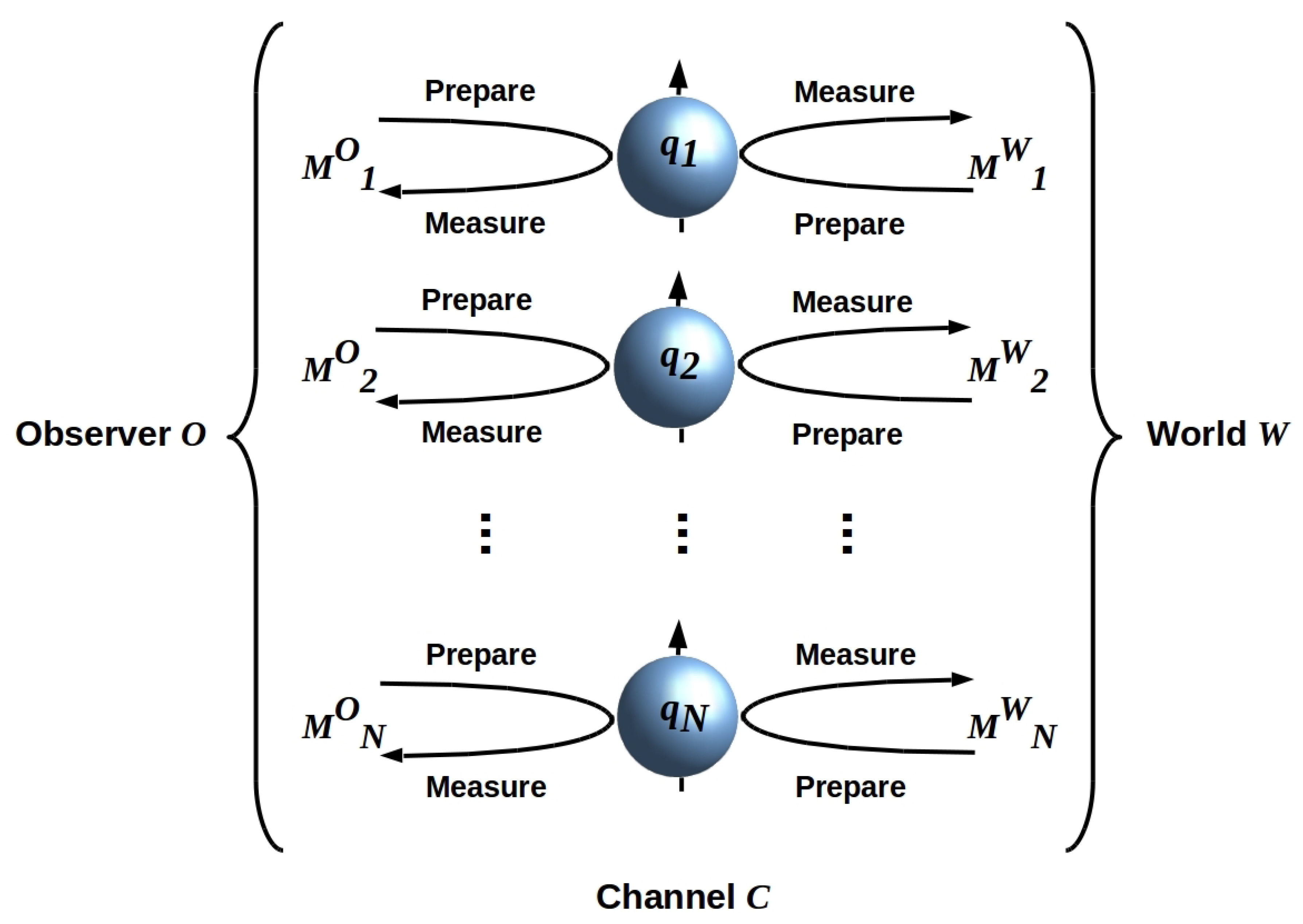
While the exchange of bits between O and W is free of classical noise, the $O-W$ channel flips each bit, independently, with finite probability unless O and W are assumed to share a quantum reference frame a priori [33], i.e., only if O and W share a basis. We assume such a shared basis for simplicity. As an explicit example, suppose O and W alternate preparation and measurement of an array of non-interacting qubits, as shown in Figure 1. Assuming a shared reference frame for $s_z$ preparations and measurements, the encoded bit values are preserved in either direction.

It is important to emphasize that while by Theorem 1 $H_{OW}$ can be considered to define a classical communication channel, $H_{OW}$ is, as noted above, a manifestly quantum interaction that can violate the Leggett–Garg inequality and display Kochen–Specker contextuality, as discussed in detail in Section 3.5 below. It is also important to emphasize that, while the bits received by O provide a representation, for O, of the state $|W\rangle$, they do not, by themselves, provide any information to O about the decompositional structure of W, if any, and do not specify the internal Hamiltonian $H_W$. This is a simple consequence of linearity: we are free to choose any decomposition $W=SE$ and write ${\mathcal{H}}_W={\mathcal{H}}_S\otimes {\mathcal{H}}_E$ and $H_W=H_S+H_E+H_{SE}$ without affecting the interaction $H_{OW}$ and hence O’s observational outcomes in any way. We need, therefore, make no assumptions about the “ontic” state of W as noted above; whether this state is separable or pure makes no difference to O’s observational outcomes. What is of interest in what follows is solely the “epistemic” state of W for O; the notation “$|W\rangle$” is henceforward used strictly to denote this “epistemic” state. As above, the same considerations apply to the representation of $|O\rangle$ by W.

3. System Identification and Measurement by $\mathit{O}$

3.1. Systems Require Reference Components with Invariant States

Identifying a system S in W requires distinguishing it from the rest of W, which we call the “environment” E of S. In order for this S to have a measurable state $|S\rangle$, $|W\rangle$ must be separable as $|W\rangle =|SE\rangle =|S\rangle |E\rangle$. Here, the recognition that $|W\rangle$, and hence also $|S\rangle$ and $|E\rangle$, are “epistemic” states, i.e., states for O, is consistent with the general observer-relativity of separability [34,35,36,37].

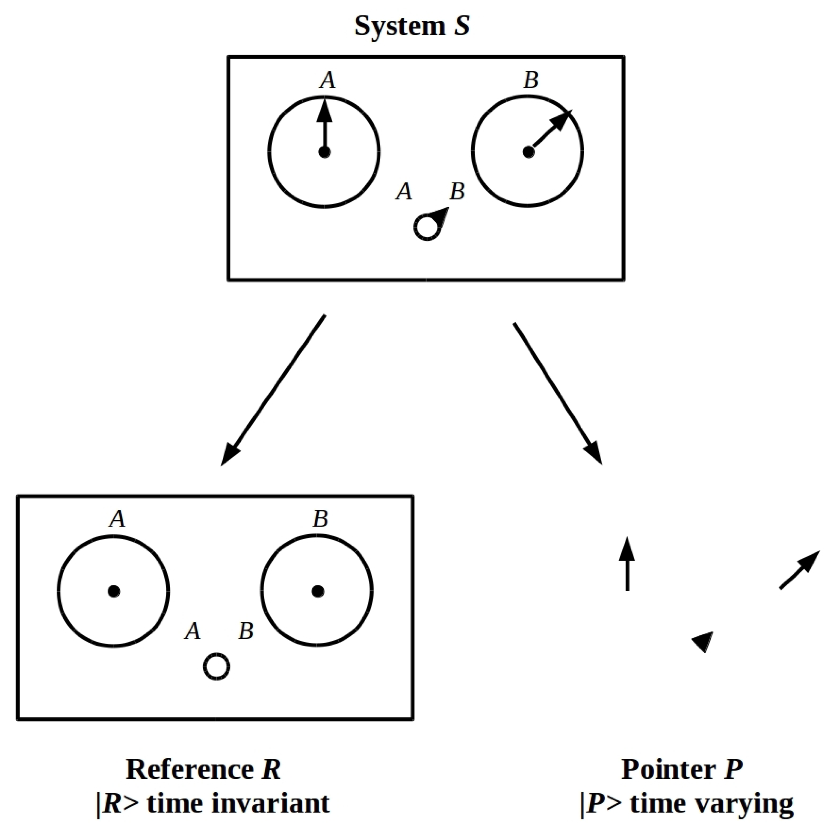
The system S having a measurable state is, however, not yet sufficient for S to be identifiable by O. In addition, S must have some component, which we call the “reference” R, that has a time invariant, and hence reliably recognizable state. We must, therefore, be able to write $S=RP$, where P is the usual “pointer” component of S, and require (O-relative) separability $|S\rangle =|RP\rangle =|R\rangle |P\rangle$, where $|R\rangle$ is a time-invariant “reference state” used for system identification and $|P\rangle$ is the usual time-varying “pointer state” that is of interest to O. This decomposition into R and P is illustrated in Figure 2. Any identifiable macroscopic object, e.g., any item of laboratory apparatus, clearly must support such a decomposition.

The decompositions $W=SE$ and $S=RP$ induce partitions of the set $\left\{M_i^O\right\}$ of operators with which O interacts with W; suppressing redundant superscripts, we will write $\left\{M_i^O\right\}=\left\{M_j^R\right\}\cup \left\{M_k^P\right\}\cup \left\{M_l^E\right\}$ where all unions are disjoint. We will also write $H_{OW}=H_{OR}+H_{OP}+H_{OE}$, where $H_{OR}$ implements system identification, $H_{OP}$ implements pointer-state measurement, and $H_{OE}$ implements free-energy acquisition and waste-heat dissipation. Each of these interactions can, by Theorem 1, be regarded as classical bit exchange. We write numbers of exchanged bits as $N=N^R+N^P+N^E$ and inverse thermodynamic efficiencies as $N{\beta }^O=N^R{\beta }^R+N^P{\beta }^P+N^E{\beta }^E$ with the restriction ${\beta }^R,{\beta }^P,{\beta }^E\ge$ ln 2. As shown in Section 4 below, it is inequalities among the ${\beta }^R,{\beta }^P$, and ${\beta }^E$ that break the thermodynamic symmetry of $H_{OW}$. Without such symmetry breaking, R and P cannot be distinguished from E, thus neither system identification nor pointer measurement can occur.

For S to remain identifiable over multiple rounds of measurement, the $M_j^R$ must satisfy the commutation and predictability sieve [9] requirements:

$$\forall j,k,[M_j^R,M_k^R]=0;\forall j,[M_j^R,H_{O}W]=0.$$

(7)

In general, neither the $M_k^P$ nor the $M_l^E$ will all commute. Failure of commutativity among the $M_k^P$ is exemplified by apparatus calibration procedures [17], failure of commutativity among the $M_l^E$ by such events as laboratory power failures.

3.2. Reference Components Can Be Represented as Cocones over One-Bit Classifiers

As emphasized above, system identification must be implemented by the internal process executed by the observer, i.e., by the Hamiltonian $H_O$. Indeed, it can only be $H_O$ that assigns different functions to the inputs provided by $H_{OW}$, and hence decomposes $H_{OW}$ into component system identification, measurement, and energy–management interactions. While it is now commonplace to regard observers as Bayesian agents [38,39] and a handful of architectural models of observers have been proposed [32,40,41,42], the question of generic requirements on $H_O$ to implement “observation” in any meaningful sense has been largely neglected. We approach this question here using tools and methods from the theory of formal languages and category theory. These allow us to specify a minimal virtual machine [43] that must be implemented by $H_O$ in any O capable of both identifying and measuring the pointer states of an external system. This approach is independent of the physical implementation of $H_O$, up to requiring that O has sufficient degrees of freedom. We can, without loss of generality, view O as implemented by a suitable circuit of quantum gates [44].

Barwise and Seligman [25] introduced the idea of a “classifier” as implementing the relation between “tokens” in some language and the “types” to which they belong. We first characterize this notion formally, and then show that the one-bit measurement operators $M_i^O$ can be identified with one-bit classifiers. Mathematical operations on classifiers become, in this case, formal specifications of computations on measurement outcomes implemented by $H_O$.

Definition 1.

A classifier $\mathcal{A}$ is a triple $<Tok(\mathcal{A}),Typ(\mathcal{A}),{\vDash }_{\mathcal{A}}>$ where $Tok(\mathcal{A})$ is a set of “tokens”, $Typ(\mathcal{A})$ is a set of “types”, and ${\vDash }_{\mathcal{A}}$ is a “classification” relation between tokens and types.

A classifier for voltmeters, for example, would assign all examples (i.e., tokens) of voltmeters to the general class (i.e., type) “voltmeters”; similarly a classifier for observations (tokens) of some particular voltmeter V would assign all such observations, but no observations of other systems, including other voltmeters, to the class (type) “observations of V” (see [26] for extensive review with examples, and [45] for a specific application to system identification). The simplest classifiers implement one-bit, yes–no classification decisions, i.e., they group entities (tokens) having some property $\mathcal{P}$ into classes (types) “entities with property $\mathcal{P}$”; for example, a one-bit classifier for black objects would group all such objects, excluding all objects that were not black.

A natural map between classifiers is the “infomorphism” [25] defined as follows:

Definition 2.

Given two classifiers $\mathcal{A}=<Tok(\mathcal{A}),Typ(\mathcal{A}),{\vDash }_{\mathcal{A}}>$ and $\mathcal{B}=<Tok(\mathcal{B}),Typ(\mathcal{B}),{\vDash }_{\mathcal{B}}>$, an infomorphism $f:\mathcal{A}\to \mathcal{B}$ is a pair of maps $\overrightarrow{f}:Tok(\mathcal{B})\to Tok(\mathcal{A})$ and $\overleftarrow{f}:Typ(\mathcal{A})\to Typ(\mathcal{B})$ such that $\forall b\in Tok(\mathcal{B})$ and $\forall a\in Typ(\mathcal{A})$, $\overrightarrow{f}(b){\vDash }_{\mathcal{A}}a$ if and only if $b{\vDash }_{\mathcal{B}}\overleftarrow{f}(a)$.

Intuitively, an infomorphism “transmits the information” from one classifier to another, so that, e.g., “b is type B” can encode or represent the information “a is type A”. “Information” here is not simply a quantity of bits (“Shannon information”), but is rather the set of logical constraints imposed by Definition 2; hence, it is “pragmatic information” as defined [46]. This idea of transmitting information motivates the definition of an “information channel” [25], itself a classifier, expressed as a collection $\{g_i:{\mathcal{A}}_i\to \mathcal{C}\}$ of infomorphisms with a common codomain, or “core” $\mathcal{C}$. Here, the classifier $\mathcal{C}$ encodes or represents the information (i.e., the logical constraints) encoded jointly by the ${\mathcal{A}}_i$; alternatively, $\mathcal{C}$ can be thought of as a shared memory jointly accessed by the ${\mathcal{A}}_i$. The sense which channels encode sets of mutual constraints holding between classifiers is further elaborated in [25,26] where the notion of a classifier is extended to that of a “local logic” by specifying a subset (possibly a singlet) of tokens satisfying all of the types, and the notion of an infomorphism is extended to a “logic infomorphism” that preserves this additional structure. It is natural to think of a local logic as “identifying” the token(s) that satisfy all of its types, logic infomorphisms transferring token-identification information between local logics, and channels comprising sets of logic infomorphisms as encoding mutual constraints that assemble multiple identified tokens—which can naturally be thought of as “parts” [45]—into a larger identified system.

Given suitable commutativity conditions, a collection of channels $\{g_{ij}:{\mathcal{A}}_{ij}\to {\mathcal{C}}_j\}$ admits a colimit, a single channel $\mathbf{C}$ that collects all of the classification information encoded by the ${\mathcal{A}}_{ij}$. The conditions are:

• The ${\mathcal{A}}_{ij}$ must be representable as a finite nonredundant set $\left\{{\mathcal{A}}_k\right\}$ with infomorphisms $fij:{\mathcal{A}}_i\to {\mathcal{A}}_j$.
• There exist infomorphisms $h_i:{\mathcal{C}}_i\to \mathbf{C}$ and $h_{ij}:{\mathcal{C}}_i\to {\mathcal{C}}_j$.
• All compositions of infomorphisms with codomain $\mathbf{C}$ commute.

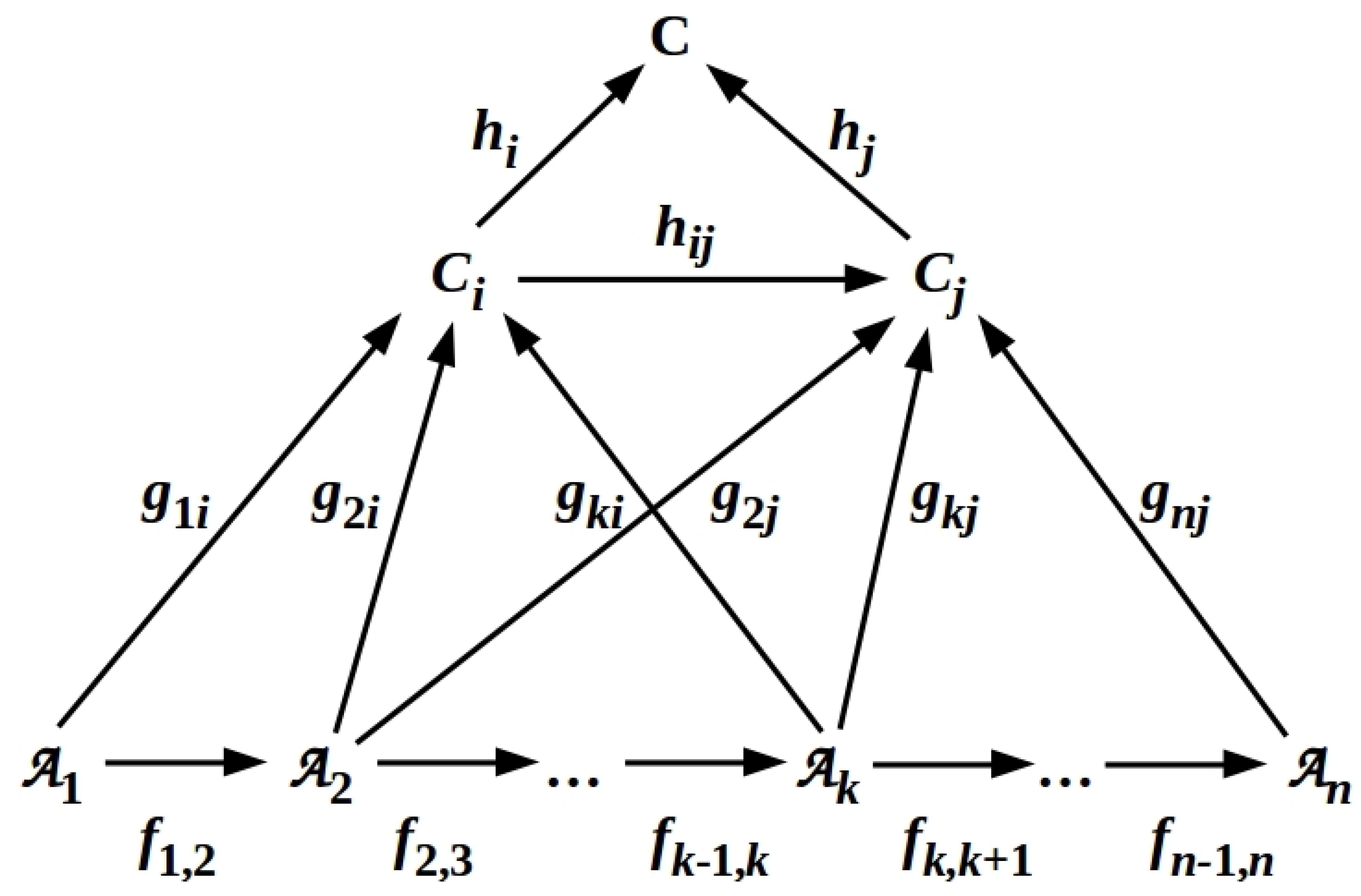
These can be summarized by requiring that all diagrams of the form shown in Figure 3 commute. As the colimit in this case is a cocone over the ${\mathcal{A}}_k$, we refer to such diagrams as “cocone diagrams” (CCDs).

Let us now consider a family of $N^R$ one-bit classifiers

$${\mathcal{A}}_i=<\{e:W(e)\},\{0,1\},{\vDash }_i>$$

(8)

where $W(e)$ if and only if e is an event in W and ${\vDash }_i$ is the ith of $N^R$ distinct, but not necessarily mutually-exclusive, classification criteria. An infomorphism $f_{ij}$ encodes a correlation between the criteria ${\vDash }_i$ and ${\vDash }_j$; if e meets the criterion ${\vDash }_i$, i.e., $e{\vDash }_{i}1$, then $f_{ij}e{\vDash }_{j}1$; otherwise, $f_{ij}e{\vDash }_{j}0$. Infomorphisms are by definition invertible, i.e., $f_{ij}{f}_{ji}=$ Identity; hence, this correlation is bidirectional. Assuming now that a cocone $\mathbf{C}$ above the ${\mathcal{A}}_i$ exists, this $\mathbf{C}$ encodes the information that some event $e\ast$ in W simultaneously satisfies all $N^R$ of the criteria ${\vDash }_i$. It is thus natural to view this $\mathbf{C}$ as identifying events of some type $[e\ast ]$ that satisfy these criteria. Identifying $[e\ast ]$ as “events in which R is present in state $|R\rangle$” this is precisely what the set of mutually-commuting (by Equation (7)) operators $\left\{M_j^R\right\}$ have been defined as doing. We therefore identify the operators $M_j^R$ with classifiers ${\mathcal{A}}_i^R$, and consider the cocone ${\mathbf{C}}^R$ as the definition, for O, of the reference R. As discussed in Section 2.1, we can regard the $M_j^R$ as deployed simultaneously if we coarse-grain time. This identification of the $M_j^R$ as the base of a CCD gives an explicit meaning both to the label R and to the idea that the $M_j^R$ together identify R. As identifying R requires that R be in the fixed state $|R\rangle$, we can also consider the CCD to give an explicit meaning to the idea of identifying R in state $|R\rangle$. This identification process is, as noted above, a computation implemented by $H_O$.

3.3. Measuring the Pointer State $|P\rangle$ of an Identified System S

By identifying R, the observer O by assumption identifies the system S, including its pointer component P. We now turn to the question of measuring the pointer state $|P\rangle$, the state “of interest” of S. We again employ the approach of formally specifying a computational process to be implemented by $H_O$.

Considering the set of measurement operators $\left\{M_k^P\right\}$, it is clear that it can be partitioned into a subsets, each of which contains only operators that mutually commute; in the limit, each of these subsets is a singlet. Moreover, Equation (7) guarantees that any of the $M_k^P$ must commute with all of the $M_j^R$. Hence, we can consider, without loss of generality, measurements made by deploying the $M_j^R$ to identify S, and one of the $M_k^P$ to determine its (perhaps partial) pointer state. As above, the generalization from a single $M_k^P$ to a kth subset ${\left\{M^P\right\}}_k$ of mutually-commuting operators only requires coarse-graining time.

As the selected $M_k^P$ satisfies $[M_k^P,M_j^R]=0,\forall j$, the methods of the previous section can be used to construct a CCD over the $M_j^R$ together with $M_k^P$. We can view the colimit ${\mathbf{C}}_k^R$ in this CCD as encoding the information that P is in state $|P_k\rangle$. In total, we can construct $N^P$ such CCDs. Call the kth such CCD “CCD${}_k$”. We can now ask: What is the relation between the CCD${}_k$, given that the $M_k^P$ generically do not (all) commute? To address this question, we introduce a discrete, coarse-grained time parameter $\tau \ge (N^R+1)\mathsf{\Delta }t$ during which the $M_j^R$ and one or more mutually-commuting $M_k^P$ are executed. We then define an operation ${\mathcal{G}}_{ij}:$ CCD${}_i\to$ CCD${}_j$ that transitions between CCD${}_i$ and CCD${}_j$ in one unit of $\tau$. Physically, this operation ${\mathcal{G}}_{ij}$ can be viewed as a (formal specification of a) discrete sample of the action of the propagator $\mathcal{P}(t)$ appearing in Equation (4).

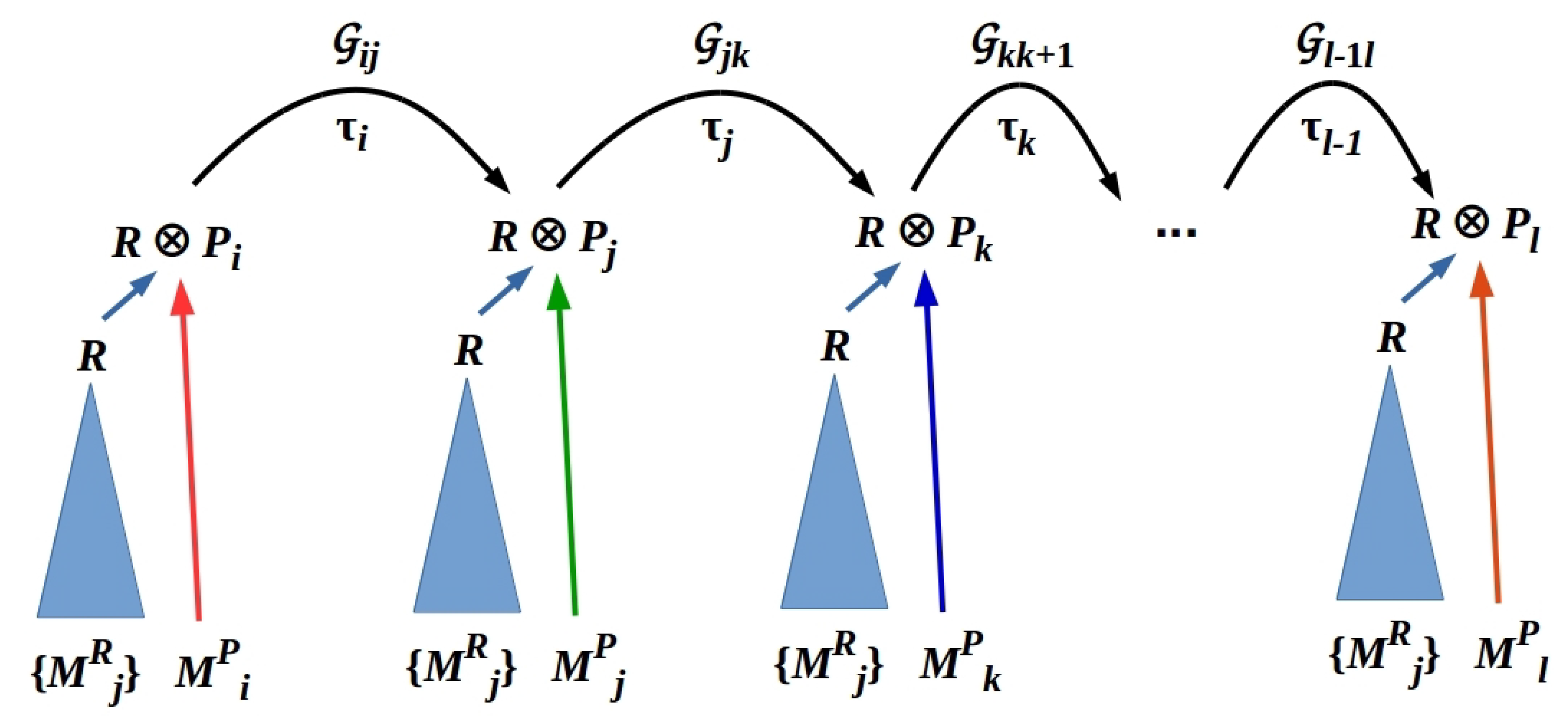
As O can choose to make pointer-state measurements in any order, the operation ${\mathcal{G}}_{ij}$ exists for any i and j. In particular, ${\mathcal{G}}_{ji}$ exists whenever ${\mathcal{G}}_{ij}$ exists. Sequential transitions between CCDs can be represented as compositions, e.g., ${\mathcal{G}}_{ij}\circ {\mathcal{G}}_{jk}$ represents the sequential transition CCD${}_i\to$ CCD${}_j\to$ CCD${}_k$, i.e., a sequence of measurements deploying ${\sum }_j{M}_j^R+M_i^P$, then ${\sum }_j{M}_j^R+M_j^P$, then ${\sum }_j{M}_j^R+M_k^P$, where again we allow $M_i^P$ to also stand for ${\left\{M^P\right\}}_i$ for simplicity. We explicitly assume that ∘ is independent of $\tau$. If $[M_i^P,M_j^P]\ne 0$, then ${\mathcal{G}}_{ij}\circ {\mathcal{G}}_{ji}\ne {\mathcal{G}}_{ji}\circ {\mathcal{G}}_{ij}$. Hence, the elements $\left\{{\mathcal{G}}_{ij}\right\}$ with associative composition ∘ define a groupoid [47,48], not a group. Elements of this groupoid, which we denote $\mathcal{G}$, are labeled by the parameter $\tau$, which distinguishes groupoid actions at distinct times. A sequence of such actions is illustrated in Figure 4.

Clearly a groupoid—indeed, in particular, a permutation group—can also be defined within each CCD${}_k$. The elements of these groupoids ${\mathcal{G}}^k$ are operators ${\mathcal{G}}_{lm}^k$ that exchange the lth and mth elements of the subset $\left\{M_j^R\right\}\cup {\left\{M^P\right\}}_k$ of mutually-commuting measurement operators. These ${\mathcal{G}}^k$ are exchange symmetry groupoids over the elements of their respective subsets $\left\{M_j^R\right\}\cup {\left\{M^P\right\}}_k$. Actions by elements of $\mathcal{G}$ break this exchange symmetry, resulting in decoherence as outlined below.

3.4. Sequential Measurements Induce Decoherence

Let us denote the unmeasured components of P at time ${\tau }_i$ as ${\overline{P}}_i$, so $P=P_i\otimes {\overline{P}}_i$ at ${\tau }_i$. Again $P_i$ can also indicate those components of P measured by an ith subset of mutually-commuting observables. With this notation, at ${\tau }_i$, W comprises a measured system$R\otimes P_i$ and an unmeasured system${\overline{P}}_i\otimes E$, i.e., we have a decomposition $W=(R\otimes P_i)\otimes ({\overline{P}}_i\otimes E)$. The state $|R\otimes P_i\rangle$ is measurable—indeed, it is the pointer state of interest—so $|W\rangle$ must be separable as $|W\rangle =|R\otimes P_i\rangle |{\overline{P}}_i\otimes E\rangle$.

Sequential measurements at ${\tau }_i$ and ${\tau }_j$ swap entanglement of components of P between R and E, i.e., the groupoid elements ${\mathcal{G}}_{ij}$ implement entanglement swaps:

$${\mathcal{G}}_{ij}:|R\otimes P_i\rangle |{\overline{P}}_i\otimes E\rangle \to |R\otimes P_j\rangle |{\overline{P}}_j\otimes E\rangle$$

(9)

Such entanglement swaps implement decoherence [27]. Hence, we can view the groupoid elements ${\mathcal{G}}_{ij}$ as decoherence operators. These operators are implemented by $H_O$, i.e., the observer O decoheres each measured state $|R\otimes P_i\rangle$ by selecting it for measurement and coupling it to its own specific decohering environment ${\overline{P}}_i\otimes E$. The functional asymmetry between the operator subsets $M_i^R$, $M_j^P$, and $M_k^E$ is evident in this representation, as is the asymmetry between the “selected” pointer operators $M_i^P$ and the “unselected” operators $M_j^{\overline{P}}$. The “general” environment E serves as a resource for decoherence that is accessed by O at each measurement.

3.5. Entanglement Swapping Induces Contextuality

The Kochen–Specker theorem [23] shows that quantum theory generically admits contextuality, i.e., the outcome probability distribution obtained for some (subset of) observable(s) can depend on what other observables are simultaneously measured, even when all simultaneously-measured observables mutually commute. Dzhafarov and colleagues have proposed an extension of classical probability theory, termed “contextuality by default” (CbD) in which any measurement system is prescribed in terms of “bunches” of random variables coupled through degrees of connectedness leading to a context label that distinguishes between “true contextuality” on the one hand, and “non-contextual description” on the other [28,29]. The latter typifies the habitual imperfection of empirical systems subject to direct influences, for example, classical signaling between collections of degrees of freedom. “True” contexts distinguish sets of measurements with non-direct influences that can be unpredictable, or indeed empirically unfathomable. Further, it has been shown both that this extension is sufficient to capture Kochen–Specker contextuality [30] and that such contextuality can be observed in human decision making [49] (cf. [50] for an analysis of experiments that only appear to demonstrate contextuality). Effectively, all measured probabilities are expressed as conditioned on some context label c, i.e., $Prob(x)$ becomes $Prob(x|c)$ for any event x measured in c. The context labels in CbD can be viewed simply as a bookkeeping device; there is no formal requirement that the contexts are fully characterized by the available observations.

The unmeasured systems ${\overline{P}}_i\otimes E$ provide natural context labels for comparing outcome probability distributions over the measured systems $R\otimes P_i$. As the outcomes specifying $|R\rangle$ must remain fixed to permit system identification, the outcome probability distributions of interest are of those of the $|P_i\rangle$. If each of the $P_i$ is a one-dimensional component of P, then no observables are measured in multiple contexts and no contextuality is observable. If, however, the $P_i$ are multidimensional components of P, each measured using a subset of mutually-commuting observables ${\left\{M^P\right\}}_i$, contextuality can be expected by default whenever ${\left\{M^P\right\}}_i\cap {\left\{M^P\right\}}_j\ne \varnothing$ for some subsets i and j. The mechanism inducing contextuality is the entanglement swap implemented by the ${\mathcal{G}}_{ij}$ in Equation (9). The special case of noncontextuality only occurs if (in the sense of approximation) $|{\overline{P}}_i\otimes E\rangle \approx |{\overline{P}}_j\otimes E\rangle$, i.e., only if:

$${\mathcal{G}}_{ij}|R\otimes P_i\rangle \approx |R\otimes P_j\rangle$$

(10)

This can occur if and only if $[M_i^P,M_j^P]\approx 0$ for all $M_i^P\in {\left\{M^P\right\}}_i$ and $M_j^P\in {\left\{M^P\right\}}_j$ [30]. It can occur, in other words, only if ${\mathcal{G}}_{ij}$ does not (significantly) break the exchange symmetry within each subset of mutually-commuting operators.

3.6. CCD Commutativity Enforces Bayesian Coherence

As mentioned above, it is now commonplace to consider observers to be Bayesian agents. A Bayesian agent is a system that implements Bayes’ theorem for conditional probabilities, $Prob(a|b)=Prob(b|a)(Prob(a)/Prob(b))$, where a and b are any two events or conditions and $Prob(b)\ne 0$. In the CbD framework, Bayes’ theorem only applies within a context. If probabilities are computed using complex amplitudes for states and the Born rule, contextuality is taken into account via phase interference and Bayes’ theorem can be applied across contexts [38].

While Bayes’ theorem follows from the usual Kolmogorov axioms, following de Finetti [51], it is generally motivated by the rationality of avoiding “Dutch book” probability assignments that violate the Kolmogorov axioms. Assigning probabilities, including conditional probabilities, only in ways that satisfy the Kolmogorov axioms achieves “Bayesian coherence.” Here, we show that if the CCD formalism is extended to include probability labels on observational outcomes, the requirement of commutativity enforces Bayesian coherence and hence compliance with the Kolmogorov axioms.

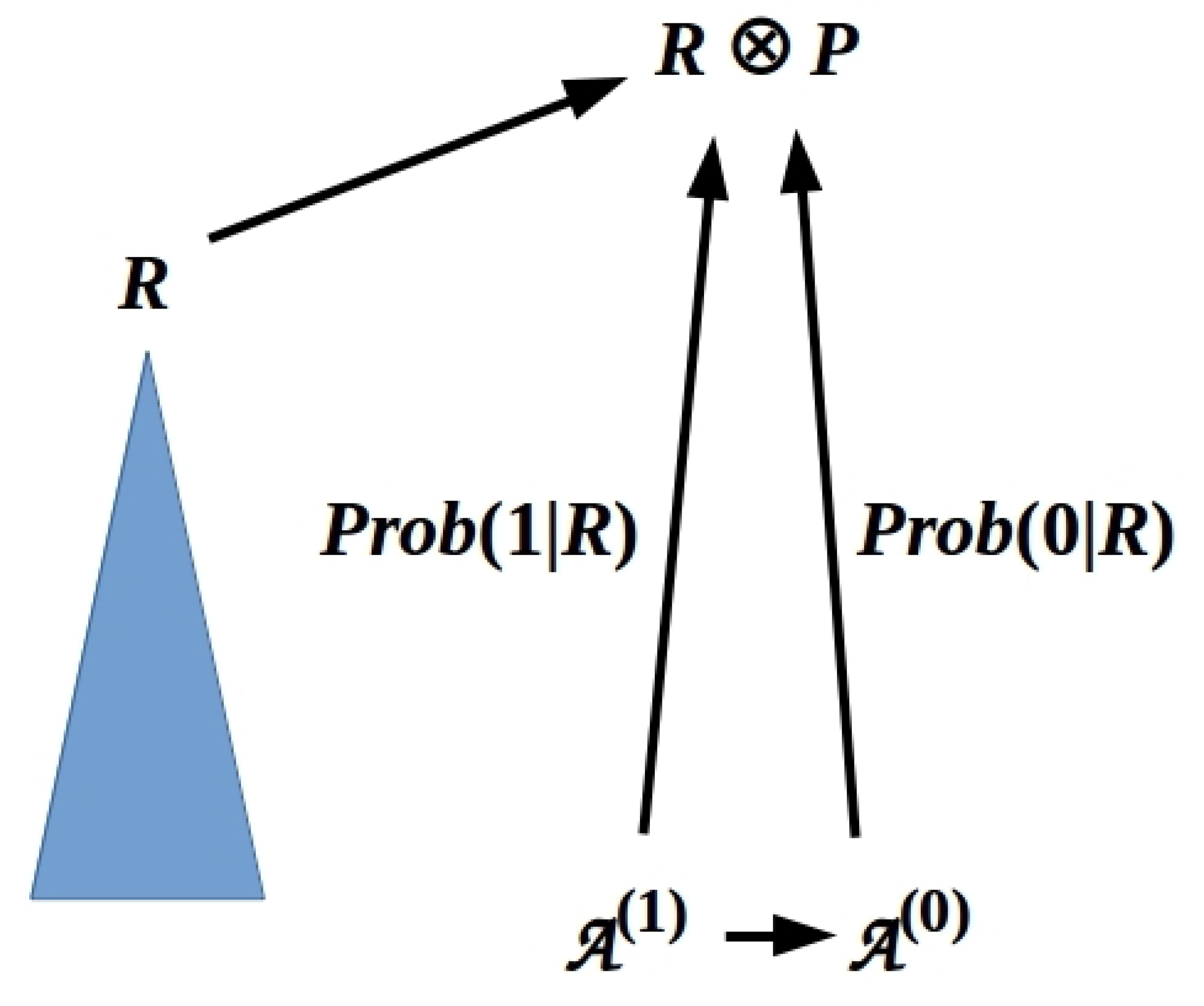
To motivate this, let us represent a single binary measurement somewhat redundantly as implemented by two classifiers, ${\mathcal{A}}^{(1)}$ and ${\mathcal{A}}^{(0)}$, that test for outcomes “1” and “0”, respectively. The probabilities of these outcomes are $Prob$(1$|R$) and $Prob$(0$|R$), respectively; we can treat these probabilities as labels as shown in Figure 5. Here, the horizontal arrow is an infomorphism encoding the classical correlation between ${\mathcal{A}}^{(1)}$ and ${\mathcal{A}}^{(0)}$. Commutativity requires that all paths through the diagram yield the same result; it is natural to extend this requirement to the probability labels by requiring:

• that only the shortest paths between objects in a diagram (such as a CCD) are labeled, and that the probability of a such a path is the product of the probabilities of its component arrows; and
• that the probabilities of all paths sum to unity.

Additivity is thus ensured by commutativity, and conjunction subsumed by conditionals when defined as in Definition 3 below.

Assigning a probability $1/n$ to each horizontal arrow (including right-to-left inverse arrows, even if implicit) between pointer-component classifiers in a diagram with n such classifiers, we have in the case of Figure 5 that $Prob$(1$|R$) $=1-Prob$(0$|R$). Collectively then, the diagram exhibits Bayesian coherence; in particular, the posterior of a prior at one stage can be regarded as the prior for the next [45]. This procedure clearly generalizes to any CCD with n binary pointer-state classifiers (i.e., binary-valued measurement operators) and hence $n^2$ distinct sets of binary-valued observational outcomes. As the state $|R\rangle$ must remain fixed, probabilities are not assigned within the R-identifying cocones of such CCDs.

The idea of “assigning” probabilities to arrows in CCDs over classifiers can be made precise by interpreting classifiers themselves as probabilistic. Following [52] (cf. [53]), we define:

Definition 3.

A sequent $M{\vDash }_{\mathcal{A}}N$ holding of a classifier $\mathcal{A}$ is a pair of subsets $M,N$ of $Typ(\mathcal{A})$ such that $\forall x\in Tok(\mathcal{A})$, $x{\vDash }_{\mathcal{A}}M\to x{\vDash }_{\mathcal{A}}N$.

The sequent relation can be weakened by requiring only that if $x{\vDash }_{\mathcal{A}}M$, there is some probability $Prob(N|M)$ that $x{\vDash }_{\mathcal{A}}N$. This is essentially how a conditional probability interprets the logical implication “⇒” [54] (see [26] for details). If sequents conditioned on R are defined within the colimit classifier $\mathbf{R}\otimes P^k$ of a CCD${}^k$ over a set of pointer-state operators ${\left\{M^P\right\}}_k$ and then relaxed to probabilities, these probabilities can be migrated downward as labels on the infomorphisms from the elements of ${\left\{M^P\right\}}_k$ to $\mathbf{R}\otimes P^k$. As these probabilities are defined within CCD${}^k$, they are CbD compliant with context label k.

4. Thermodynamic Asymmetries and Their Effects

4.1. Information Processing Demands Are Asymmetrical between R, P and E

The formal treatment above admits, via the explicitly thermodynamic representation of $H_{OW}$ in Equation (2), a straightforward physical interpretation in terms of information and resource flows. The environment E is represented in the above as a passive resource for decoherence. The thermodynamic role of E, however, is that of free energy source and waste heat sink. The conversion of free energy to waste heat (“metabolism”) funds the thermodynamically-irreversible state changes of O that are interpretable as “recording” observational outcomes—the “informative” information about W that O is using $H_{OW}$ to discover—on some “memory” implemented by $H_O$. By including the interaction with E as an explicit component of the “measurement” interaction between O and W, Equation (2) avoids the usual “open system” assumption that allows the effects of free-energy extraction and waste-heat dissipation on the measurement process to be neglected. It thus makes the asymmetry between the effects on O of “informative” information flows and “mere” resource flows explicit.

In a simple system with a state trajectory describable as a Markov process, the memory on which observational outcomes are recorded is not persistent for more than one time step $\mathsf{\Delta }t$. However, for “interesting” observers capable of performing multiple observations of the same identified system, memories must persist for multiple time steps. The identification criteria for R, in particular, must persist for multiple time steps in any observer capable of re-identifying R across multiple cycles of measurement. Persistence raises the question of implementation. In a classical system, a memory is persistent only if it has as time-invariant classical record. In a quantum system, however, the classical record of a memory can be erased or modified (i.e., erased and replaced), but it may leave an implicit record of induced phase coherence relations [55]. Such implicit records enable non-Markovian behavior, e.g., Leggett–Garg violations. In the present context, we consider memory of previously-obtained outcomes to be a function of $H_O$, with one effect of memory being the choice of what measurements to make next, e.g., the choice of the functions $n_i^k(t)$ in Equation (5).

Maintaining memories against thermal noise (classical systems) or decoherence (quantum systems) requires the expenditure of free energy. The effective thermodynamic efficiencies $N^R{\beta }^R$ and $N^P{\beta }^P$ of processing measurements of R and P, respectively, must, therefore, incorporate the free-energy demands of maintaining the functional integrity of the virtual-machine architecture described in the last section, however it is implemented by $H_O$. Hence, we can generically expect ${\beta }^R,{\beta }^P\gg 1$, with magnitudes scaling roughly both with $N^R$ and $N^P$, respectively, and with the number of elements of $\mathcal{G}$, i.e., with the complexity of commutativity constraints between the $M_k^P$. Because the time-varying outcomes generated by the $M_k^P$ can be expected to have a larger influence on what is measured next than the time-invariant outcomes generated by the $M_j^R$, we can also generically expect ${\beta }^P>{\beta }^R$. What is “of interest” about an external system S naturally requires more free energy to process, remember, and act upon than what is not [46].

The acquisition of free energy from E must, on the other hand, be relatively efficient if the free energy obtained is to fund information processing (i.e., internal “work”) as well as the “metabolic” processes that convert it to waste heat, i.e., actions back on E or external “work”. Hence, we must generically have $N^E{\beta }^E<N^R{\beta }^R,N^P{\beta }^P$. If we make the reasonable assumption that information processing is somehow compartmentalized in O, e.g., to provide isolation from noise and/or decoherence, a large uniform heat bath will be less efficient as a power source than a smaller, higher-temperature bath local to the processing compartment. We can, therefore, expect that typical O will allocate a component of $H_{OE}$ to high-efficiency free-energy acquisition, i.e., that typically $N^E{\beta }^E=N^{E(h)}{\beta }^{E(h)}+N^{E(l)}{\beta }^{E(l)}$, with $N^{E(h)}{\beta }^{E(h)}\ll N^{E(l)}{\beta }^{E(l)}$, where superscripts h and l indicate high and low efficiency, respectively. Both organisms and apparatus, including all practical computers, employ this compartmentalization strategy ubiquitously.

4.2. Thermodynamic Interactions with E Generically Disturb $|P\rangle$

It is standard to assume that the environment E is “large” even though a large environment is not strictly needed for decoherence [2,10]. One motivation for a large environment is to assure that any classical disturbances to E during the course of observation are well away from the system S of interest and hence negligible.

The assumption of negligible disturbance breaks down, however, when both the thermodynamics of measurement and the mechanism of observer-relative decoherence are taken into account. As shown above, the free energy required per bit to process outcomes obtained by the $M_j^R$ and $M_k^P$ is large compared to $k_B{T}^O$ and hence for typical, near-isothermal measurement interactions, large compared to $k_B{T}^E$, at least in the near vicinity of O. The action in Equation (4) of O on W, and hence on E, is therefore large compared to ℏ. Disturbances to E at the scale of ℏ are insignificant classically, but can be significant to entanglement swaps involving E as in Equation (9). As the swap in Equation (9) is executed every time a new subset of mutually-commuting $M_k^P$ is deployed, these disturbances are not incidental to, but rather are direct consequences of the measurement process. Hence, the action in Equation (4) cannot be considered negligible, but rather must be assumed generically to disturb $|P\rangle$. As shown in [17], the scale of this disturbance increases as the measurement resolution and hence the input bandwidth $N^P$ increases.

5. Discussion

We argue here that the physical interactions that implement observations appear to lose information for a simple and somewhat pedestrian reason: $H_{OW}$ appears not to conserve information because only a (typically small) fraction of the information transferred is considered “informative” by the observer. The rest is, of necessity, employed as free energy to fund the processing and memory storage of the “informative” fraction. In typical discussions of measurement, even the information required to identify R is ignored; only the pointer state is regarded as “of interest” and hence informative, while the rest of the transferred information is relegated to noise or decoherence (e.g., [56], where this is made fully explicit).

When the measurement interaction $H_{OW}$ is considered fully explicitly, two distinct symmetries are broken. Not only are input bits to be processed as information distinguished from input bits to be processed as free-energy supply, but input bits indicating the time-varying pointer state $|P\rangle$ of S must also be distinguished from input bits identifying the reference component of S, the state $|R\rangle$ of which must remain time-invariant. These distinctions in how input bits are processed are reflected by thermodynamic asymmetries, i.e., by the requirement that $N^E{\beta }^E<N^R{\beta }^R,N^P{\beta }^P$ and the generic expectation that ${\beta }^P>{\beta }^R$.

The fundamental asymmetry between R and P is reflected in the architecture of the minimal virtual machine that must be implemented by any observer capable of identifying a system and making a sequence of pointer-state measurements. Simultaneous (in coarse-grained time) measurements of mutually-commuting subsets of observables, including in every instance the $M_j^R$, are processed by a CCD. Switching between mutually-commuting subsets i and j of observables is implemented by a groupoid operator ${\mathcal{G}}_{ij}$. These operators execute entanglement swaps or, equivalently, context swaps. In either picture, they induce decoherence and generically disturb $|P\rangle$.

We do not explicitly consider the operations required to prepare a system S for measurement. We note, however, that preparing S requires identifying S and hence identifying R, and that “measurement settings” are components of P, as illustrated in Figure 2. Preparation requires, in this case, the same operations as measurement; indeed, the two can be considered duals [57]. The dual of a cocone is a cone; combining the two with a single network of classifiers yields a cone–cocone diagram (CCCD) depicting information flow into, through, and then out of the classifier network [26]; it is natural to interpret the limit (of the cone) in a CCCD as a complete prepared state (including R) and the colimit (of the cocone) as a complete measured state, as in Section 3.2. Mutually non-commuting subsets of preparation procedures induce groupoid operations on the cone analogous to the ${\mathcal{G}}_{ij}$.

We emphasize that these results depend only on standard quantum theory, with no assumptions about the structures or properties of O and W beyond the Hilbert-space representation and the assumptions of separability and finiteness specified in the Introduction. They thus apply to any physical system, and depend quantitatively only on the number of degrees of freedom interpretable as subserving memory functions in some form.

We expect the groupoid concept to arise in a similar formalism to the one presented here when equivalence relations are used to classify various types of entanglement [58]. In addition, it has not escaped our notice that CCCDs bear certain structural similarities to another representation of information flow from preparation to measurement, the “amplituhedron” of [59]. This and a deeper understanding of the physical meaning of $\mathcal{G}$ await further work.

References

- Landsman, N.P. Between classical and quantum. In Handbook of the Philosophy of Science: Philosophy of Physics; Butterfield, J., Earman, J., Eds.; Elsevier: Amsterdam, The Netherlands, 2007; pp. 417–553. [Google Scholar]
- Schlosshauer, M. Decoherence and the Quantum to Classical Transition; Springer: Berlin, Germany, 2007. [Google Scholar]
- Bohr, N. The quantum postulate and the recent development of atomic theory. Nature 1928, 121, 580–590. [Google Scholar] [CrossRef] [Green Version]
- Fröwis, F.; Sekatski, P.; Dür, W.; Gisin, N.; Sangouard, N. Macroscopic quantum states: Measures, fragility, and implementations. Rev. Mod. Phys. 2018, 90, 025004. [Google Scholar] [CrossRef] [Green Version]
- Schrödinger, E. The present situation in quantum mechanics. Naturwissenschaften 1980, 23, 807–812. (In German) (English translation by Trimmer, J. D. Proc. Am. Phil. Soc. 1980, 124, 323–328) [Google Scholar] [CrossRef]
- Wigner, E.P. Remarks on the mind-body question. In The Scientist Speculates; Good, I.J., Ed.; Heinemann: London, UK, 1961; pp. 284–302. [Google Scholar]
- Mermin, D. Hidden variables and the two theorems of John Bell. Rev. Mod. Phys. 1993, 65, 803–815. [Google Scholar] [CrossRef]
- Zurek, W.H. Decoherence, einselection and the existential interpretation (the rough guide). Philos. Trans. R. Soc. A 1998, 356, 1793–1821. [Google Scholar] [CrossRef] [Green Version]
- Zurek, W.H. Decoherence, einselection, and the quantum origins of the classical. Rev. Mod. Phys. 2003, 75, 715–775. [Google Scholar] [CrossRef] [Green Version]
- Schlosshauer, M. Quantum decoherence. Phys. Rep. 2019, 831, 1–57. [Google Scholar] [CrossRef] [Green Version]
- Ollivier, H.; Poulin, D.; Zurek, W.H. Environment as a witness: Selective proliferation of information and emergence of objectivity in a quantum universe. Phys. Rev. A 2005, 72, 042113. [Google Scholar] [CrossRef] [Green Version]
- Chiribella, G.; D’Ariano, G.M. Quantum information becomes classical when distributed to many users. Phys. Rev. Lett. 2006, 97, 250503. [Google Scholar] [CrossRef] [Green Version]
- Zurek, W.H. Quantum Darwinism. Nat. Phys. 2009, 5, 181–188. [Google Scholar] [CrossRef]
- Korbicz, J.K.; Horodecki, P.; Horodecki, R. Objectivity in a noisy photonic environment through quantum state information broadcasting. Phys. Rev. Lett. 2014, 112, 120402. [Google Scholar] [CrossRef] [PubMed] [Green Version]
- Fields, C. Quantum Darwinism requires an extra-theoretical assumption of encoding redundancy. Int. J. Theor. Phys. 2010, 49, 2523–2527. [Google Scholar] [CrossRef] [Green Version]
- Kastner, R.E. ‘Einselection’ of pointer observables: The new H-theorem? Stud. Hist. Phil. Mod. Phys. 2014, 48, 56–58. [Google Scholar] [CrossRef] [Green Version]
- Fields, C. Some consequences of the thermodynamic cost of system identification. Entropy 2018, 20, 797. [Google Scholar] [CrossRef] [Green Version]
- Ghirardi, G.C.; Rimini, A.; Weber, T. Unified dynamics for microscopic and macroscopic systems. Phys. Rev. D 1986, 34, 470–491. [Google Scholar] [CrossRef]
- Penrose, R. On gravity’s role in quantum state reduction. Gen. Relativ. Gravit. 1996, 28, 581–600. [Google Scholar] [CrossRef]
- Weinberg, S. Collapse of the state vector. Phys. Rev. A 2012, 85, 062116. [Google Scholar] [CrossRef] [Green Version]
- Wheeler, J.A. Law without law. In Quantum Theory and Measurement; Wheeler, J.A., Zurek, W.H., Eds.; Princeton University Press: Princeton, NJ, USA, 1983; pp. 182–213. [Google Scholar]
- Emary, C.; Lambert, N.; Nori, F. Leggett-Garg inequalities. Rep. Prog. Phys. 2013, 77, 016001. [Google Scholar] [CrossRef]
- Kochen, S.; Specker, E.P. The problem of hidden variables in quantum mechanics. J. Math. Mech. 1967, 17, 59–87. [Google Scholar] [CrossRef]
- Landauer, R. Irreversibility and heat generation in the computing process. IBM J. Res. Dev. 1961, 5, 183–195. [Google Scholar] [CrossRef]
- Barwise, J.; Seligman, J. Information Flow: The Logic of Distributed Systems; Cambridge Tracts in Theoretical Computer Science 44; Cambridge University Press: Cambridge, UK, 1997. [Google Scholar]
- Fields, C.; Glazebrook, J.F. A mosaic of Chu spaces and Channel Theory I: Category-theoretic concepts and tools. J. Expt. Theor. Artif. intell. 2019, 31, 177–213. [Google Scholar] [CrossRef]
- Fields, C. Decoherence as a sequence of entanglement swaps. Results Phys. 2019, 12, 1888–1892. [Google Scholar] [CrossRef]
- Dzhafarov, E.N.; Kujala, J.V.; Cervantes, V.H. Contextuality-by-default: A brief overview of concepts and terminology. In Lecture Notes in Computer Science 9525; Atmanspacher, H., Filik, T., Pothos, E., Eds.; Springer: Heidelberg, Germany, 2016; pp. 12–23. [Google Scholar]
- Dzhafarov, E.N.; Kujala, J.V. Contextuality-by-Default 2.0: Systems with binary random variables. In Lecture Notes in Computer Science 10106; Barros, J.A., Coecke, B., Pothos, E., Eds.; Springer: Berlin, Germany, 2017; pp. 16–32. [Google Scholar]
- Dzharfarov, E.N.; Kon, M. On universality of classical probability with contextually labeled random variables. J. Math. Psych. 2018, 85, 17–24. [Google Scholar] [CrossRef] [Green Version]
- Bartlett, S.D.; Rudolph, T.; Spekkens, R.W. Reference frames, superselection rules, and quantum information. Rev. Mod. Phys. 2007, 79, 555–609. [Google Scholar] [CrossRef] [Green Version]
- Gell-Mann, M.; Hartle, J.B. Quantum mechanics in the light of quantum cosmology. In Foundations of Quantum Mechanics in the Light of New Technology; Nakajima, S., Murayama, Y., Tonomura, A., Eds.; World Scientific: Singapore, 1997; pp. 347–369. [Google Scholar]
- Fields, C.; Marcianò, A. Sharing nonfungible information requires shared nonfungible information. Quant. Rep. 2019, 1, 252–259. [Google Scholar] [CrossRef] [Green Version]
- Zanardi, P. Virtual quantum subsystems. Phys. Rev. Lett. 2001, 87, 077901. [Google Scholar] [CrossRef] [Green Version]
- Zanardi, P.; Lidar, D.A.; Lloyd, S. Quantum tensor product structures are observable-induced. Phys. Rev. Lett. 2004, 92, 060402. [Google Scholar] [CrossRef] [Green Version]
- Dugić, M.; Jeknić, J. What is “system”: Some decoherence-theory arguments. Int. J. Theor. Phys. 2006, 45, 2215–2225. [Google Scholar] [CrossRef] [Green Version]
- Dugić, M.; Jeknić, J. What is “system”: The information-theoretic arguments. Int. J. Theor. Phys. 2008, 47, 805–813. [Google Scholar] [CrossRef] [Green Version]
- Fuchs, C.A.; Schack, R. Quantum-bayesian coherence. Rev. Mod. Phys. 2013, 85, 1693–1715. [Google Scholar] [CrossRef] [Green Version]
- Leifer, M.S.; Spekkens, R.W. Towards a formulation of quantum theory as a causally neutral theory of Bayesian inference. Phys. Rev. A 2013, 88, 052130. [Google Scholar] [CrossRef] [Green Version]
- Fields, C. If physics is an information science, what is an observer? Information 2012, 3, 92–123. [Google Scholar] [CrossRef] [Green Version]
- Mueller, M.P. Law without law: From observer states to physics via algorithmic information theory. arXiv 2019, arXiv:1712.01826v4. [Google Scholar]
- Realpe-Gómez, J. Modeling observers as physical systems representing the world from within: Quantum theory as a physical and self-referential theory of inference. arXiv 2019, arXiv:1705.04307v4. [Google Scholar]
- Smith, J.E.; Nair, R. The architecture of virtual machines. IEEE Comput. 2005, 38, 32–38. [Google Scholar] [CrossRef] [Green Version]
- Nielsen, M.A.; Chuang, I.L. Quantum Computation and Quantum Information; Cambridge University Press: New York, NY, USA, 2000. [Google Scholar]
- Fields, C.; Glazebrook, J.F. A mosaic of Chu spaces and Channel Theory II: Applications to object identification and mereological complexity. J. Expt. Theor. Artif. Intell. 2019, 31, 237–265. [Google Scholar] [CrossRef]
- Roederer, J. Information and Its Role in Nature; Springer: Berlin, Germany, 2005. [Google Scholar]
- Weinstein, A. Groupoids: Unifying internal and external symmetry. Notices AMS 1996, 43, 744–752. [Google Scholar]
- Brown, R. Topology and Groupoids; Ronald Brown: Deganwy, UK, 2006. [Google Scholar]
- Cervantes, V.H.; Dzhafarov, E.N. Snow Queen is evil and beautiful: Experimental evidence for probabilistic contextuality in human choices. Decision 2018, 5, 193–204. [Google Scholar] [CrossRef]
- Dzhafarov, E.N.; Zhang, R.; Kujala, J. Is there contextuality in behavioural and social systems? Philos. Trans. R. Soc. A 2016, 374, 20150099. [Google Scholar] [CrossRef]
- De Finetti, B. Theory of Probability, Vol. I; Wiley: New York, NY, USA, 1974. [Google Scholar]
- Allwein, G.; Moskowitz, I.S.; Chang, L.-W. A New Framework for Shannon Information Theory; Technical Report A801024; Naval Research Laboratory: Washington, DC, USA, 2004.
- Seligman, J. Channels: From logic to probability. In Formal Theories of Information; Sommaruga, G., Ed.; Lecture Notes in Computer Science, 5363; Springer: Berlin, Geramny, 2009; pp. 193–233. [Google Scholar]
- Adams, E.W. A Primer of Probabilistic Logic; University of Chicago Press: Chicago, IL, USA, 1998. [Google Scholar]
- Nielsen, M.A.; Chuang, I.L. Quantum Information and Quantum Computation; Cambridge University Press: Cambridge, UK, 2000. [Google Scholar]
- Tegmark, M. How unitary cosmology generalizes thermodynamics and solves the inflationary entropy problem. Phys. Rev. D 2012, 85, 123517. [Google Scholar] [CrossRef] [Green Version]
- Pegg, D.; Barnett, S.; Jeffers, J. Quantum theory of preparation and measurement. J. Mod. Opt. 2002, 49, 913–924. [Google Scholar] [CrossRef] [Green Version]
- Walter, M.; Gross, D.; Eisert, J. Multi-partite entanglement. In Lectures on Quantum Information; Bruss, D., Leuchs, D., Eds.; Wiley-VCH: Weinheimm, Germany, 2006. [Google Scholar]
- Arkani-Hamed, N.; Trnka, J. The amplituhedron. J. High Energy Phys. 2014, 10, 030. [Google Scholar] [CrossRef] [Green Version]
Figure 1.
Observer O and world W exchange bits via an ancillary array of non-interacting qubits. Bit values are preserved if a quantum reference frame (here, a z axis) is shared a priori.
Figure 2.
To be identifiable by observation, a system S must have a reference component R with a time-invariant state . To be of interest for measurements, S must also have a pointer component P with a time-varying state .
Figure 3.
A cocone diagram (CCD) is a commuting diagram depicting maps (infomorphisms) between classifiers and , maps from the to one or more channels over a subset of the , and maps from channels to the colimit (cf. Equation (6.7) of [26]).
Figure 4.
A sequence of CCDs identifying R (blue triangles) and measuring pointer components . Transitions between CCDs are implemented by groupoid elements, e.g., and labeled by discrete times, e.g., . The operators can equally well be generalized to subsets of mutually-commuting pointer-state observables.
Figure 5.
Bayesian coherence is obtained if probabilities along all paths in a diagram sum to unity. Probabilities are not assigned within the R-identifying cocone (blue triangle).
© 2020 by the authors. Licensee MDPI, Basel, Switzerland. This article is an open access article distributed under the terms and conditions of the Creative Commons Attribution (CC BY) license (http://creativecommons.org/licenses/by/4.0/).
Share and Cite
MDPI and ACS Style
Fields, C.; Glazebrook, J.F. Representing Measurement as a Thermodynamic Symmetry Breaking. Symmetry 2020, 12, 810. https://0-doi-org.brum.beds.ac.uk/10.3390/sym12050810
AMA Style
Fields C, Glazebrook JF. Representing Measurement as a Thermodynamic Symmetry Breaking. Symmetry. 2020; 12(5):810. https://0-doi-org.brum.beds.ac.uk/10.3390/sym12050810
Chicago/Turabian StyleFields, Chris, and James F. Glazebrook. 2020. "Representing Measurement as a Thermodynamic Symmetry Breaking" Symmetry 12, no. 5: 810. https://0-doi-org.brum.beds.ac.uk/10.3390/sym12050810
Note that from the first issue of 2016, this journal uses article numbers instead of page numbers. See further details here.