Forecasting of Coalbed Methane Daily Production Based on T-LSTM Neural Networks


1
College of Resources and Environment, University of Chinese Academy of Sciences, Beijing 100049, China
2
School of Earth Sciences and Engineering, Hohai University, Nanjing 211000, China
3
Key Laboratory of Computational Geodynamics, College of Earth and Planetary Sciences, University of Chinese Academy of Sciences, Beijing 100049, China
*
Authors to whom correspondence should be addressed.
Symmetry 2020, 12(5), 861; https://0-doi-org.brum.beds.ac.uk/10.3390/sym12050861
Submission received: 30 April 2020
/
Revised: 14 May 2020
/
Accepted: 19 May 2020
/
Published: 23 May 2020
(This article belongs to the Special Issue Mathematical Modeling and Computational Methods in Science and Engineering II)
Abstract
:Accurately forecasting the daily production of coalbed methane (CBM) is important forformulating associated drainage parameters and evaluating the economic benefit of CBM mining. Daily production of CBM depends on many factors, making it difficult to predict using conventional mathematical models. Because traditional methods do not reflect the long-term time series characteristics of CBM production, this study first used a long short-term memory neural network (LSTM) and transfer learning (TL) method for time series forecasting of CBM daily production. Based on the LSTM model, we introduced the idea of transfer learning and proposed a Transfer-LSTM (T-LSTM) CBM production forecasting model. This approach first uses a large amount of data similar to the target to pretrain the weights of the LSTM network, then uses transfer learning to fine-tune LSTM network parameters a second time, so as to obtain the final T-LSTM model. Experiments were carried out using daily CBM production data for the Panhe Demonstration Zone at southern Qinshui basin in China. Based on the results, the idea of transfer learning can solve the problem of insufficient samples during LSTM training. Prediction results for wells that entered the stable period earlier were more accurate, whereas results for types with unstable production in the early stage require further exploration. Because CBM wells daily production data have symmetrical similarities, which can provide a reference for the prediction of other wells, so our proposed T-LSTM network can achieve good results for the production forecast and can provide guidance for forecasting production of CBM wells.
1. Introduction
As a high-quality energy source that can replace natural gas, coalbed methane (CBM) is an important energy reserve in China [1]. The rational use and drainage of CBM is significant for improving energy structure, protecting the environment, and promoting economic development [2]. Forecasting CBM daily production can not only help predict the economic benefits of CBM development [3], but also provide a basis for development of reasonable parameters for CBM drainage, which plays an important role in the orderly mining of CBM [4].
At present, methods for predicting the daily production of CBM mainly include type curves, decline curves, numerical simulations, material balance [5], and machine learning (e.g., neural networks, support vector machines (SVMs)).
Li et al. [6] used the Weibull curve to make a segmented prediction of CBM production, obtaining a better fit in linear regression. Xu et al. [7] introduced the relationship between type curve–dimensionless production and time, proposing the type curve method of CBM production by analyzing the influence of permeability and Langmuir pressure on the type curve. Jang et al. [8] predicted production performance of CBM by combining falling curve analysis with material balance and flow analysis to establish a comprehensive production data model of CBM. In addition, several scholars have studied CBM production using multivariate regression methods. For example, Xu et al. [4] established a prediction model for outflows of CBM by combining multivariate regression with contour analysis of the coalbed floor. Chen et al. [9] used the main factors affecting the gas content of coal seams extracted through correlation analysis into the multivariate stepwise regression to produce a predicted value consistent with the measured value. Li et al. [10] combined stepwise regression with a variety of factors to make quantitative predictions about CBM resources.
Numerical simulations of unconventional gas reservoirs are summarized in the works of Cipolla et al. [11], which often employ relatively complex mathematical models. With developments in relevant technologies, geological parameters and human influence factors now require increasing consideration to improve model accuracy. For example, Zhao et al. [12] used a gray lattice Boltzmann method to perform numerical simulations, so as to address the problem of interlayer interference caused by changes in permeability and differences in pressure between coal seams during the mining process. Zhou [13] also used numerical simulations to predict the production of a horizontal CBM well in Australia. The works of Cipolla et al. [11] also reflect this trend, often employing complex mathematical models to numerically simulate the output of unconventional gas reservoirs. Yun et al. [1] used C++-based Korean software CBMRS 1.0 to develop their own software dedicated to providing numerical CBM reservoir simulation. Accurate geological parameters and sufficient production data are essential to the use of numerical simulations for production forecasting [14]; without these, the use of numerical simulations would be inappropriate.
The material balance equation is also an important tool for estimating the reserves and performance of both conventional and unconventional gas reservoirs. King [15] introduced two material balance methods for unconventional gas reservoirs that considered the effects of adsorbed gas; these were used to estimate natural gas reserves and reservoir predictions. By contrast, the material balance equations proposed by Shi et al. [16] considered the effects of the difference between initial reservoir pressure and critical desorption pressure, pore and water compressibility, and dissolved and free gas factors. Sun et al. [17] proposed an improved flow material balance (FMB) equation method by taking into account the pressure–saturation relationship, which provides a reliable tool for extracting low-permeability CBM reservoir information. As evidenced by these advancements, material balance equation methods for CBM production forecasting can take into account numerous factors; however, CBM production is a complex and dynamic process that is not limited to the aforementioned factors, and the difficulty of obtaining these hinders the performance of these methods.
Machine learning methods avoid discussion of complex geological conditions as well as human factors, allowing for more convenient applications in production forecasting. For example, many scholars [18,19,20,21] have used BP neural networks to predict CBM production and have found that neural networks are more accurate than the traditional method. Xia et al. [22] proposed a mixed method based on a rough set (RS) and least squares support vector machine (LS-SVM) to predict CBM productivity. Existing methods for predicting CBM production have been used widely, and a majority have established a complex mathematical model for production forecasting. However, CBM production is a complex dynamic process, influenced by several factors. This, coupled with the unavailability of several factors, makes the process difficult to describe using a mathematical model [2]. Although machine learning methods such as BP neural networks and SVMs have a wide range of applications in production forecasting, predicting CBM production is a typical time series problem based on historical production data of gas wells. BP neural networks and other methods do not fully consider the time dependence of time series data, analyze only a single sample’s data [23], and are very susceptible to errors.
Although the process of CBM mining is extremely complicated, the daily production of CBM itself is the result of a combination of various factors, which to some extent reflects the internal mechanism of the system [24]. Accordingly, it is possible to abandon complicated research and find out the inherent change rule based on historical data by studying daily CBM production data, then predict future output. Aiming at the time series variation rule of CBM production data, this study proposes a prediction method of CBM production based on long short-term memory (LSTM) models. The main contribution of this paper is to propose a Transfer-LSTM (T-LSTM) model for predicting CBM production. It innovatively applies transfer learning (TL) to the LSTM network pretraining process and has achieved good results.
2. Related Work
LSTM is suitable for analyzing time series, being a deep learning recurrent neural network structure that can learn long-term sequence data [25]. With the development of deep learning, the LSTM model has achieved satisfactory results in many aspects. In time series prediction, for example, many scholars [25,26,27,28] have applied the LSTM model to predict the fine particulate matter (PM2.5) concentration of air pollution and obtained more accurate predictions than by existing methods. Chen [29], Tian [30], and Li et al. [31] studied traffic flow using an LSTM model. Ma et al. [32] used LSTM and Beijing microwave traffic detection data to predict traffic speed and found that a LSTM network predicted accuracy and stability better than traditional neural network and other parametric or nonparametric algorithms did. Fischer [33] and Kim et al. [34] used the LSTM model to make predictions about financial markets and found that the results were better than the results of random forest, deep neural network (DNN), and other methods. Peng [35] and Fang et al. [36] used the LSTM model to predict electricity prices and electricity sales. Sagheer et al. [37] proposed a deep long short-term memory (DLSTM) oil production prediction method based on genetic algorithm optimization and compared it with statistical and software calculation methods, finding that the proposed DLSTM model was more accurate under different comparison standards. Wang [3] analyzed the time series of mine gas leakage based on the deep learning method but did not predict CBM production. Although LSTM models have been widely used in time series analysis, they are still relatively new in CBM production forecasting. In this study, the LSTM model was applied to predict CBM production, leading to discussion of the feasibility of using deep learning to predict CBM production.
3. Data and Methods
3.1. Data Description
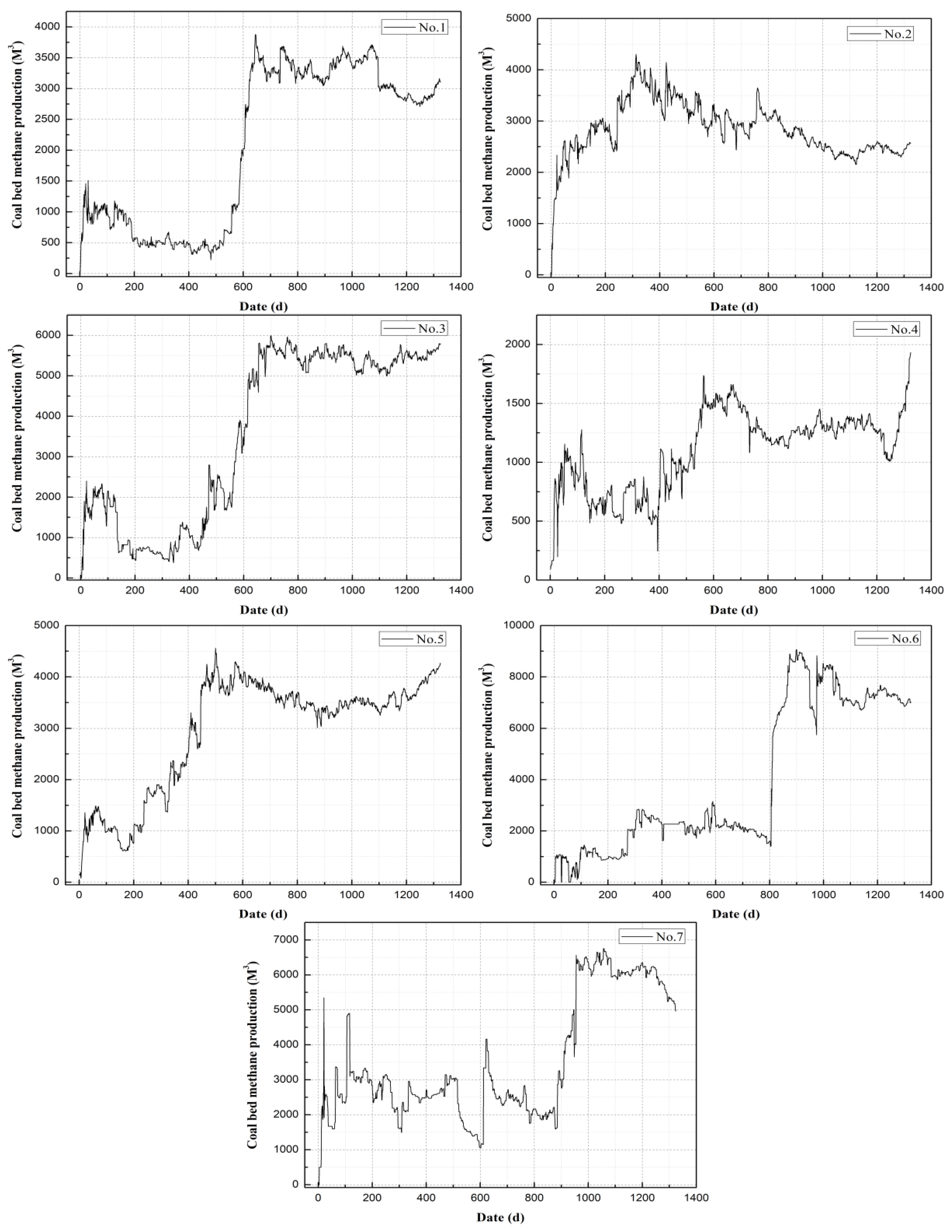
The experimental datasets used in this study were the CBM production data of the Panhe Demonstration Zone of Qinnan CBM in Jincheng, Shanxi, China. The first phase of the demonstration area was put into operation in 2005. Through years of drainage, the CBM production of these CBM wells has entered a stable stage. The dataset consists of two parts: the first includes multiple indicators such as CBM production, bottom hole temperature, casing pressure, water production, coal seam structure, coal seam thickness, and the like for 149 gas wells from 2005 to 2010. The second part contains the CBM production of another 7 gas wells from 2011 to 2014. Because these data are the earliest successful commercialized CBM drainage data in China, analysis of the production data of the early wells can guide the exploitation of new wells. In this study, we mainly tested the CBM production of the seven wells in the second part. Because CBM production data for seven wells are insufficient for deep learning network training, we used the first part of the data to pretrain the network and used transfer learning (see Section 3.2 of this paper) to predict the second part of the CBM production. The time series of CBM production in the seven wells is shown in Figure 1, where X indicates the number of days of CBM mining (1, 2, 3…, n) and y represents daily CBM production (m3). It can be seen from the curves that the CBM output types of the seven wells are different and vary greatly with different phases.
The data were divided into training sets and test sets as required. To ensure availability of sufficient data to train the network, the dataset was divided into training sets and test sets in the ratio of 80% and 20%, respectively. To avoid the impact of excessive numerical range on the accuracy of the network, CBM datasets were first standardized to values ranging between 0 and 1. Normalization of the data is conducive to initialization and adjustment of learning rate and can greatly improve neural networks’ speed in finding an optimal solution [38]. The min–max normalization method was adopted in this paper.
3.2. LSTM Neural Network
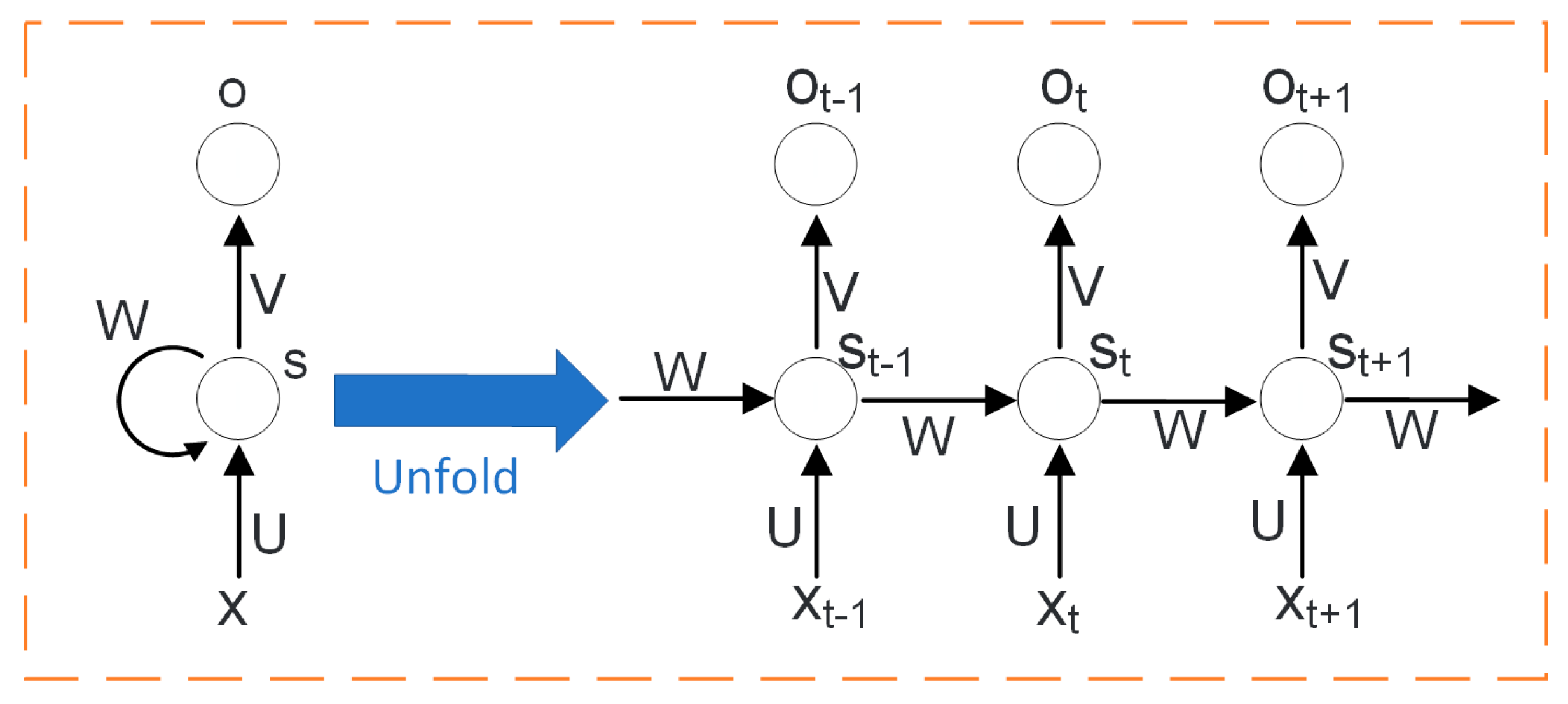
LSTM is a special kind of recurrent neural network (RNN) that can effectively solve the gradient disappearance or explosion problem of RNN through long-term dependence of time series analysis [39,40,41,42,43,44,45]. Unlike traditional neural networks, RNN has hidden nodes that are connected, with the current output of a time series related to the output before it, so that the time sequence characteristics of data can be taken into account. The structure of a typical RNN network is shown in Figure 2. The left side represents a network element, and the right side is the unfolded form of multiple network elements, where t represents a time series, X input values, and St memory at time t. W, U, and V represent the weights of the input, the moment, and the output, respectively, and O represents the output values. RNN can capture timing features but can solve only short-sequence problems; it does not work for long-sequence data such as CBM daily production.
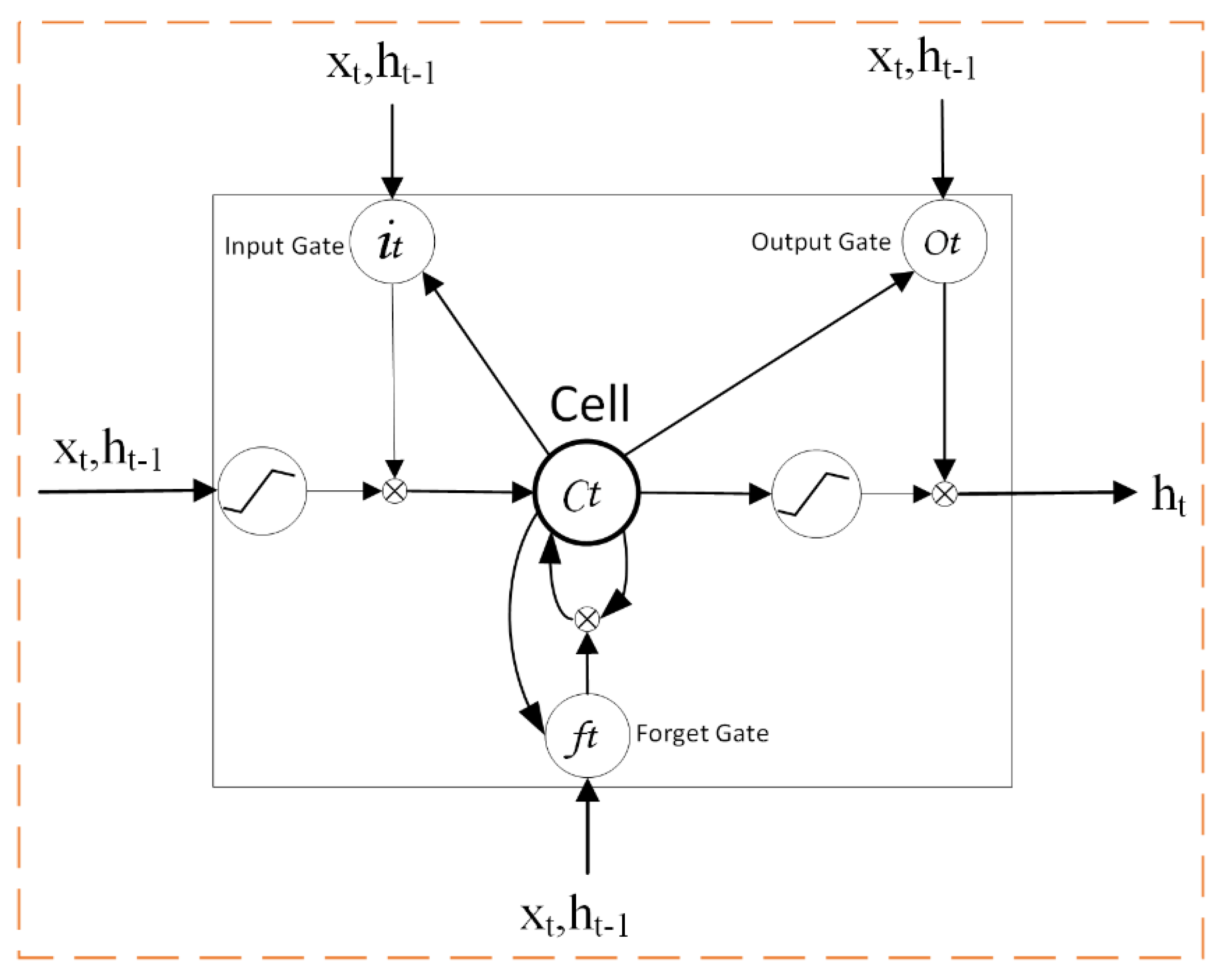
LSTM can overcome the shortcomings of RNN and features long-term memory. A typical LSTM network cell structure is shown in Figure 3, where Cell represents a memory cell; Xt and ht represent the input and output at time t, respectively; and ht–1 represents the output at the previous time. The LSTM network structure solves the RNN gradient problem through three “gates”: a “forget gate”, an “input gate”, and an “output gate”. The “forget gate” decides which information to discard and which to retain, the “input gate” controls the information input to the cell, and the “output gate” controls the output information. The hidden layer structure of the LSTM network can be calculated by the following equations:
where t is a time series; i, f, c, and o are input gate, forget gate, output gate, and memory cell, respectively; W and b are corresponding weights and offsets, respectively; and ó represents a sigmoid function.
According to the characteristics of CBM time series data, the overall framework of predicting CBM daily production using the LSTM model is shown in Figure 4. The framework of CBM production time series prediction was divided into three parts: input layer, hidden layer, and output layer. The input layer was responsible for data standardization and dividing the datasets. The data output from the input layer was used as an input to the hidden layer. The hidden layer was used to build the LSTM network structure and predict the time series data. The hidden layer was antistandardized by the output layer after completing the prediction, and the prediction results were used as the output.
We used mean absolute error (MAE), mean absolute percentage error (MAPE), and root mean square error (RMSE) as the three principal indicators to evaluate the accuracy of our experiments,
where Pi is predicted CBM production, Ai is actual CBM production, and n is number of test samples.
3.3. T-LSTM Model
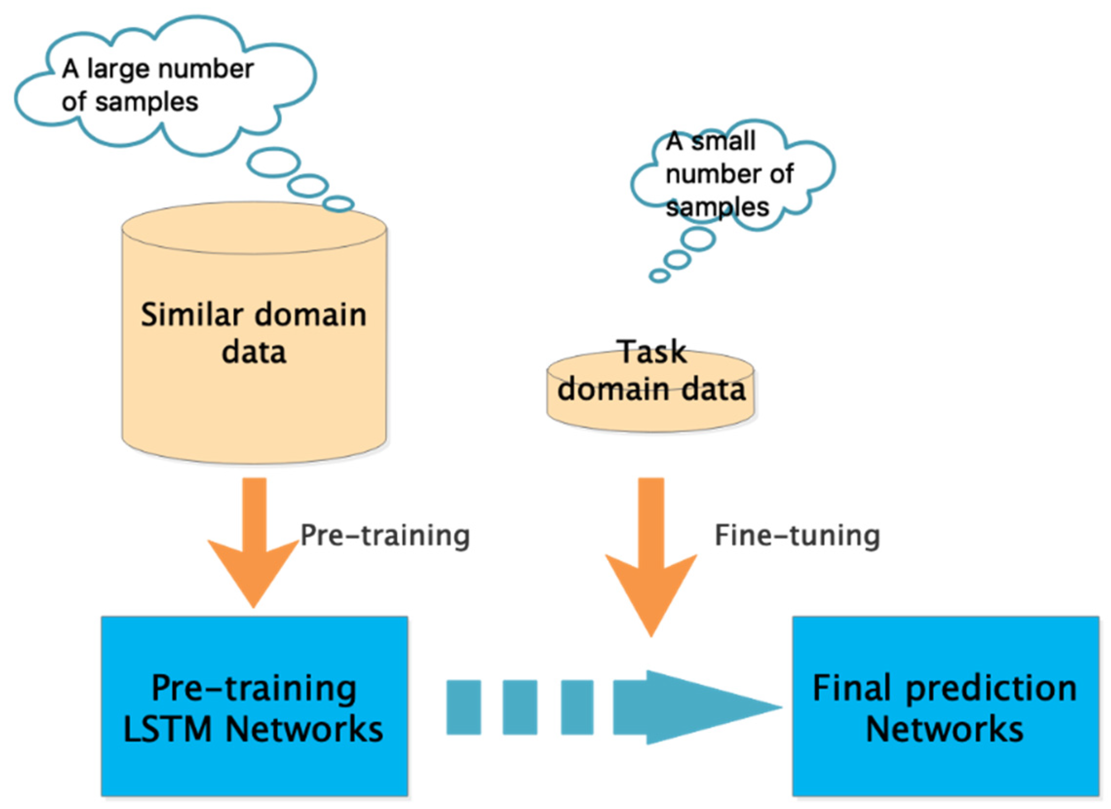
Transfer learning applies knowledge learned in a similar domain to a target domain to make up for an insufficient number of samples in the actual training process. The similar domain refers to the existing knowledge, whereas the target domain is the new knowledge to be learned. In our study, the similar domain is the data for the 149 wells in the first part, and the target domain is the data for the 7 wells in the second part. Obviously, a dataset of 7 gas wells is relatively sparse for deep learning training. Compared with our target data, a dataset of 149 gas wells is relatively large, so we use the transfer learning method to apply the knowledge learned on 149 gas wells to the target domain. Although the data in the similar domain are not from the same period as our target 7 gas wells, they all have similar periodic characteristics and are very similar to our task domain [6]. Accordingly, we can first use gas production data for 149 wells to pretrain our network, fix the learned weights, then transfer our findings to the target domain, using gas production data in the target domain to fine-tune the network parameters. In this way, we have formed a new T-LSTM model. Through transfer learning, we can largely solve the problem of insufficient samples for deep learning. The specific process is shown in Figure 5:
4. T-LSTM Network Training and Parameter Optimization
The training set was used as an input into the T-LSTM network model for training, and the model parameters were optimized through experiments. Here, well 4 is taken as an example to explain the setting of the parameters. First, the influence of the number of LSTM hidden layers on network training and prediction results was explored. The input layer and output layer of the network were set to 1. Based on past experience, the initial learning rate was set to 0.001, the number of nodes in each layer was 128, and the training iteration times epoch was set to 300.
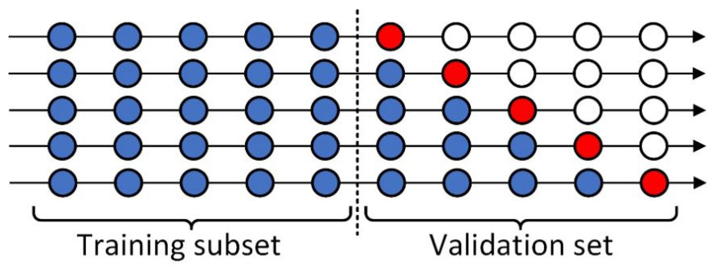
Cross-validation is needed for optimal parameter selection. For machine learning and deep learning, there are many traditional cross-validation methods, such as the leave-one-out cross-validation method and the k-fold cross-validation method [46,47]. However, these methods cannot be used in time series prediction, because time series data are time-dependent. To solve this problem, rolling-origin recalibration evaluation was adopted in this paper [48]. The training set was divided into two parts, with the first 50% the training subset and the second 50% the validation set. In the forward rolling validation, the data from the validation set were moved to the training subset in chronological order. Our cross-validation process is shown in Figure 6, with blue circles representing training data, red circles validation data, and hollow circles unused data. We performed a split of the validation set five times, each time using 10% of the data for verification and then moving it to the training subset in chronological order for the next training process.
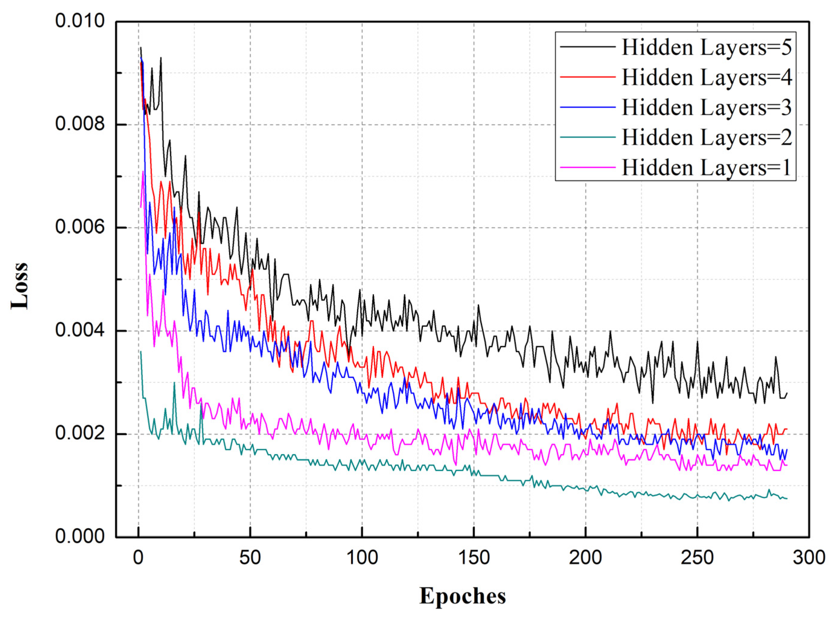
The optimal number of hidden layers was selected by experiments from 1 to 5. To improve the generalization ability of the model and prevent overfitting, the dropout function was included in the LSTM model and 20% of the nodes were discarded. The loss function used was MSE. Corresponding to the different numbers of hidden layers (1, 2, 3, 4, 5), the LSTM network was trained, and the number of hidden layers was selected by comparing the loss variation of the model, as shown in Figure 7. As can be seen from Figure 7, with two hidden layers, the loss obtained was at its minimum (less than 0.001). Accordingly, two hidden layers were selected to train the LSTM model. The more hidden layers used, the longer the network training time required. Accordingly, using more hidden layers in a network does not necessarily produce better network training. As can be seen from the results, use of too many layers not only reduces training accuracy but also greatly increases training time.
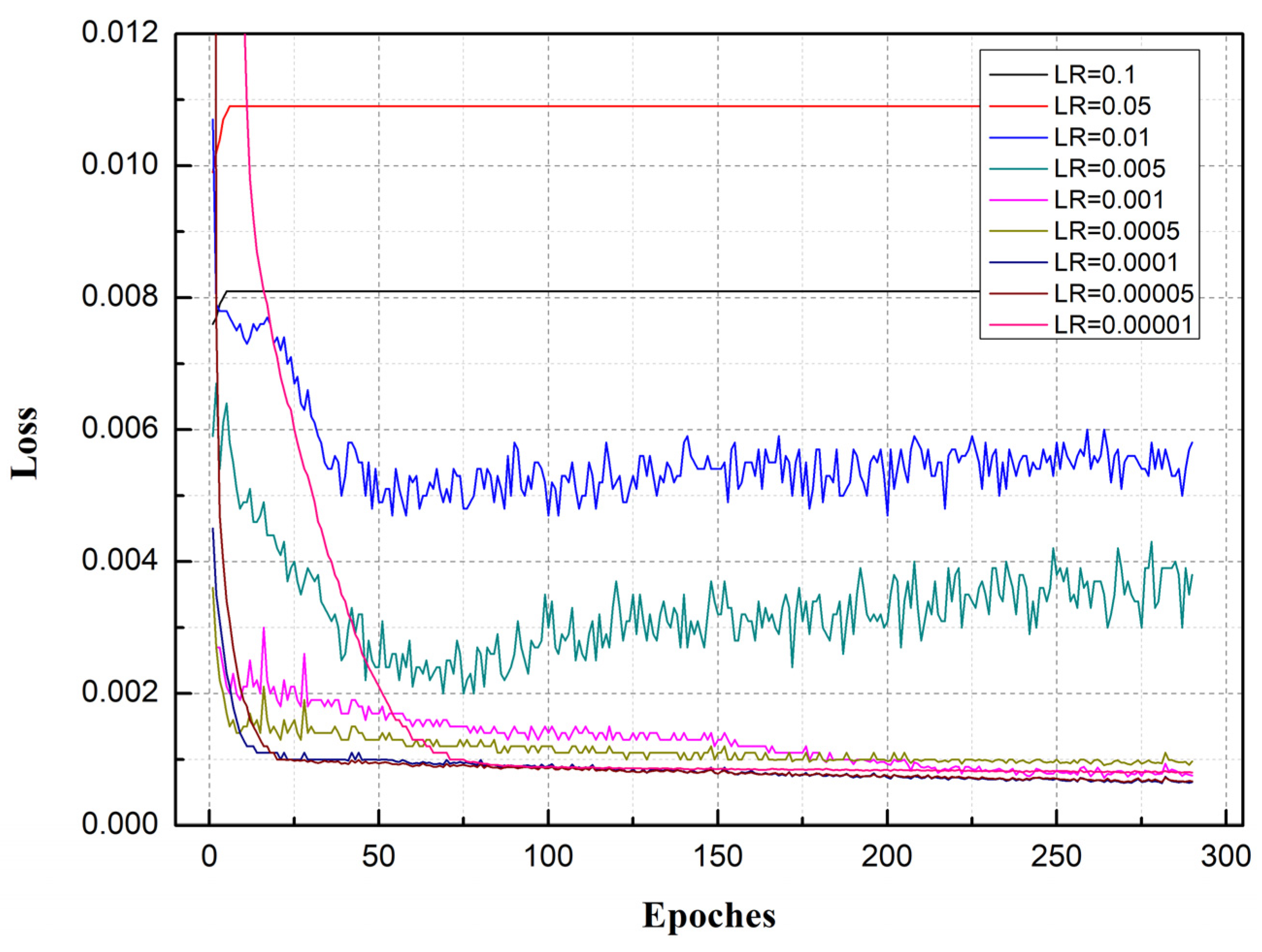
The learning rate was found to directly affect the training result of the model. If the learning rate was too high, the model was not trained accurately. Conversely, too small a learning rate increased network convergence time. Through experimentation, the hidden layer’s number of LSTM networks was fixed at 2, and different values of the learning rate were taken (LR = 0.00001, 0.00005, 0.0001, 0.0005, 0.001, 0.005, 0.01, 0.05, and 0.1) to explore the influence of learning rate value on the model. The variations in model loss, corresponding to different learning rates, are shown in Figure 8. As can be seen, when the learning rate was large (LR = 0.1, 0.05), the loss of the model did not gradually decrease with the epoch but rather increased to a certain value and stopped changing as the epoch increased. The model fit was poor. As the learning rate gradually decreased (LR = 0.01, 0.005), the loss error gradually decreased as the epoch increased. However, as the epoch continued to increase, loss error increased instead of decreasing and was mostly in a state of shock. When the learning rate decreased to 0.001, loss value decreased with increases in epoch and gradually stabilized. When the learning rate decreased to 0.0001, loss value reached its minimum value (less than 0.001) and model accuracy its highest value (with RMSE, MAE, and MAPE at their minimum values). As the learning rate continued to decrease, the loss value no longer decreased significantly but the precision of the model started to decrease (RMSE, MAE, and MAPE became larger). These findings show that when LR = 0.0001, the model can achieve a better fit and achieve the highest accuracy. Accordingly, a learning rate of 0.0001 was adopted to train the LSTM network.
Based on the foregoing analysis, we used a network with two hidden layers and set the learning rate to 0.0001.
5. Results and Discussion
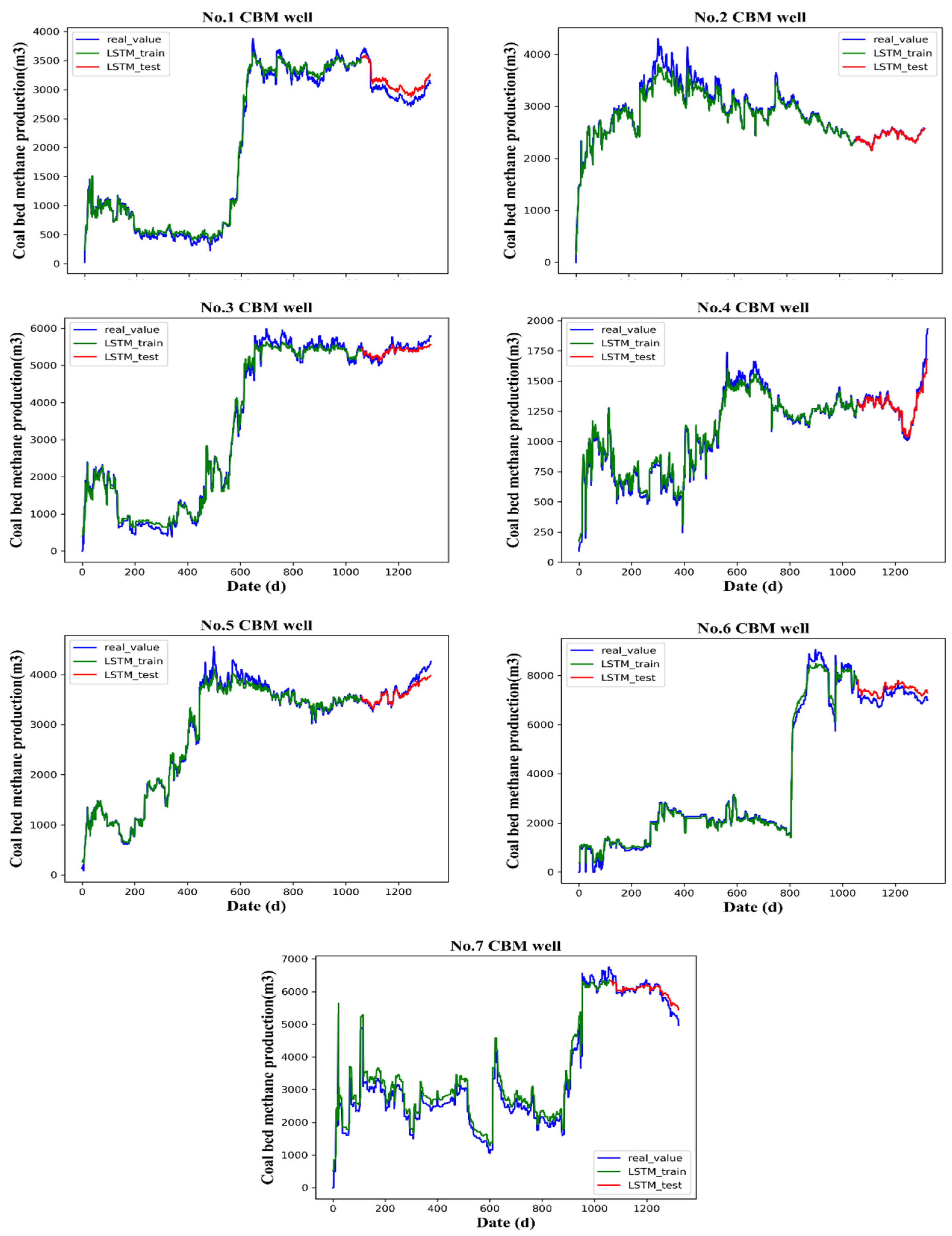
We trained the T-LSTM model through cross-validation and finally determined the optimal structure and parameters of the network. Then, the LSTM model was used to predict the CBM production of seven wells. The final prediction of CBM production is shown in Figure 9 (No. 1–No. 7), with blue representing measured data, green the LSTM network output result of the training set, and red the prediction of the T-LSTM network for the test set. It can be seen that time series analysis of daily CBM production by T-LSTM can achieve accurate results. The predicted CBM production by the T-LSTM network was close to the actual production. The predicted production of wells 2 and 4 was the most consistent with actual production. From the results, the predicted values are evenly distributed on both sides of the true values, indicating that the predicted results are unbiased. Although the results for wells 1, 6 and 7 were significantly lower than those of other sample areas, the predicted values deviated farther from the true values, the overall estimated values were higher than the true values, and the predicted results were biased.
The RMSE, MAE, and MAPE values of the seven CBM wells were statistically analyzed, as shown in Table 1. As can be seen, the errors of wells 2, 3, 4, and 5 were small, with RMSE values of 25.79, 90.86, 47.33, and 89.02, respectively, whereas the errors of wells 1, 6, and 7 were large, with RMSE values of 155.04, 174.53, and 184.06, respectively.
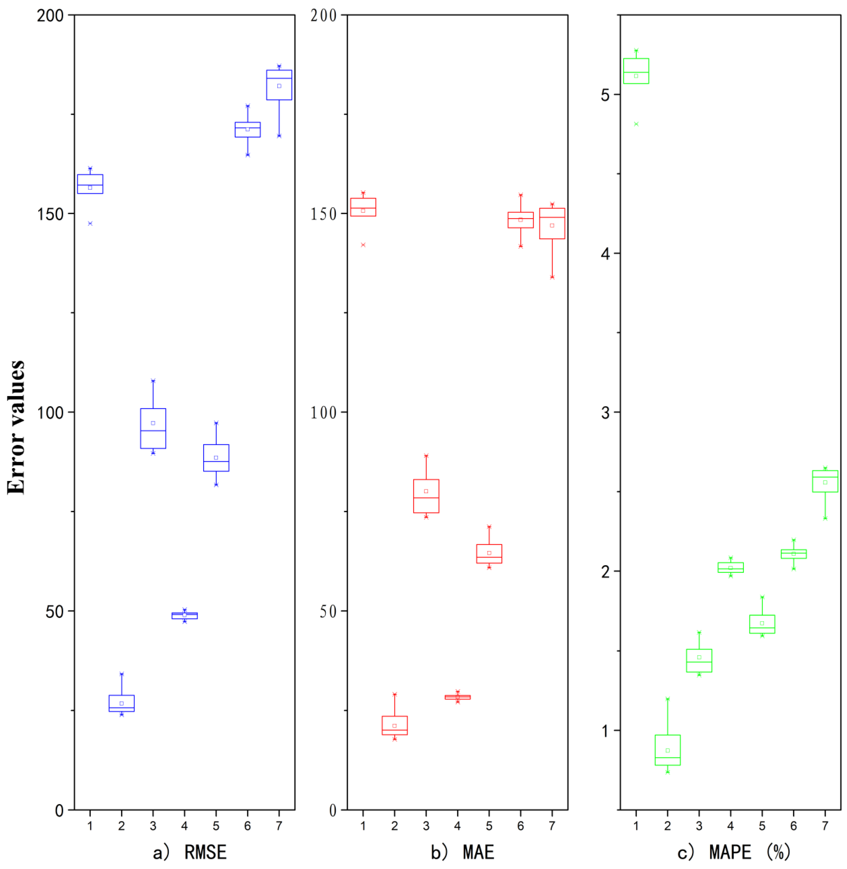
For the LSTM network, different results were obtained by each network training. To avoid the contingency of network training and develop a robust LSTM network, 30 independent repeat experiments were conducted on the CBM production data for each gas well. After setting the network parameters, training for each well was repeated 30 times, with RMSE, MAE, and MAPE values obtained for each repeat. Then boxplots were used to statistically analyze the RMSE of the 30 experiments, with RMSE, MAE, and MAPE distributions used to verify the stability of the T-LSTM network. Thirty independent repetitions sufficed to obtain a good distribution of these three indicators. The boxplots for the seven wells are shown in Figure 10. It can be seen that the RMSE, MAE, and MAPE results obtained from the 30 network trainings were concentrated, with a small interval between the upper and lower quartiles indicating a small distribution range and good stability of the LSTM network. From the boxplots, we can clearly see that the prediction result for well 2 was the most accurate, featuring the smallest RMSE, MAE, and MAPE values. The prediction results for wells 1, 6, and 7 were relatively poor, featuring large values of RMSE, MAE, and MAPE. Based on analysis of the change curves of production with time, the gas production of well 2 entered the stage of stable and continuous CBM production earlier, so the prediction result was relatively accurate. However, for types such as well 6, having low output or unstable output at the early stage, neural networks have not yet learned the characteristics of the time series of the curves well, making it difficult to grasp the time node of the output change and thus to forecast results for these types with a high degree of accuracy.
In addition, we compared the T-LSTM model with other CBM production prediction cases in the literature, as shown in Table 2. As can be seen, the average relative error of the T-LSTM model we proposed is 2.20%. The prediction error of the T-LSTM model was smaller than most cases in the references, indicating that the T-LSTM model can predict CBM production better than many traditional methods. Moreover, the T-LSTM model is more convenient to operate than traditional methods. It does not require consideration of many complex geological factors and complex mathematical models, only input of historical production data, and thus can be more efficient than many traditional methods.
6. Conclusions
In this study, a time series forecasting method of CBM daily production based on a T-LSTM network has been proposed, and parameter selection and model training, with CBM production forecasting of the T-LSTM model introduced. Through experimentation, the following findings were made:
(1) The use of the T-LSTM model for time series forecasting of CBM production can provide accurate results. Compared with traditional methods, the LSTM model does not need to consider the complex mining process of CBM but instead directly looks for the rule from the time series data to predict future output. Combining the idea of transfer learning with that of LSTM can solve the problem of insufficient training samples for deep learning. It can be seen from the experiment that the curve of CBM production predicted by the T-LSTM model was very close to the actual production curve and that error was small, suggesting a significant role for this model in practical applications.
(2) When training the LSTM model, the number of hidden layers and the setting of learning rate are very important. With too few hidden layers, the model could not be fully trained. Too many layers increased the network training time and reduced efficiency. Too large or too small learning rates will affect network convergence speed and can even lead to overfitting and underfitting. Accordingly, multiple experiments are needed to find the most suitable value.
(3) When predicting CBM production in seven gas wells, it can be seen that the prediction accuracy of gas wells with different periodic trends varies greatly. For gas wells that entered the stable production period earlier, the T-LSTM model’s predicted results were more accurate. However, for gas well types that showed unstable production for a long time in the early stage, or that had extremely low production and suddenly increased at a certain stage, the prediction results were relatively poor. CBM production of these types of wells has not yet produced a regular rule, and as a result, the neural network has not been fully trained, showing that LSTM might not be suitable for predicting production of all types of CBM wells—a finding that requires further exploration.
Author Contributions
X.X. modelled the T-LSTM network, analyzed data and drew the main conclusions. X.R. summarized the framework of the article, reviewed the related work and sorted through most of the references. Y.F. improved the parameter settings. T.Y. provided the cross-validation strategy and assisted with the revision. Finally, Y.J. preprocessed the data and provided the main dataset for prediction. All authors have read and agreed to the published version of the manuscript.
Funding
This research was financially supported by the National Key Research and Development Program of China (Grant No. 2016YFC0600510), the Fundamental Research Funds for the Central Universities (Grant No. 2019B02514), the National Science and Technology Major Project of China (Grant No. 2017ZX05064005; 2016ZX05066006), the Strategic Priority Research Program of the Chinese Academy of Sciences (Grant No. XDA05030100), and the National Natural Science Foundation of China (Grant No. 41771478).
Conflicts of Interest
The authors declare no conflict of interest.
References
- Yun, M.G.; Rim, M.W.; Han, C.N. A model for pseudo-steady and non-equilibrium sorption in coalbed methane reservoir simulation and its application. J. Nat. Gas Sci. Eng. 2018, 54, 342–348. [Google Scholar] [CrossRef]
- Xu, H. Research on Particle Swarm Optimization Algorithm Improvement and Its Application in the CBM Production Forecast; China University of Mining and Technology: Jiangsu, China, 2013. [Google Scholar]
- Wang, S.Q. Gas Time Series Prediction and Anomaly Detection Based on Deep Learning; China University of Mining and Technology: Jiangsu, China, 2018. [Google Scholar]
- Ping, X.; Xiaochun, L.; Zhiming, F.; Bing, B. Application of Quantification Theory to predict Coal Methane Content. Disaster Adv. 2012, 5, 1609–1614. [Google Scholar]
- Clarkson, C. Production data analysis of unconventional gas wells: Review of theory and best practices. Int. J. Coal Geol. 2013, 109, 101–146. [Google Scholar] [CrossRef]
- Li, H.; Li, Z.; Zhang, H.; Hu, J.T. Study of Coalbed Methane Production Forecast at Different Stages by Using Weibull Model. J. Oil Gas Technol. 2013, 35, 100–103. [Google Scholar]
- Xu, B.X.; Li, X.F.; Hu, X.H.; Hu, S.M. Type curves for production prediction of coalbed methane wells. J. China Univ. Min. Technol. 2011, 40, 743–747. [Google Scholar]
- Jang, H.; Kim, Y.; Park, J.; Lee, J. Prediction of production performance by comprehensive methodology for hydraulically fractured well in coalbed methane reservoirs. Int. J. Oil Gas Coal Technol. 2019, 20, 143–168. [Google Scholar] [CrossRef]
- Chen, X.J.; Li, P.F.; Li, P.; Hui, P.; Guo, Y.H. Application of Multiple Stepwise Regression Analysis in Prediction of Coal Seam Gas Content (in Chinese). Coal Eng. 2019, 51, 106–111. [Google Scholar]
- Li, D.; Cheng, S.; Wang, Z. The Prediction on Coal Field’s CBM (Coalbed Methane) Resource (in Chinese). Shanxi Sci. Technol. 2015, 1, 54–56. [Google Scholar]
- Cipolla, C.L.; Lolon, E.P.; Erdle, J.C.; Rubin, B. Reservoir Modeling in Shale-Gas Reservoirs. SPE Reserv. Eval. Eng. 2010, 13, 638–653. [Google Scholar] [CrossRef]
- Zhao, Y.-L.; Zhao, L.; Wang, Z.-M.; Yang, H. Numerical simulation of multi-seam coalbed methane production using a gray lattice Boltzmann method. J. Pet. Sci. Eng. 2019, 175, 587–594. [Google Scholar] [CrossRef]
- Zhou, F. History matching and production prediction of a horizontal coalbed methane well. J. Pet. Sci. Eng. 2012, 96, 22–36. [Google Scholar] [CrossRef]
- Lü, Y.; Tang, D.; Xu, H.; Tao, S. Productivity matching and quantitative prediction of coalbed methane wells based on BP neural network. Sci. China Ser. E Technol. Sci. 2011, 54, 1281–1286. [Google Scholar] [CrossRef]
- King, G. Material-Balance Techniques for Coal-Seam and Devonian Shale Gas Reservoirs with Limited Water Influx. SPE Reserv. Eng. 1993, 8, 67–72. [Google Scholar] [CrossRef]
- Shi, J.; Chang, Y.; Wu, S.; Xiong, X.; Liu, C.; Feng, K. Development of material balance equations for coalbed methane reservoirs considering dewatering process, gas solubility, pore compressibility and matrix shrinkage. Int. J. Coal Geol. 2018, 195, 200–216. [Google Scholar] [CrossRef]
- Sun, Z.; Shi, J.; Zhang, T.; Wu, K.; Miao, Y.; Feng, D.; Sun, F.; Han, S.; Wang, S.; Hou, C.; et al. The modified gas-water two phase version flowing material balance equation for low permeability CBM reservoirs. J. Pet. Sci. Eng. 2018, 165, 726–735. [Google Scholar] [CrossRef]
- Liu, Z.; Yang, X.; Zhang, J. Logging Predicting for Coalbed Gas Content in Eastern Block of Ordos Basin. Geol. Sci. Technol. Inf. 2014, 33, 95–99. [Google Scholar]
- Xu, H.; Tang, D.Z.; Liu, D.M.; Tang, S.H.; Yang, F.; Chen, X.Z.; He, W.; Deng, C.M. Study on coalbed methane well productivity by using artificial neural network (in Chinese). China Coal 2012, 38, 9–13. [Google Scholar]
- Lv, Y.M.; Tang, D.Z.; Li, Z.P.; Shao, X.J.; Hu, H. Fitting and predicting models for coalbed methane wells dynamic productivity (in Chinese). J. China Coal Soc. 2011, 36, 1481–1485. [Google Scholar]
- Ma, X.; Zhang, C.; Chen, X.F. A Method Combined Principal Component Analysis and BP Artifical Neural Network for Coalbed Methane (CBM) Wells to Predict Productivity (in Chinese). Sci. Technol. Ind. 2013, 13, 97–100. [Google Scholar]
- Xia, H.; Qin, Y.; Zhang, L.; Cao, Y.; Xu, J. Forecasting of coalbed methane (CBM) productivity based on rough set and least squares support vector machine. In Proceedings of the 2017 25th International Conference on Geoinformatics, Buffalo, NY, USA, 2–4 August 2017; pp. 1–6. [Google Scholar]
- Li, C.S.; Tan, M.X.; Zhang, K.J. Research on Single Well Production Prediction Based on Improved BP Neural Networks (in Chinese). Sci. Technol. Eng. 2011, 11, 7766–7769. [Google Scholar]
- Yang, Y.G.; Qin, Y. Study and application on random dynamic model of the coalbed methane output forecasting (in Chinese). J. China Coal Soc. 2001, 2, 122–125. [Google Scholar]
- Bai, Y.; Zeng, B.; Li, C.; Zhang, J. An ensemble long short-term memory neural network for hourly PM2.5 concentration forecasting. Chemosphere 2019, 222, 286–294. [Google Scholar] [CrossRef] [PubMed]
- Li, X.; Peng, L.; Yao, X.; Cui, S.; Hu, Y.; You, C.; Chi, T. Long short-term memory neural network for air pollutant concentration predictions: Method development and evaluation. Environ. Pollut. 2017, 231, 997–1004. [Google Scholar] [CrossRef] [PubMed]
- Wen, C.; Liu, S.; Yao, X.; Peng, L.; Li, X.; Hu, Y.; Chi, T. A novel spatiotemporal convolutional long short-term neural network for air pollution prediction. Sci. Total. Environ. 2019, 654, 1091–1099. [Google Scholar] [CrossRef]
- Zhao, J.; Deng, F.; Cai, Y.; Chen, J. Long short-term memory - Fully connected (LSTM-FC) neural network for PM2.5 concentration prediction. Chemosphere 2019, 220, 486–492. [Google Scholar] [CrossRef]
- Zhao, Z.; Chen, W.; Wu, X.; Chen, P.C.Y.; Liu, J. LSTM network: A deep learning approach for short-term traffic forecast. IET Intell. Transp. Syst. 2017, 11, 68–75. [Google Scholar] [CrossRef] [Green Version]
- Tian, Y.; Zhang, K.; Li, J.; Lin, X.; Yang, B. LSTM-based traffic flow prediction with missing data. Neurocomputing 2018, 318, 297–305. [Google Scholar] [CrossRef]
- Li, Y.; Cao, H. Prediction for Tourism Flow based on LSTM Neural Network. Procedia Comput. Sci. 2018, 129, 277–283. [Google Scholar] [CrossRef]
- Ma, X.; Tao, Z.; Wang, Y.; Yu, H.; Wang, Y. Long short-term memory neural network for traffic speed prediction using remote microwave sensor data. Transp. Res. Part C Emerg. Technol. 2015, 54, 187–197. [Google Scholar] [CrossRef]
- Fischer, T.; Krauss, C. Deep learning with long short-term memory networks for financial market predictions. Eur. J. Oper. Res. 2018, 270, 654–669. [Google Scholar] [CrossRef] [Green Version]
- Kim, H.Y.; Won, C.H. Forecasting the volatility of stock price index: A hybrid model integrating LSTM with multiple GARCH-type models. Expert Syst. Appl. 2018, 103, 25–37. [Google Scholar] [CrossRef]
- Peng, L.; Liu, S.; Liu, R.; Wang, L. Effective long short-term memory with differential evolution algorithm for electricity price prediction. Energy 2018, 162, 1301–1314. [Google Scholar] [CrossRef]
- Fang, Z.Q.; Wang, X.H.; Xia, T. Electricity Sales Forecasting Based on Long-short Term Memory Networks. Electr. Power Eng. Technol. 2018, 37, 78–83. (In Chinese) [Google Scholar]
- Sagheer, A.; Kotb, M. Time series forecasting of petroleum production using deep LSTM recurrent networks. Neurocomputing 2019, 323, 203–213. [Google Scholar] [CrossRef]
- Chen, Z.; Mauricio, A.; Li, W.; Gryllias, K. A deep learning method for bearing fault diagnosis based on Cyclic Spectral Coherence and Convolutional Neural Networks. Mech. Syst. Signal Process. 2020, 140, 1–16. [Google Scholar] [CrossRef]
- Chemali, E.; Kollmeyer, P.; Preindl, M.; Ahmed, R.; Emadi, A.; Kollmeyer, P. Long Short-Term Memory Networks for Accurate State-of-Charge Estimation of Li-ion Batteries. IEEE Trans. Ind. Electron. 2017, 65, 6730–6739. [Google Scholar] [CrossRef]
- Cortez, B.; Carrera, B.; Kim, Y.-J.; Jung, J.-Y. An architecture for emergency event prediction using LSTM recurrent neural networks. Expert Syst. Appl. 2018, 97, 315–324. [Google Scholar] [CrossRef]
- Kumar, J.; Goomer, R.; Singh, A.K. Long Short Term Memory Recurrent Neural Network (LSTM-RNN) Based Workload Forecasting Model For Cloud Datacenters. Procedia Comput. Sci. 2018, 125, 676–682. [Google Scholar] [CrossRef]
- Li, C.; Wang, Z.; Rao, M.; Belkin, D.; Song, W.; Jiang, H.; Yan, P.; Li, Y.; Lin, P.; Hu, M.; et al. Long short-term memory networks in memristor crossbar arrays. Nat. Mach. Intell. 2019, 1, 49–57. [Google Scholar] [CrossRef]
- Petersen, N.C.; Rodrigues, F.; Pereira, F.C. Multi-output bus travel time prediction with convolutional LSTM neural network. Expert Syst. Appl. 2019, 120, 426–435. [Google Scholar] [CrossRef] [Green Version]
- Gao, W.; Farahani, M.R.; Aslam, A.; Hosamani, S. Distance learning techniques for ontology similarity measuring and ontology mapping. Clust. Comput. 2017, 20, 959–968. [Google Scholar] [CrossRef]
- Xiong, Z.; Wu, Y.; Ye, C.; Zhang, X.; Xu, F. Color image chaos encryption algorithm combining CRC and nine palace map. Multimedia Tools Appl. 2019, 78, 31035–31055. [Google Scholar] [CrossRef]
- Cordero, A.; Jaiswal, J.P.; Torregrosa, J.R. Stability analysis of fourth-order iterative method for finding multiple roots of non-linear equations. Appl. Math. Nonlinear Sci. 2019, 4, 43–56. [Google Scholar] [CrossRef] [Green Version]
- Voit, M.; Meyer-Ortmanns, H. Predicting the separation of time scales in a heteroclinic network. Appl. Math. Nonlinear Sci. 2019, 4, 279–288. [Google Scholar] [CrossRef] [Green Version]
- Bergmeir, C.; Benítez, J.M. On the use of cross-validation for time series predictor evaluation. Inf. Sci. 2012, 191, 192–213. [Google Scholar] [CrossRef]
Figure 1.
Time series of coalbed methane (CBM) daily production for the seven wells.

Figure 2.
Structure of recurrent neural network (RNN).

Figure 3.
Long short-term memory (LSTM) neural network hidden layer cell structure.

Figure 4.
Framework of time series forecasting of CBM production based on LSTM. A recursive arrow indicates that the processing can be repeated.
Figure 4.
Framework of time series forecasting of CBM production based on LSTM. A recursive arrow indicates that the processing can be repeated.

Figure 5.
The process of transfer learning.

Figure 6.
The process of cross-validation.

Figure 7.
Loss curves comparison with different numbers of hidden layers.

Figure 8.
Loss curve comparison with different learning rates.

Figure 9.
Predictions of daily CBM production by T-LSTM model.

Figure 10.
RMSE, MAE, and MAPE error boxplots of 30 T-LSTM network training for seven wells.


Table 1.
Root mean square error (RMSE), mean absolute error (MAE), and mean absolute percentage error (MAPE) values of the seven wells.
Table 1.
Root mean square error (RMSE), mean absolute error (MAE), and mean absolute percentage error (MAPE) values of the seven wells.
| Well | RMSE (m3) | MAE (m3) | MAPE (%) |
|---|---|---|---|
| 1 | 155.04 | 149.34 | 5.07 |
| 2 | 25.79 | 20.17 | 0.83 |
| 3 | 90.86 | 74.68 | 1.37 |
| 4 | 47.33 | 27.14 | 1.97 |
| 5 | 89.02 | 64.55 | 1.67 |
| 6 | 174.53 | 151.75 | 2.16 |
| 7 | 184.06 | 148.71 | 2.59 |
Table 2.
Comparison of the average relative error between the Transfer-LSTM (T-LSTM) model and some traditional cases in the literature.
Table 2.
Comparison of the average relative error between the Transfer-LSTM (T-LSTM) model and some traditional cases in the literature.
| Prediction Model | Average Relative Error (%) |
|---|---|
| BP neural networks [2] | 6.04 |
| SVR [2] | 4.28 |
| HPSO-SVR [2] | 2.44 |
| IPSO-SVM [2] | 2.44 |
| HPSO-SVM [2] | 2.20 |
| Type curves [7] | 16 |
| Decline curves [8] | 5 |
| Multiple stepwise regression [9] | 13.6 |
| Multiple regression [13] | 7.87 |
| BP neural networks [13] | 2.25 |
| BP neural networks [15] | 1.35 |
| BP neural networks [16] | 4.61 |
| LS-SVM [18] | 7.91 |
| T-LSTM | 2.20 |
© 2020 by the authors. Licensee MDPI, Basel, Switzerland. This article is an open access article distributed under the terms and conditions of the Creative Commons Attribution (CC BY) license (http://creativecommons.org/licenses/by/4.0/).
Share and Cite
MDPI and ACS Style
Xu, X.; Rui, X.; Fan, Y.; Yu, T.; Ju, Y. Forecasting of Coalbed Methane Daily Production Based on T-LSTM Neural Networks. Symmetry 2020, 12, 861. https://0-doi-org.brum.beds.ac.uk/10.3390/sym12050861
AMA Style
Xu X, Rui X, Fan Y, Yu T, Ju Y. Forecasting of Coalbed Methane Daily Production Based on T-LSTM Neural Networks. Symmetry. 2020; 12(5):861. https://0-doi-org.brum.beds.ac.uk/10.3390/sym12050861
Chicago/Turabian StyleXu, Xijie, Xiaoping Rui, Yonglei Fan, Tian Yu, and Yiwen Ju. 2020. "Forecasting of Coalbed Methane Daily Production Based on T-LSTM Neural Networks" Symmetry 12, no. 5: 861. https://0-doi-org.brum.beds.ac.uk/10.3390/sym12050861
Note that from the first issue of 2016, this journal uses article numbers instead of page numbers. See further details here.