An Extended Analysis on Robust Dissipativity of Uncertain Stochastic Generalized Neural Networks with Markovian Jumping Parameters

Abstract

The main focus of this research is on a comprehensive analysis of robust dissipativity issues pertaining to a class of uncertain stochastic generalized neural network (USGNN) models in the presence of time-varying delays and Markovian jumping parameters (MJPs). In real-world environments, most practical systems are subject to uncertainties. As a result, we take the norm-bounded parameter uncertainties, as well as stochastic disturbances into consideration in our study. To address the task, we formulate the appropriate Lyapunov–Krasovskii functional (LKF), and through the use of effective integral inequalities, simplified linear matrix inequality (LMI) based sufficient conditions are derived. We validate the feasible solutions through numerical examples using MATLAB software. The simulation results are analyzed and discussed, which positively indicate the feasibility and effectiveness of the obtained theoretical findings.

1. Introduction

Over the last few decades, many studies on a wide variant of neural network (NN) models and their applications to different fields, e.g., optimization, image analysis, pattern recognition, and signal process, have been conducted [1,2,3,4,5,6,7]. With regard to stability analysis of NNs, two mathematical models are commonly adopted: either local field NN models or static NN models. Nevertheless, both categories of models are not always equivalent. By following certain assumptions, we are able to transform them into compact representations. As such, there exists a class of unified generalized neural network (GNN) models in the literature [8,9,10]. Indeed, theoretical investigations on various dynamical properties of GNNs have become available recently, e.g., [8,9,10,11,12,13]. On the other hand, time delays arise naturally in nearly all dynamical systems, e.g., in chemical processes, nuclear reactors, and other fields [14,15,16,17,18,19,20]. In real environments, time delays are commonly viewed as one of the main factors that contribute to unstable system performance. In general, time delays can be categorized as either constant delays or time-varying delays (which constitute a generalized case of constant time delays). In the literature, a number of aspects concerning various dynamical characteristics of time-delayed NN models have been examined, and effective methods that produce significant results have been reported [18,19,20,21,22,23,24,25,26,27,28,29,30,31,32,33,34,35]. On the other hand, the Markovian jumping neural network (MJNN) has recently received significant research interest. It is an extremely useful model for understanding the underlying dynamics when the NNs incorporate abrupt changes in their structure. Studies on MJNN models with various dynamical properties are available in the literature [17,18,19,20,21]. In practical modeling problems, it is inevitable for most NN models to exhibit stochastic effects. A comprehensive investigation of NN models with certain stochastic inputs is necessary [22,23,24,25,26]. The stability of stochastic nonlinear systems has recently become an important research field. Considerable efforts have been devoted to stochastic NNs with Markovian jumping parameters (MJPs), and several stability conditions have been published recently [23,24,25,26,27]. In [19], issues on exponential stability pertaining to stochastic NNs with MJPs were tackled using the Lyapunov functional method. The research in [20] focused on the stability issues related to stochastic NN models with Markovian switching. Similar results with respect to the proposed problem have also been published, e.g., [18,19,20,21,22,23,24,25,26,27,28]. Another concern in modeling practical systems is uncertainties associated with the system parameters. Indeed, many practical systems in real environments are susceptible to uncertainties. Thus, the investigations on NN models along with their uncertain parameters are important [27,28,29,30,31].

Undoubtedly, the dissipative behavior is essential in control and engineering problems. As a result, the dissipativity analysis of USGNN models is of importance, and this area has attracted attention from many researchers [34,35,36,37,38,39,40]. In [37], three types of neuron activation functions were discussed for global dissipativity of delayed recurrent NN models: monotonous non-decreasing, Lipschitz-continuous, and bounded. In [38], the problem with respect to the global dissipativity of NN models subject to unbounded, as well as time-varying delays was addressed. Meanwhile, by exploiting the multi-dynamic behaviors derived from the $(\mathcal{Q},\mathcal{S},\mathcal{R})$ dissipativity principles, researchers were able to obtain effective results by changing the system weight matrices. These results are useful for undertaking various control and engineering problems [35,36,37,38,39]. Recently, analyses on the $(\mathcal{Q},\mathcal{S},\mathcal{R})$ dissipativity issues in NN models became available, e.g., [40,41,42]. Nonetheless, there are only a few studies on the dissipativity of GNNs with MJPs. In accordance with our literature analysis, robust dissipativity analyses pertaining to USGNN models that incorporate the Markovian jumping parameters and time-varying delays constitute a new research topic, which is the main focus and contribution of our current paper.

In view of the limitations of many existing studies, it is our goal to establish robust dissipativity and stability for USGNNs with Markovian jumping parameters. By leveraging Lyapunov stability theory, we incorporate time-delay information into the formulation of appropriate Lyapunov–Krasovskii functionals (LKFs). The LKF derivatives are estimated with new integral inequalities, which offer less conservatism in the results. By employing Ito’s formula and some analytic techniques, robust dissipativity and stability conditions can be formulated using simplified LMI. We present several numerical examples to ascertain the results.

In Section 2 and Section 3, we present the problem definition and the main results. Section 4 presents the numerical examples, while Section 5 outlines the conclusions.

Notations: In the following presentation, ${\mathbb{R}}^n$ indicates an n-dimensional Euclidean space; ${\mathbb{R}}^{n\times n}$ indicates the set of $n\times n$ real matrices, while $\mathbf{P}>0$ indicates a symmetric positive definite matrix. The transpose of $\mathbf{X}$ is denoted by the superscript in ${\mathbf{X}}^T$. In addition, $\mathrm{tr}\left\{\mathbf{D}\right\}$ denotes the trace of matrix $\mathbf{D}$. Given a symmetric block matrix, the elements below its main diagonal are denoted by ⋆. On the other hand, $(\mathsf{\Omega },\mathcal{F},\mathcal{P})$ indicates a complete probability space that incorporates a natural filtration. Besides that, $\mathrm{diag}\{.\}$ indicates a block diagonal matrix. An identify matrix having appropriate dimensions is dented by ${\mathbf{I}}_n$. The mathematical expectation is denoted by $\mathbb{E}\{·\}$, while $L_2[0,\infty )$ indicates the space of an n-dimensional square integral vector function pertaining to $[0,\infty )$.

2. Problem Statement and Basic Information

By using $\left\{e\right(t),t\ge 0\}$ to express a right-continuous Markovian process on $(\mathsf{\Omega },\mathcal{F},\mathcal{P})$, we have the transition probability matrix $\mathsf{\Pi }={\left[{\pi }_{xy}\right]}_{N\times N}$ on a finite state space $S=\{1,2,\dots ,N\}$ as:

$$\begin{array}{c}\hfill \mathrm{Pr}\{e(t+\mathsf{▵}t)=y|e\left(t\right)=x\}=\left\{\begin{array}{c}{\pi }_{xy}\mathsf{▵}t+o\left(\mathsf{▵}t\right),\mathrm{if}x\ne y,\hfill \\ 1+{\pi }_{xx}\mathsf{▵}t+o\left(\mathsf{▵}t\right),\mathrm{if}x=y,\hfill \end{array}\right.\end{array}$$

(1)

subject to $x\ne y$, where ${\pi }_{xy}\ge 0$ indicates the transition rate from x to y and ${\pi }_{xx}=-{\displaystyle \sum _{y=1,y\ne x}^N}{\pi }_{xy}$. In addition, $\mathsf{▵}t>0$ and $\underset{\mathsf{▵}t\to 0}{lim}\frac{o\left(\mathsf{▵}t\right)}{\mathsf{▵}t}=0$.

A GNN model that incorporates time-varying delays and MJPs is considered, i.e.,

$$\begin{array}{c}\hfill \left\{\begin{array}{cc}\dot{p}\left(t\right)=\hfill & -\mathbf{D}\left(e\right(t\left)\right)p\left(t\right)+\mathbf{A}\left(e\right(t\left)\right)g\left(\mathbf{W}\right(e\left(t\right)\left)p\right(t\left)\right)+\mathbf{B}\left(e\right(t\left)\right)g\left(\mathbf{W}\right(e\left(t\right)\left)p\right(t-r\left(t\right)\left)\right)+u\left(t\right)\hfill \\ q\left(t\right)=\hfill & g\left(\mathbf{W}\right(e\left(t\right)\left)p\right(t\left)\right),\hfill \end{array}\right.\end{array}$$

(2)

where the state vector is denoted by $p\left(t\right)={[p_1\left(t\right),p_2\left(t\right),\dots ,p_n\left(t\right)]}^T\in {\mathbb{R}}^n$, while $g\left(\mathbf{W}\right(e\left(t\right)\left)p\right(·\left)\right)=$$[g_1\left(\mathbf{W}\left(e\left(t\right)\right)p_1(·)\right),$$g_2\left(\mathbf{W}\left(e\left(t\right)\right)p_2(·)\right)$$,\dots ,$$g_n\left(\mathbf{W}\left(e\left(t\right)\right)p_n(·)\right){]}^T$$\in {\mathbb{R}}^n$ is the nonlinear neuron activation function. In addition, the external disturbance is indicated by $u\left(t\right)={[u_1\left(t\right),\dots ,u_n\left(t\right)]}^T\in {\mathbb{R}}^n$, which belongs to $L_2[0,\infty )$. Note that $r\left(t\right)$ corresponds to the transmission delay, while the output vector is indicated by $q\left(t\right)$=$[q_1\left(t\right)$,…, $q_n{\left(t\right)]}^T$$\in {\mathbb{R}}^n$. Let $p\left(t\right)=\varphi \left(t\right)$ on $-r\le t\le 0$ in $\varphi \in \mathcal{C}([-r,0];{\mathbb{R}}^n)$ be the initial condition of (2). Besides that, $\mathbf{D}\left(e\right(t\left)\right),\mathbf{A}\left(e\right(t\left)\right),\mathbf{B}\left(e\right(t\left)\right)$, and $\mathbf{W}\left(e\right(t\left)\right)$ are the matrix functions of $e\left(t\right)$. For each $e\left(t\right)\in S$,

$$\begin{array}{cc}\hfill \mathbf{D}\left(e\right(t\left)\right)=& \left[\begin{array}{ccccc}{d}_1\left(e\left(t\right)\right)& & & & \\ & .& & & \\ & & .& & \\ & & & .& \\ & & & & d_n\left(e\left(t\right)\right)\end{array}\right]\in {\mathbb{R}}^n,\mathbf{A}\left(e\left(t\right)\right)=\left[\begin{array}{ccccc}{a}_{11}\left(e\left(t\right)\right)& .& .& .& a_{1n}\left(e\left(t\right)\right)\\ .& .& & & .\\ .& & .& & .\\ .& & & .& .\\ a_{n1}\left(e\left(t\right)\right)& .& .& .& a_{nn}\left(e\left(t\right)\right)\end{array}\right]\in {\mathbb{R}}^{n\times n},\hfill \\ \hfill \mathbf{B}\left(e\right(t\left)\right)=& \left[\begin{array}{ccccc}{b}_{11}\left(e\left(t\right)\right)& .& .& .& b_{1n}\left(e\left(t\right)\right)\\ .& .& & & .\\ .& & .& & .\\ .& & & .& .\\ b_{n1}\left(e\left(t\right)\right)& .& .& .& b_{nn}\left(e\left(t\right)\right)\end{array}\right]\in {\mathbb{R}}^{n\times n},\mathbf{W}\left(e\left(t\right)\right)=\left[\begin{array}{ccccc}{w}_{11}\left(e\left(t\right)\right)& .& .& .& w_{1n}\left(e\left(t\right)\right)\\ .& .& & & .\\ .& & .& & .\\ .& & & .& .\\ w_{n1}\left(e\left(t\right)\right)& .& .& .& w_{nn}\left(e\left(t\right)\right)\end{array}\right]\in {\mathbb{R}}^{n\times n}.\hfill \end{array}$$

$\left({\mathbf{A}}_1\right)$: The known time-delay of an NN model (2), i.e., $r\left(t\right)$, satisfies:

$$\begin{array}{c}\hfill 0\le r\left(t\right)\le r,\dot{r}\left(t\right)\le \mu .\end{array}$$

(3)

where $\mu$ and r are known real constants.

$\left({\mathbf{A}}_2\right)$: For all ${\zeta }_1,{\zeta }_2\in \mathbb{R},{\zeta }_1\ne {\zeta }_2$, the activation function of a neuron, i.e., $g(·)$ is continuous and bounded, which fulfills the following:

$$\begin{array}{c}\hfill {[g\left({\zeta }_1\right)-g\left({\zeta }_2\right)-{\Delta }_1({\zeta }_1-{\zeta }_2)]}^T[g\left({\zeta }_1\right)-g\left({\zeta }_2\right)-{\Delta }_2({\zeta }_1-{\zeta }_2)]\le 0,\end{array}$$

(4)

where ${\Delta }_1$ and ${\Delta }_2$ are known constant matrices.

Remark 1.

Assumption $\left({\mathbf{A}}_2\right)$ is imposed on the activation function of a neuron, which is known as the sector-bounded activation function. In the numerical example later, we can see that this sector bound condition (4) achieves a less conservative result than those from both the sigmoid and Lipschitz based activation functions.

As stated before, NN models are affected by environmental noise in the real world, compromising the equilibrium stability. To undertake this challenge, we study a stochastic model in which the consequent part of a GNN model is subject to a set of stochastic MJPs with time-varying delays, as follows:

$$\begin{array}{c}\hfill \left\{\begin{array}{cc}dp\left(t\right)=\hfill & [-\mathbf{D}(e\left(t\right)\left)p\right(t)+\mathbf{A}(e\left(t\right)\left)g\right(\mathbf{W}\left(e\right(t\left)\right)p\left(t\right))+\mathbf{B}(e\left(t\right)\left)g\right(\mathbf{W}\left(e\right(t\left)\right)p(t-r(t\left)\right))+u(t\left)\right]dt\hfill \\ \hfill & +\sigma (t,p(t),p(t-r\left(t\right)),e(t\left)\right)d\omega \left(t\right),\hfill \\ q\left(t\right)=\hfill & g\left(\mathbf{W}\right(e\left(t\right)\left)p\right(t\left)\right),\hfill \end{array}\right.\end{array}$$

(5)

where the Brownian motion n-space on $(\mathsf{\Omega },\mathcal{F},\mathcal{P})$ is denoted by $\omega \left(t\right)={[{\omega }_1\left(t\right),\dots ,{\omega }_n\left(t\right)]}^T\in {\mathbb{R}}^n$, while the stochastic perturbation is denoted by $\sigma (t,p(t),p(t-r\left(t\right)),e(t\left)\right)$. Besides that, $\sigma (·):{\mathbb{R}}_{+}\times {\mathbb{R}}^n\times {\mathbb{R}}^n\times S\to {\mathbb{R}}^{n\times n}$ is Borel measurable with $\sigma (0,0,0,e(t\left)\right)\equiv 0$.

For simplicity, let $e\left(t\right)=x,(x\in S)$. As such, $\mathbf{W}\left(e\left(t\right)\right)={\mathbf{W}}_x$, $\mathbf{D}\left(e\left(t\right)\right)={\mathbf{D}}_x,\mathbf{A}\left(e\left(t\right)\right)={\mathbf{A}}_x,\mathbf{B}\left(e\left(t\right)\right)={\mathbf{B}}_x$. Model (5) becomes:

$$\begin{array}{c}\hfill \left\{\begin{array}{cc}dp\left(t\right)=\hfill & [-{\mathbf{D}}_{x}p\left(t\right)+{\mathbf{A}}_{x}g\left({\mathbf{W}}_{x}p\left(t\right)\right)+{\mathbf{B}}_{x}g\left({\mathbf{W}}_{x}p(t-r\left(t\right))\right)+u\left(t\right)]dt\hfill \\ \hfill & +\sigma (t,p(t),p(t-r\left(t\right)),x)d\omega \left(t\right)\hfill \\ q\left(t\right)=\hfill & g\left({\mathbf{W}}_{x}p\left(t\right)\right).\hfill \end{array}\right.\end{array}$$

(6)

For convenience, we adopt the following abbreviations:

$$\begin{array}{c}\hfill \left\{\begin{array}{cc}\phi \left(t\right)\triangleq \hfill & -{\mathbf{D}}_{x}p\left(t\right)+{\mathbf{A}}_{x}g\left({\mathbf{W}}_{x}p\left(t\right)\right)+{\mathbf{B}}_{x}g\left({\mathbf{W}}_{x}p(t-r\left(t\right))\right)+u\left(t\right)\hfill \\ \sigma \left(t\right)\triangleq \hfill & \sigma (t,p(t),p(t-r\left(t\right)),x).\hfill \end{array}\right.\end{array}$$

(7)

As such, Model (6) becomes:

$$\begin{array}{c}\hfill \left\{\begin{array}{cc}dp\left(t\right)=\hfill & \phi \left(t\right)dt+\sigma \left(t\right)d\omega \left(t\right)\hfill \\ q\left(t\right)=\hfill & g\left({\mathbf{W}}_{x}p\left(t\right)\right).\hfill \end{array}\right.\end{array}$$

(8)

$\left({\mathbf{A}}_3\right)$: For all $x\in S$, matrices ${\mathbf{L}}_{1x}>0,{\mathbf{L}}_{2x}>0$ exists, and they satisfy:

$$\begin{array}{cc}\hfill \mathrm{tr}\left\{{\sigma }^T\left(t\right)\sigma \left(t\right)\right\}\le & p^T\left(t\right){\mathbf{L}}_{1x}p\left(t\right)+p^T(t-r\left(t\right)){\mathbf{L}}_{2x}p(t-r\left(t\right)).\hfill \end{array}$$

(9)

Consider $\mathbb{V}\in \mathcal{C}({\mathbb{R}}_{+}\times {\mathbb{R}}^n\times {\mathbb{R}}^n\times S;\mathbb{R}$. Pertinent to the trajectory of model (6), we can formulate an operator $\mathcal{L}\mathbb{V}$ from ${\mathbb{R}}_{+}\times {\mathbb{R}}^n\times {\mathbb{R}}^n\times S$ to $\mathbb{R}$, i.e.,

$$\begin{array}{cc}\hfill \mathcal{L}\mathbb{V}(t,p(t),x)=& {\mathbb{V}}_t(t,p\left(t\right),x)+{\mathbb{V}}_p(t,p\left(t\right),x)[-{\mathbf{D}}_{x}p\left(t\right)+{\mathbf{A}}_{x}g\left({\mathbf{W}}_{x}p\left(t\right)\right)+{\mathbf{B}}_{x}g\left({\mathbf{W}}_{x}p(t-r\left(t\right))\right)+u\left(t\right)]\hfill \\ \hfill & +\frac{1}{2}\mathrm{tr}\left[{\sigma }^T(t,p\left(t\right),p(t-r\left(t\right)),x){\mathbb{V}}_{pp}(t,p\left(t\right),x)\sigma (t,p\left(t\right),p(t-r\left(t\right)),x)\right]\hfill \\ \hfill & +{\displaystyle \sum _{y=1}^N}{\pi }_{xy}\mathbb{V}(t,p\left(t\right),y),\hfill \end{array}$$

where:

$$\begin{array}{cc}\hfill {\mathbb{V}}_t(t,p\left(t\right),x)=& \frac{\partial \mathbb{V}(t,p(t),x)}{\partial t},\hfill \\ \hfill {\mathbb{V}}_p(t,p\left(t\right),x)=& \left(\frac{\partial \mathbb{V}(t,p(t),x)}{\partial p_1},\dots ,\frac{\partial \mathbb{V}(t,p(t),x)}{\partial p_n}\right),\hfill \\ \hfill {\mathbb{V}}_{pp}(t,p\left(t\right),x)=& {\left(\frac{{\partial }^2\mathbb{V}(t,p\left(t\right),x)}{\partial p_x\partial p_y}\right)}_{n\times n}.\hfill \end{array}$$

Definition 1

([28]). Model (6) is mean-squared stable if for any $ϵ>0$, a scalar $\upsilon \left(ϵ\right)>0$ exists in which $\mathbb{E}\left\{{\parallel p\left(t\right)\parallel }^2\right\}<ϵ,t>0$, whenever $\underset{-r\le t\le 0}{sup}{\mathbb{E}\{\parallel \varphi \left(t\right)\parallel }^2\}<\upsilon \left(ϵ\right)$. Besides that, Model (6) is mean-squared asymptotically stable for any initial condition, if the inequality is satisfied $\underset{t\to \infty }{lim}{\mathbb{E}\{\parallel p\left(t\right)\parallel }^2\}=0$.

Definition 2

([36]). Model (6) is strictly $(\mathcal{Q},\mathcal{S},\mathcal{R})-\gamma -$ dissipative if for $\gamma >0$ and a zero initial condition, the inequality below is satisfied:

$$\begin{array}{c}\hfill \mathbb{E}\left\{\mathcal{G}(u,q,t_d)\right\}\ge \mathbb{E}\left\{\gamma {\langle u,u\rangle }_{t_d}\right\},\forall t_d\ge 0.\end{array}$$

(10)

Remark 2.

The energy supply function $\mathcal{G}(u,q,t_d)$ can be expressed as follows:

$$\begin{array}{c}\hfill \mathcal{G}(u,q,t_d)={\langle q,\mathcal{Q}q\rangle }_{t_d}+2{\langle q,\mathcal{S}u\rangle }_{t_d}+{\langle u,\mathcal{R}u\rangle }_{t_d},\forall t_d\ge 0,\end{array}$$

(11)

where $\mathcal{Q},\mathcal{S},\mathcal{R}\in {\mathbb{R}}^{n\times n}$, and $\mathcal{Q},\mathcal{R}$ are symmetric. In addition, ${\int }_0^{t_d}{q}^T\left(t\right)\mathcal{Q}q\left(t\right)dt,{\int }_0^{t_d}{q}^T\left(t\right)\mathcal{S}u\left(t\right)dt$ and ${\int }_0^{t_d}{u}^T\left(t\right)\mathcal{R}u\left(t\right)dt$ are represented by ${\langle q,\mathcal{Q}q\rangle }_{t_d},{\langle q,\mathcal{S}u\rangle }_{t_d}$ and ${\langle u,\mathcal{R}u\rangle }_{t_d}$, respectively.

As a result, the following dissipativity condition represents the relation in (10):

$$\begin{array}{c}\hfill {\mathbb{J}}_{\gamma ,t_d}={\int }_0^{t_d}\mathbb{E}\left\{{\left[\begin{array}{c}q\left(t\right)\\ u\left(t\right)\end{array}\right]}^T\left[\begin{array}{cc}\mathcal{Q}& \mathcal{S}\\ \star & \mathcal{R}-\gamma \mathbf{I}\end{array}\right]\left[\begin{array}{c}q\left(t\right)\\ u\left(t\right)\end{array}\right]\right\}dt.\end{array}$$

(12)

Definition 3

([29]). Model (6) is passive if there exists a scalar $\gamma >0$ in which all $t_d\ge 0$,

$$\begin{array}{c}\hfill 2{\int }_0^{t_d}\mathbb{E}\left\{q^T\left(t\right)u\left(t\right)\right\}dt\ge -\gamma {\int }_0^{t_d}\mathbb{E}\left\{u^T\left(t\right)u\left(t\right)\right\}dt.\end{array}$$

(13)

The condition in (13) holds for all solutions with $p\left(0\right)=0$.

Lemma 1

([43]). Consider scalars $s_1$ and $s_2$ that satisfy $s_1<s_2$ and a matrix $\mathbf{W}={\mathbf{W}}^T>0$. Pertinent to all continuous functions that are differentiable ϑ in $[s_1,s_2]\to {\mathbb{R}}^n$, the following inequality holds:

$$\begin{array}{c}\hfill {\int }_{s_1}^{s_2}{\vartheta }^T\left({\mathfrak{z}}_1\right)\mathbf{W}\vartheta \left({\mathfrak{z}}_1\right)d{\mathfrak{z}}_1\ge \frac{1}{(s_2-s_1)}{\varpi }_1^T{\mathsf{\Theta }}_1{\varpi }_1,\end{array}$$

where:

$$\begin{array}{cc}\hfill {\varpi }_1=& {\left[{\int }_{s_1}^{s_2}{\vartheta }^T\left({\mathfrak{z}}_1\right)d{\mathfrak{z}}_1{\int }_{s_1}^{s_2}{\int }_{s_1}^{{\mathfrak{z}}_1}{\vartheta }^T\left({\mathfrak{z}}_2\right)d{\mathfrak{z}}_{2}d{\mathfrak{z}}_1{\int }_{s_1}^{s_2}{\int }_{s_1}^{{\mathfrak{z}}_1}{\int }_{s_1}^{{\mathfrak{z}}_2}{\vartheta }^T\left({\mathfrak{z}}_3\right)d{\mathfrak{z}}_{3}d{\mathfrak{z}}_{2}d{\mathfrak{z}}_1\right]}^T,\hfill \\ \hfill {\mathsf{\Theta }}_1=& \left[\begin{array}{ccc}9\mathbf{W}& \frac{-36}{(s_2-s_1)}\mathbf{W}& \frac{60}{{(s_2-s_1)}^2}\mathbf{W}\\ \frac{-36}{(s_2-s_1)}{\mathbf{W}}^T& \frac{192}{{(s_2-s_1)}^2}\mathbf{W}& \frac{-360}{{(s_2-s_1)}^3}\mathbf{W}\\ \frac{60}{{(s_2-s_1)}^2}{\mathbf{W}}^T& \frac{-360}{{(s_2-s_1)}^3}{\mathbf{W}}^T& \frac{720}{{(s_2-s_1)}^4}\mathbf{W}\end{array}\right].\hfill \end{array}$$

Lemma 2

([44]). Consider scalars $s_1$ and $s_2$ that satisfy $s_1<s_2$ and a matrix $\mathbf{R}={\mathbf{R}}^T>0$. Pertinent to all continuous functions that are differentiable ϑ in $[s_1,s_2]\to {\mathbb{R}}^n$, the following inequality holds:

$$\begin{array}{c}\hfill {\int }_{s_1}^{s_2}{\int }_{s_1}^{{\mathfrak{z}}_1}{\vartheta }^T\left({\mathfrak{z}}_2\right)\mathbf{R}\vartheta \left({\mathfrak{z}}_2\right)d{\mathfrak{z}}_{2}d{\mathfrak{z}}_1\ge \frac{2}{{(s_2-s_1)}^2}{\varpi }_2^T{\mathsf{\Theta }}_2{\varpi }_2,\end{array}$$

where:

$$\begin{array}{cc}\hfill {\varpi }_2=& {\left[{\int }_{s_1}^{s_2}{\int }_{s_1}^{{\mathfrak{z}}_1}{\vartheta }^T\left({\mathfrak{z}}_2\right)d{\mathfrak{z}}_{2}d{\mathfrak{z}}_1{\int }_{s_1}^{s_2}{\int }_{s_1}^{{\mathfrak{z}}_1}{\int }_{s_1}^{{\mathfrak{z}}_2}{\vartheta }^T\left({\mathfrak{z}}_3\right)d{\mathfrak{z}}_{3}d{\mathfrak{z}}_{2}d{\mathfrak{z}}_1{\int }_{s_1}^{s_2}{\int }_{s_1}^{{\mathfrak{z}}_1}{\int }_{s_1}^{{\mathfrak{z}}_2}{\int }_{s_1}^{{\mathfrak{z}}_3}{\vartheta }^T\left({\mathfrak{z}}_4\right)d{\mathfrak{z}}_{4}d{\mathfrak{z}}_{3}d{\mathfrak{z}}_{2}d{\mathfrak{z}}_1\right]}^T,\hfill \\ \hfill {\mathsf{\Theta }}_2=& \left[\begin{array}{ccc}6\mathbf{R}& -\frac{30}{(s_2-s_1)}\mathbf{R}& \frac{60}{{(s_2-s_1)}^2}\mathbf{R}\\ -\frac{30}{(s_2-s_1)}\mathbf{R}& \frac{210}{{(s_2-s_1)}^2}\mathbf{R}& -\frac{480}{{(s_2-s_1)}^3}\mathbf{R}\\ \frac{60}{{(s_2-s_1)}^2}\mathbf{R}& -\frac{480}{{(s_2-s_1)}^3}\mathbf{R}& \frac{1200}{{(s_2-s_1)}^4}\mathbf{R}\end{array}\right].\hfill \end{array}$$

Lemma 3

([45]). Consider scalars $s_1$ and $s_2$ that satisfy $s_1<s_2$ and a matrix $\mathbf{M}={\mathbf{M}}^T>0$. Pertinent to all continuous functions that are differentiable ϑ in $[s_1,s_2]\to {\mathbb{R}}^n$, the following inequality holds:

$$\begin{array}{c}\hfill {\int }_{s_1}^{{\mathfrak{s}}_2}{\vartheta }^T\left({\mathfrak{z}}_1\right)\mathbf{M}\vartheta \left({\mathfrak{z}}_1\right)d{\mathfrak{z}}_1\ge \frac{1}{(s_2-s_1)}{\left[{\int }_{s_1}^{s_2}\vartheta \left({\mathfrak{z}}_1\right)d{\mathfrak{z}}_1\right]}^T\mathbf{M}\left[{\int }_{s_1}^{s_2}\vartheta \left({\mathfrak{z}}_1\right)d{\mathfrak{z}}_1\right].\end{array}$$

Lemma 4

([46]). Consider that ${\mathbf{J}}_1$ and ${\mathbf{J}}_2$ are real matrices, and $\mathsf{\Theta }={\mathsf{\Theta }}^T,$$\mathbf{F}\left(t\right)$ fulfills ${\mathbf{F}}^T\left(t\right)\mathbf{F}\left(t\right)\le \mathbf{I}$. As a result, $\mathsf{\Theta }+\left({\mathbf{J}}_1\mathbf{F}\left(t\right){\mathbf{J}}_2\right)+{\left({\mathbf{J}}_1\mathbf{F}\left(t\right){\mathbf{J}}_2\right)}^T<0$, iff there exists a scalar $ϵ>0$ in which $\mathsf{\Theta }+{ϵ}^{-1}{\mathbf{J}}_1{\mathbf{J}}_1^T+ϵ{\mathbf{J}}_2^T{\mathbf{J}}_2<0$ or equivalently:

$$\begin{array}{c}\hfill \left[\begin{array}{ccc}\mathsf{\Theta }& {\mathbf{J}}_1& ϵ{\mathbf{J}}_2\\ \star & -ϵ\mathbf{I}& 0\\ \star & \star & -ϵ\mathbf{I}\end{array}\right]<0.\end{array}$$

3. Main Results

For clarity of the notations, we adopt the following abbreviations in the remaining part of this paper:

$$\begin{array}{cc}\hfill p_t\triangleq & p\left(t\right),\hfill \\ \hfill p_{r\left(t\right)}\triangleq & p(t-r(t\left)\right),\hfill \\ \hfill p_r\triangleq & p(t-r),\hfill \\ \hfill g_t\triangleq & g\left({\mathbf{W}}_{x}p\left(t\right)\right),\hfill \\ \hfill g_{r\left(t\right)}\triangleq & g\left({\mathbf{W}}_{x}p(t-r\left(t\right))\right),\hfill \\ \hfill q_t\triangleq & q\left(t\right),\hfill \\ \hfill u_t\triangleq & u\left(t\right),\hfill \\ \hfill {\phi }_t\triangleq & \phi \left(t\right),\hfill \\ \hfill {\phi }_{r\left(t\right)}\triangleq & {\int }_{t-r}^t\phi \left({\mathfrak{z}}_1\right)d{\mathfrak{z}}_1,\hfill \\ \hfill {\chi }_1\triangleq & {\int }_{t-r}^{t}p\left({\mathfrak{z}}_1\right)d{\mathfrak{z}}_1,\hfill \\ \hfill {\chi }_2\triangleq & {\int }_{-r}^0{\int }_{t-r}^{t+{\mathfrak{z}}_1}p\left({\mathfrak{z}}_2\right)d{\mathfrak{z}}_{2}d{\mathfrak{z}}_1,\hfill \\ \hfill {\chi }_3\triangleq & {\int }_{-r}^0{\int }_{t-r}^{t+{\mathfrak{z}}_1}{\int }_{t-r}^{t+{\mathfrak{z}}_2}p\left({\mathfrak{z}}_3\right)d{\mathfrak{z}}_{3}d{\mathfrak{z}}_{2}d{\mathfrak{z}}_1,\hfill \\ \hfill {\chi }_4\triangleq & {\int }_{-r}^0{\int }_{t-r}^{t+{\mathfrak{z}}_1}{\int }_{t-r}^{t+{\mathfrak{z}}_2}{\int }_{t-r}^{t+{\mathfrak{z}}_3}p\left({\mathfrak{z}}_4\right)d{\mathfrak{z}}_{4}d{\mathfrak{z}}_{3}d{\mathfrak{z}}_{2}d{\mathfrak{z}}_1,\hfill \\ \hfill {\xi }_{\left(t\right)}\triangleq & {\left[p_t^T{\phi }_t^T{p}_{r\left(t\right)}^T{p}_r^T{g}_t^T{g}_{r\left(t\right)}^T{\phi }_{r\left(t\right)}^T{\chi }_1^T{\chi }_2^T{\chi }_3^T{\chi }_4^T{u}_t^T\right]}^T.\hfill \end{array}$$

3.1. Dissipativity Analysis

In this subsection, we use the LKF and LMI methods to establish several key sufficient conditions for dissipativity analysis of Model (6).

Theorem 1.

Model (6) is $(\mathcal{Q},\mathcal{S},\mathcal{R})$-dissipative subject to any given scalars $0<r$ and $0<\mu$ in which matrices ${\mathbf{P}}_x(x\in S)>0,\mathbf{Q}>0,\mathbf{R}>0,\mathbf{S}>0,\mathbf{U}>0,\mathbf{V}>0,\mathbf{X}>0$, and any matrices ${\mathbf{G}}_1,{\mathbf{G}}_2$, diagonal matrices ${\mathbf{H}}_1>0,{\mathbf{H}}_2>0$, and scalars ${\delta }_x(x\in S)>0$, $\gamma >0$ exist, whereby, given all $(x\in S)$, the LMIs below are valid:

$$\begin{array}{cc}\hfill {\mathbf{P}}_x\le & {\delta }_x\mathbf{I},\hfill \end{array}$$

(14)

$$\begin{array}{cc}\hfill {\mathsf{\Theta }}_x=& {\left({\mathsf{\Theta }}_{i,j,x}\right)}_{12\times 12}<0,\hfill \end{array}$$

(15)

where

${\mathsf{\Theta }}_{1,1,x}\triangleq {\displaystyle \sum _{y=1}^N}{\pi }_{xy}{\mathbf{P}}_y+\mathbf{Q}+\mathbf{R}+r^2\mathbf{U}+\frac{r^4}{4}\mathbf{V}+{\delta }_x{\mathbf{L}}_{1x}-{\mathbf{G}}_1{\mathbf{D}}_x-{\left({\mathbf{G}}_1{\mathbf{D}}_x\right)}^T-{\mathbf{H}}_1{\mathbf{W}}_x^T{\mathbf{K}}_1{\mathbf{W}}_x,$${\mathsf{\Theta }}_{1,2,x}\triangleq {\mathbf{P}}_x-{\mathbf{G}}_1-{\left({\mathbf{G}}_2{\mathbf{D}}_x\right)}^T,{\mathsf{\Theta }}_{1,5,x}\triangleq {\mathbf{G}}_1{\mathbf{A}}_x+{\mathbf{H}}_1{\mathbf{W}}_x^T{\mathbf{K}}_2,{\mathsf{\Theta }}_{1,6,x}\triangleq {\mathbf{G}}_1{\mathbf{B}}_x,$${\mathsf{\Theta }}_{1,12,x}\triangleq {\mathbf{G}}_1,{\mathsf{\Theta }}_{2,2,x}\triangleq r\mathbf{X}-{\mathbf{G}}_2-{\mathbf{G}}_2^T,{\mathsf{\Theta }}_{2,5,x}\triangleq {\mathbf{G}}_2{\mathbf{A}}_x,{\mathsf{\Theta }}_{2,6,x}\triangleq {\mathbf{G}}_2{\mathbf{B}}_x,$${\mathsf{\Theta }}_{2,12,x}\triangleq {\mathbf{G}}_2,$${\mathsf{\Theta }}_{3,3,x}\triangleq -(1-\mu )\mathbf{Q}+{\delta }_x{\mathbf{L}}_{2x}-{\mathbf{H}}_2{\mathbf{W}}_x^T{\mathbf{K}}_1{\mathbf{W}}_x$, ${\mathsf{\Theta }}_{3,6,x}\triangleq {\mathbf{H}}_2{\mathbf{W}}_x^T{\mathbf{K}}_2,{\mathsf{\Theta }}_{4,4,x}\triangleq -\mathbf{R},{\mathsf{\Theta }}_{5,5,x}\triangleq \mathbf{S}-{\mathbf{H}}_1-\mathcal{Q},{\mathsf{\Theta }}_{5,12,x}\triangleq -\mathcal{S},{\mathsf{\Theta }}_{6,6,x}\triangleq -(1-\mu )\mathbf{S}-{\mathbf{H}}_2,{\mathsf{\Theta }}_{7,7,x}\triangleq -\frac{1}{r}\mathbf{X},{\mathsf{\Theta }}_{8,8,x}\triangleq -9\mathbf{U},{\mathsf{\Theta }}_{8,9,x}\triangleq \frac{36}{r}\mathbf{U},{\mathsf{\Theta }}_{8,10,x}\triangleq -\frac{60}{r^2}\mathbf{U},{\mathsf{\Theta }}_{9,9,x}\triangleq -\frac{192}{r^2}\mathbf{U}-6\mathbf{V},{\mathsf{\Theta }}_{9,10,x}\triangleq \frac{360}{r^3}\mathbf{U}+\frac{30}{r}\mathbf{V},{\mathsf{\Theta }}_{9,11,x}\triangleq -\frac{60}{r^2}\mathbf{V},{\mathsf{\Theta }}_{10,10,x}\triangleq -\frac{720}{r^4}\mathbf{U}-\frac{210}{r^2}\mathbf{V},{\mathsf{\Theta }}_{10,11,x}\triangleq \frac{480}{r^3}\mathbf{V},{\mathsf{\Theta }}_{11,11,x}\triangleq -\frac{1200}{r^4}\mathbf{V}$, ${\mathsf{\Theta }}_{12,12,x}\triangleq -\mathcal{R}+\gamma \mathbf{I}.$

Proof. 

For Model (6), the LKF candidate is as follows:

$$\begin{array}{c}\hfill \mathbb{V}(t,p_t,x)={\displaystyle \sum _{i=1}^4}{\mathbb{V}}_i(t,p_t,x),\end{array}$$

(16)

where:

$$\begin{array}{cc}\hfill {\mathbb{V}}_1(t,p_t,x)=& p_t^T{\mathbf{P}}_x{p}_t,\hfill \\ \hfill {\mathbb{V}}_2(t,p_t,x)=& {\int }_{t-r\left(t\right)}^t{p}^T\left({\mathfrak{z}}_1\right)\mathbf{Q}p\left({\mathfrak{z}}_1\right)d{\mathfrak{z}}_1\hfill \\ \hfill & +{\int }_{t-r}^t{p}^T\left({\mathfrak{z}}_1\right)\mathbf{R}p\left({\mathfrak{z}}_1\right)d{\mathfrak{z}}_1\hfill \\ \hfill & +{\int }_{t-r\left(t\right)}^t{g}^T\left({\mathbf{W}}_{x}p\left({\mathfrak{z}}_1\right)\right)\mathbf{S}g\left({\mathbf{W}}_{x}p\left({\mathfrak{z}}_1\right)\right)d{\mathfrak{z}}_1,\hfill \\ \hfill {\mathbb{V}}_3(t,p_t,x)=& r{\int }_{-r}^0{\int }_{t-r}^{t+{\mathfrak{z}}_1}{p}^T\left({\mathfrak{z}}_2\right)\mathbf{U}p\left({\mathfrak{z}}_2\right)d{\mathfrak{z}}_{2}d{\mathfrak{z}}_1\hfill \\ \hfill & +\frac{r^2}{2}{\int }_{-r}^0{\int }_{t-r}^{t+{\mathfrak{z}}_1}{\int }_{t-r}^{t+{\mathfrak{z}}_2}{p}^T\left({\mathfrak{z}}_3\right)\mathbf{V}p\left({\mathfrak{z}}_3\right)d{\mathfrak{z}}_{3}d{\mathfrak{z}}_{2}d{\mathfrak{z}}_1\hfill \\ \hfill {\mathbb{V}}_4(t,p_t,x)=& {\int }_{-r}^0{\int }_{t-r}^{t+{\mathfrak{z}}_1}{\phi }^T\left({\mathfrak{z}}_2\right)\mathbf{X}\phi \left({\mathfrak{z}}_2\right)d{\mathfrak{z}}_{2}d{\mathfrak{z}}_1.\hfill \end{array}$$

A weak infinitesimal random process is denoted by $\mathcal{L}$. As such, Ito’s formula can be used to compute $\mathbb{V}(t,p_t,x)$, i.e.,

$$\begin{array}{cc}\hfill d\mathbb{V}(t,p_t,x)=& \mathcal{L}\mathbb{V}(t,p_t,x)dt+\{\sigma (t,p_t,p_{r\left(t\right),x}\}d\omega \left(t\right),\hfill \end{array}$$

(17)

where:

$$\begin{array}{cc}\hfill \mathcal{L}\mathbb{V}(t,p_t,x)=& {\displaystyle \sum _{i=1}^4}\mathcal{L}{\mathbb{V}}_i(t,p_t,x).\hfill \end{array}$$

(18)

The solution of Model (6) can be computed with $\mathcal{L}\mathbb{V}(t,p_t,x)$, yielding:

$$\begin{array}{cc}\hfill \mathcal{L}{\mathbb{V}}_1(t,p_t,x)=& 2p_t^T{\mathbf{P}}_x{\phi }_t+p_t^T\left({\displaystyle \sum _{y=1}^N}{\pi }_{xy}{\mathbf{P}}_y\right)p_t+\mathrm{tr}\left\{{\sigma }^T\left(t\right){\mathbf{P}}_x\sigma \left(t\right)\right\},\hfill \end{array}$$

(19)

$$\begin{array}{cc}\hfill \mathcal{L}{\mathbb{V}}_2(t,p_t,x)=& p_t^T\mathbf{Q}{p}_t-(1-\dot{r}\left(t\right))p_{r\left(t\right)}^T\mathbf{Q}{p}_{r\left(t\right)}+p_t^T\mathbf{R}{p}_t-p_r^T\mathbf{R}{p}_r\hfill \\ \hfill & +g_t^T\mathbf{S}{g}_t-(1-\dot{r}\left(t\right))g_{r\left(t\right)}^T\mathbf{S}{g}_{r\left(t\right)},\hfill \\ \hfill \le & p_t^T\mathbf{Q}{p}_t-(1-\mu )p_{r\left(t\right)}^T\mathbf{Q}{p}_{r\left(t\right)}+p_t^T\mathbf{R}{p}_t-p_r^T\mathbf{R}{p}_r\hfill \\ \hfill & +g_t^T\mathbf{S}{g}_t-(1-\mu )g_{r\left(t\right)}^T\mathbf{S}{g}_{r\left(t\right)},\hfill \end{array}$$

(20)

$$\begin{array}{cc}\hfill \mathcal{L}{\mathbb{V}}_3(t,p_t,x)=& r^2{p}_t^T\mathbf{U}{p}_t-r{\int }_{t-r}^t{p}^T\left({\mathfrak{z}}_1\right)\mathbf{U}p\left({\mathfrak{z}}_1\right)d{\mathfrak{z}}_1+\frac{r^4}{4}{p}_t^T\mathbf{V}{p}_t\hfill \\ \hfill & -\frac{r^2}{2}{\int }_{-r}^0{\int }_{t-r}^{t+{\mathfrak{z}}_1}{p}^T\left({\mathfrak{z}}_2\right)\mathbf{V}p\left({\mathfrak{z}}_2\right)d{\mathfrak{z}}_2{\mathfrak{z}}_1,\hfill \end{array}$$

(21)

$$\begin{array}{cc}\hfill \mathcal{L}{\mathbb{V}}_4(t,p_t,x)=& r{\phi }_t^T\mathbf{X}{\phi }_t-{\int }_{t-r}^t{\phi }^T\left({\mathfrak{z}}_1\right)\mathbf{X}\phi \left({\mathfrak{z}}_1\right)d{\mathfrak{z}}_1.\hfill \end{array}$$

(22)

By using Lemmas 1–3, we can estimate the integral term in (21)–(22),

$$\begin{array}{cc}\hfill -r{\int }_{t-r}^t& p^T\left({\mathfrak{z}}_1\right)\mathbf{U}p\left({\mathfrak{z}}_1\right)d{\mathfrak{z}}_1\le -{\left[\begin{array}{c}{\int }_{t-r}^{t}p\left({\mathfrak{z}}_1\right)d{\mathfrak{z}}_1\\ {\int }_{-r}^0{\int }_{t-r}^{t+{\mathfrak{z}}_1}p\left({\mathfrak{z}}_2\right)d{\mathfrak{z}}_{2}d{\mathfrak{z}}_1\\ {\int }_{-r}^0{\int }_{t-r}^{t+{\mathfrak{z}}_1}{\int }_{t-r}^{t+{\mathfrak{z}}_2}p\left({\mathfrak{z}}_3\right)d{\mathfrak{z}}_{3}d{\mathfrak{z}}_{2}d{\mathfrak{z}}_1\end{array}\right]}^T\hfill \\ \hfill & \left[\begin{array}{ccc}9\mathbf{U}& -\frac{36}{r}\mathbf{U}& \frac{60}{r^2}\mathbf{U}\\ *& \frac{192}{r^2}\mathbf{U}& -\frac{360}{r^3}\mathbf{U}\\ *& *& \frac{720}{r^4}\mathbf{U}\end{array}\right]\left[\begin{array}{c}{\int }_{t-r}^{t}p\left({\mathfrak{z}}_1\right)d{\mathfrak{z}}_1\\ {\int }_{-r}^0{\int }_{t-r}^{t+{\mathfrak{z}}_1}p\left({\mathfrak{z}}_2\right)d{\mathfrak{z}}_{2}d{\mathfrak{z}}_1\\ {\int }_{-r}^0{\int }_{t-r}^{t+{\mathfrak{z}}_1}{\int }_{t-r}^{t+{\mathfrak{z}}_2}p\left({\mathfrak{z}}_3\right)d{\mathfrak{z}}_{3}d{\mathfrak{z}}_{2}d{\mathfrak{z}}_1\end{array}\right],\hfill \end{array}$$

(23)

$$\begin{array}{cc}\hfill -\frac{r^2}{2}{\int }_{-r}^0{\int }_{t-r}^{t+{\mathfrak{z}}_1}& p^T\left({\mathfrak{z}}_2\right)\mathbf{V}p\left({\mathfrak{z}}_2\right)d{\mathfrak{z}}_{2}d{\mathfrak{z}}_1\le -{\left[\begin{array}{c}{\int }_{-r}^0{\int }_{t-r}^{t+{\mathfrak{z}}_1}p\left({\mathfrak{z}}_2\right)d{\mathfrak{z}}_{2}d{\mathfrak{z}}_1\\ {\int }_{-r}^0{\int }_{t-r}^{t+{\mathfrak{z}}_1}{\int }_{t-r}^{t+{\mathfrak{z}}_2}p\left({\mathfrak{z}}_3\right)d{\mathfrak{z}}_{3}d{\mathfrak{z}}_{2}d{\mathfrak{z}}_1\\ {\int }_{-r}^0{\int }_{t-r}^{t+{\mathfrak{z}}_1}{\int }_{t-r}^{t+{\mathfrak{z}}_2}{\int }_{t-r}^{t+{\mathfrak{z}}_3}p\left({\mathfrak{z}}_4\right)d{\mathfrak{z}}_{4}d{\mathfrak{z}}_{3}d{\mathfrak{z}}_{2}d{\mathfrak{z}}_1\end{array}\right]}^T\hfill \\ \hfill & \left[\begin{array}{ccc}6\mathbf{V}& -\frac{30}{r}\mathbf{V}& \frac{60}{r^2}\mathbf{V}\\ *& \frac{210}{r^2}\mathbf{V}& -\frac{480}{r^3}\mathbf{V}\\ *& *& \frac{1200}{r^4}\mathbf{V}\end{array}\right]\left[\begin{array}{c}{\int }_{-r}^0{\int }_{t-r}^{t+{\mathfrak{z}}_1}p\left({\mathfrak{z}}_2\right)d{\mathfrak{z}}_{2}d{\mathfrak{z}}_1\\ {\int }_{-r}^0{\int }_{t-r}^{t+{\mathfrak{z}}_1}{\int }_{t-r}^{t+{\mathfrak{z}}_2}p\left({\mathfrak{z}}_3\right)d{\mathfrak{z}}_{3}d{\mathfrak{z}}_{2}d{\mathfrak{z}}_1\\ {\int }_{-r}^0{\int }_{t-r}^{t+{\mathfrak{z}}_1}{\int }_{t-r}^{t+{\mathfrak{z}}_2}{\int }_{t-r}^{t+{\mathfrak{z}}_3}p\left({\mathfrak{z}}_4\right)d{\mathfrak{z}}_{4}d{\mathfrak{z}}_{3}d{\mathfrak{z}}_{2}d{\mathfrak{z}}_1\end{array}\right],\hfill \end{array}$$

(24)

$$\begin{array}{cc}\hfill -{\int }_{t-r}^t& {\phi }^T\left({\mathfrak{z}}_1\right)\mathbf{X}\phi \left({\mathfrak{z}}_1\right)d{\mathfrak{z}}_1\le -\frac{1}{r}{\left[{\int }_{t-r}^t\phi \left({\mathfrak{z}}_1\right)d{\mathfrak{z}}_1\right]}^T\mathbf{X}\left[{\int }_{t-r}^t\phi \left({\mathfrak{z}}_1\right)d{\mathfrak{z}}_1\right].\hfill \end{array}$$

(25)

From (9) and (14),

$$\begin{array}{cc}\hfill \mathrm{tr}\left\{{\sigma }^T\left(t\right){\mathbf{P}}_x\sigma \left(t\right)\right\}\le & {\delta }_x\mathrm{tr}\left\{{\sigma }^T\left(t\right)\sigma \left(t\right)\right\}\hfill \\ \hfill \le & p_t^T{\delta }_x{\mathbf{L}}_{1x}{p}_t+p_{r\left(t\right)}^T{\delta }_x{\mathbf{L}}_{2x}{p}_{r\left(t\right)}.\hfill \end{array}$$

(26)

For any constant matrices ${\mathbf{G}}_1,{\mathbf{G}}_2$ with suitable dimension, the subsequent condition holds,

$$\begin{array}{c}2{[p_t{\mathbf{G}}_1+{\phi }_t{\mathbf{G}}_2]}^T[-{\phi }_t-{\mathbf{D}}_x{p}_t+{\mathbf{A}}_x{g}_t+{\mathbf{B}}_x{g}_{r\left(t\right)}+u_t]=0.\hfill \end{array}$$

(27)

Besides that, we can obtain the following inequalities from (4):

$$\begin{array}{c}\hfill {(g_t-{\Delta }_1{\mathbf{W}}_x{p}_t)}^T(g_t-{\Delta }_2{\mathbf{W}}_x{p}_t)\le 0,\end{array}$$

(28)

$$\begin{array}{c}\hfill {(g_{r\left(t\right)}-{\Delta }_1{\mathbf{W}}_x{p}_{r\left(t\right)})}^T(g_{r\left(t\right)}-{\Delta }_2{\mathbf{W}}_x{p}_{r\left(t\right)})\le 0.\end{array}$$

(29)

Obviously, given any positive diagonal matrices ${\mathbf{H}}_1,{\mathbf{H}}_2$, there exist diagonal matrices ${\mathbf{K}}_1\ge$, ${\mathbf{K}}_2\ge 0$, and ${\Delta }_1,{\Delta }_2$ in which the inequalities below hold:

$$\begin{array}{cc}\hfill 0\le & -{\mathbf{H}}_1{\left[\begin{array}{c}{\mathbf{W}}_x{p}_t\\ g_t\end{array}\right]}^T\left[\begin{array}{cc}{\mathbf{K}}_1& -{\mathbf{K}}_2\\ *& \mathbf{I}\end{array}\right]\left[\begin{array}{c}{\mathbf{W}}_x{p}_t\\ g_t\end{array}\right],\hfill \end{array}$$

(30)

$$\begin{array}{cc}\hfill 0\le & -{\mathbf{H}}_2{\left[\begin{array}{c}{\mathbf{W}}_x{p}_{r\left(t\right)}\\ g_{r\left(t\right)}\end{array}\right]}^T\left[\begin{array}{cc}{\mathbf{K}}_1& -{\mathbf{K}}_2\\ *& \mathbf{I}\end{array}\right]\left[\begin{array}{c}{\mathbf{W}}_x{p}_{r\left(t\right)}\\ g_{r\left(t\right)}\end{array}\right].\hfill \end{array}$$

(31)

where:

$$\begin{array}{c}\hfill {\mathbf{K}}_1=\frac{{\Delta }_1^T{\Delta }_2+{\Delta }_2^T{\Delta }_1}{2},{\mathbf{K}}_2=\frac{{\Delta }_1^T+{\Delta }_2^T}{2}.\end{array}$$

(32)

Combining (19)–(31) yields:

$$\begin{array}{cc}\hfill \mathcal{L}\mathbb{V}(t,p_t,x)& -q_t^T\mathcal{Q}{q}_t-2q_t^T\mathcal{S}{u}_t-u_t^T(\mathcal{R}-\gamma \mathbf{I})u_t\le 2p_t^T{\mathbf{P}}_x{\phi }_t+p_t^T\left({\displaystyle \sum _{y=1}^N}{\pi }_{xy}{\mathbf{P}}_y\right)p_t+p_t^T{\delta }_x{\mathbf{L}}_{1x}{p}_t\hfill \\ \hfill & +p_{r\left(t\right)}^T{\delta }_x{\mathbf{L}}_{2x}{p}_{r\left(t\right)}+p_t^T\mathbf{Q}{p}_t-(1-\mu )p_{r\left(t\right)}^T\mathbf{Q}{p}_{r\left(t\right)}+p_t^T\mathbf{R}{p}_t-p_r^T\mathbf{R}{p}_r+g_t^T\mathbf{S}{g}_t\hfill \\ \hfill & -(1-\mu )g_{r\left(t\right)}^T\mathbf{S}{g}_{r\left(t\right)}+r^2{p}_t^T\mathbf{U}{p}_t-{\chi }_1^T\left(9\mathbf{U}\right){\chi }_1+{\chi }_1^T\left(\frac{36}{r}\mathbf{U}\right){\chi }_2-{\chi }_1^T\left(\frac{60}{r^2}\mathbf{U}\right){\chi }_3\hfill \\ \hfill & -{\chi }_2^T\left(\frac{192}{r^2}\mathbf{U}\right){\chi }_2+{\chi }_2^T\left(\frac{360}{r^3}\mathbf{U}\right){\chi }_3-{\chi }_3^T\left(\frac{720}{r^4}\mathbf{U}\right){\chi }_3+\frac{r^4}{4}{p}_t^T\mathbf{V}{p}_t-{\chi }_2^T\left(6\mathbf{V}\right){\chi }_2\hfill \\ \hfill & +{\chi }_2^T\left(\frac{30}{r}\mathbf{V}\right){\chi }_3-{\chi }_2^T\left(\frac{60}{r^2}\mathbf{V}\right){\chi }_4-{\chi }_3^T\left(\frac{210}{r^2}\mathbf{V}\right){\chi }_3+{\chi }_3^T\left(\frac{480}{r^3}\mathbf{V}\right){\chi }_4-{\chi }_4^T\left(\frac{1200}{r^4}\mathbf{V}\right){\chi }_4\hfill \\ \hfill & +r{\phi }_t^T\mathbf{X}{\phi }_t-{\phi }_{r\left(t\right)}^T\left(\frac{1}{r}\mathbf{X}\right){\phi }_{r\left(t\right)}-2p_t^T\left({\mathbf{G}}_1\right){\phi }_t-2p_t^T\left({\mathbf{G}}_1{\mathbf{D}}_x\right)p_t+2p_t^T\left({\mathbf{G}}_1{\mathbf{A}}_x\right)g_t\hfill \\ \hfill & +2p_t^T\left({\mathbf{G}}_1{\mathbf{B}}_x\right)g_{r\left(t\right)}+2p_t^T\left({\mathbf{G}}_1\right)u_t-2{\phi }_t^T\left({\mathbf{G}}_2\right){\phi }_t-2p_t^T{\left({\mathbf{G}}_2{\mathbf{D}}_x\right)}^T{\phi }_t+2{\phi }_t^T\left({\mathbf{G}}_2{\mathbf{A}}_x\right)g_t\hfill \\ \hfill & +2{\phi }_t^T\left({\mathbf{G}}_2{\mathbf{B}}_x\right)g_{r\left(t\right)}+2{\phi }_t^T\left({\mathbf{G}}_2\right)u_t-p_t^T\left({\mathbf{W}}_x^T{\mathbf{H}}_1{\mathbf{K}}_1{\mathbf{W}}_x\right)p_t+p_t^T\left({\mathbf{W}}_x^T{\mathbf{H}}_1{\mathbf{K}}_2\right)g_t\hfill \\ \hfill & -g_t^T\left({\mathbf{H}}_1\right)g_t-p_{r\left(t\right)}^T\left({\mathbf{W}}_x^T{\mathbf{H}}_2{\mathbf{K}}_1{\mathbf{W}}_x\right)p_{r\left(t\right)}+p_{r\left(t\right)}^T\left({\mathbf{W}}_x^T{\mathbf{H}}_2{\mathbf{K}}_2\right)g_{r\left(t\right)}\hfill \\ \hfill & -g_{r\left(t\right)}^T\left({\mathbf{H}}_2\right)g_{r\left(t\right)}-q_t^T\mathcal{Q}{q}_t-2q_t^T\mathcal{S}{u}_t-u_t^T(\mathcal{R}-\gamma \mathbf{I})u_t,\hfill \end{array}$$

(33)

Take the mathematical expectation, which is equivalent to:

$$\begin{array}{c}\hfill \mathbb{E}\{\mathcal{L}\mathbb{V}(t,p_t,x)-q_t^T\mathcal{Q}{q}_t-2q_t^T\mathcal{S}{u}_t-u_t^T(\mathcal{R}-\gamma \mathbf{I})u_t\}\le \mathbb{E}\left\{{\xi }_{\left(t\right)}^T\mathsf{\Theta }{\xi }_{\left(t\right)}\right\}.\end{array}$$

(34)

where $\mathsf{\Theta }$ and ${\xi }_{\left(t\right)}$ are defined in (15) and the main results, respectively.

Suppose $\mathsf{\Theta }<0$; it is straightforward to obtain:

$$\begin{array}{c}\hfill \mathbb{E}\{q_t^T\mathcal{Q}{q}_t+2q_t^T\mathcal{S}{u}_t+u_t^T\mathcal{R}{u}_t\}\ge \mathbb{E}\{\mathcal{L}\mathbb{V}(t,p_t,x)+\gamma u_t^T{u}_t\}.\end{array}$$

(35)

Subject to zero initial conditions, integrating (35) from zero to $t_d$ yields:

$$\begin{array}{c}\hfill \mathbb{E}\left\{\mathcal{G}(q,u,t_d)\right\}\ge \mathbb{E}\{\gamma {\langle u,u\rangle }_{t_d}+\mathbb{V}(t_d,p_{\left(t_d\right)},x)-\mathbb{V}(0,p_{\left(0\right)},x)\}\ge \mathbb{E}\left\{\gamma {\langle u,u\rangle }_{t_d}\right\},\end{array}$$

(36)

for all $t_d\ge 0$. As a result, Model (6) is strictly $(\mathcal{Q},\mathcal{S},\mathcal{R})$-dissipative pertaining to Definition 2. This completes the proof. □

Remark 3.

Given the unavoidable influence of stochastic disturbances, many stability related issues in different NN models with stochastic inputs have been investigated, e.g., the local-field NN model [19], the static NN model [20], the Hopfield NN model [24], and the Cohen–Grossberg NN model [46]. These results are derived without considering GNN models. Comparing with the results in [19,20,24], our results are more general, since we adopt a general form of the model for analysis.

Remark 4.

It should be noted that, by appropriate setting of the weight matrices, multi-dynamic behaviors can be depicted by $(\mathcal{Q},\mathcal{S},\mathcal{R})$-dissipativity. Suppose $\mathcal{Q}=0,\mathcal{S}=\mathbf{I}$ and $\mathcal{R}=2\gamma \mathbf{I}$; Model (10) can yield the passivity condition of $2\mathbb{E}\left\{{\langle q,\mathcal{S}u\rangle }_{t_d}\right\}\ge -\gamma \mathbb{E}\left\{{\langle u,u\rangle }_{t_d}\right\}$.

Corollary 2.

Model (6) is passive subject to any given scalars $0<r$ and $0<\mu$ in which matrices ${\mathbf{P}}_x(x\in S)>0,\mathbf{Q}>0,\mathbf{R}>0,\mathbf{S}>0,\mathbf{U}>0,\mathbf{V}>0,\mathbf{X}>0$, any matrices ${\mathbf{G}}_1,{\mathbf{G}}_2$, diagonal matrices ${\mathbf{H}}_1>0,{\mathbf{H}}_2>0$, and scalars ${\delta }_x(x\in S)>0$, $\gamma >0$ exist, whereby, given all $(x\in S)$, the LMIs below are valid:

$$\begin{array}{cc}\hfill {\mathbf{P}}_x\le & {\delta }_x\mathbf{I},\hfill \end{array}$$

(37)

$$\begin{array}{cc}\hfill {\overline{\mathsf{\Theta }}}_x=& {\left({\overline{\mathsf{\Theta }}}_{i,j,x}\right)}_{12\times 12}<0,\hfill \end{array}$$

(38)

where

${\overline{\mathsf{\Theta }}}_{1,1,x}\triangleq {\displaystyle \sum _{y=1}^N}{\pi }_{xy}{\mathbf{P}}_y+\mathbf{Q}+\mathbf{R}+r^2\mathbf{U}+\frac{r^4}{4}\mathbf{V}+{\delta }_x{\mathbf{L}}_{1x}-{\mathbf{G}}_1{\mathbf{D}}_x-{\left({\mathbf{G}}_1{\mathbf{D}}_x\right)}^T-{\mathbf{H}}_1{\mathbf{W}}_x^T{\mathbf{K}}_1{\mathbf{W}}_x,$${\overline{\mathsf{\Theta }}}_{1,2,x}\triangleq {\mathbf{P}}_x-{\mathbf{G}}_1-{\left({\mathbf{G}}_2{\mathbf{D}}_x\right)}^T,{\overline{\mathsf{\Theta }}}_{1,5,x}\triangleq {\mathbf{G}}_1{\mathbf{A}}_x+{\mathbf{H}}_1{\mathbf{W}}_x^T{\mathbf{K}}_2,{\overline{\mathsf{\Theta }}}_{1,6,x}\triangleq {\mathbf{G}}_1{\mathbf{B}}_x,$${\overline{\mathsf{\Theta }}}_{1,12,x}\triangleq {\mathbf{G}}_1,{\overline{\mathsf{\Theta }}}_{2,2,x}\triangleq r\mathbf{X}-{\mathbf{G}}_2-{\mathbf{G}}_2^T,{\overline{\mathsf{\Theta }}}_{2,5,x}\triangleq {\mathbf{G}}_2{\mathbf{A}}_x,{\overline{\mathsf{\Theta }}}_{2,6,x}\triangleq {\mathbf{G}}_2{\mathbf{B}}_x,$${\overline{\mathsf{\Theta }}}_{2,12,x}\triangleq {\mathbf{G}}_2,$${\overline{\mathsf{\Theta }}}_{3,3,x}\triangleq -(1-\mu )\mathbf{Q}+{\delta }_x{\mathbf{L}}_{2x}-{\mathbf{H}}_2{\mathbf{W}}_x^T{\mathbf{K}}_1{\mathbf{W}}_x,$${\overline{\mathsf{\Theta }}}_{3,6,x}\triangleq {\mathbf{H}}_2{\mathbf{W}}_x^T{\mathbf{K}}_2,{\overline{\mathsf{\Theta }}}_{4,4,x}\triangleq -\mathbf{R},{\overline{\mathsf{\Theta }}}_{5,5,x}\triangleq \mathbf{S}-{\mathbf{H}}_1,{\overline{\mathsf{\Theta }}}_{5,12,x}\triangleq -\mathbf{I},{\overline{\mathsf{\Theta }}}_{6,6,x}\triangleq -(1-\mu )\mathbf{S}-{\mathbf{H}}_2,{\overline{\mathsf{\Theta }}}_{7,7,x}\triangleq -\frac{1}{r}\mathbf{X},{\overline{\mathsf{\Theta }}}_{8,8,x}\triangleq -9\mathbf{U},{\overline{\mathsf{\Theta }}}_{8,9,x}\triangleq \frac{36}{r}\mathbf{U},{\overline{\mathsf{\Theta }}}_{8,10,x}\triangleq -\frac{60}{r^2}\mathbf{U},{\overline{\mathsf{\Theta }}}_{9,9,x}\triangleq -\frac{192}{r^2}\mathbf{U}-6\mathbf{V},{\overline{\mathsf{\Theta }}}_{9,10,x}\triangleq \frac{360}{r^3}\mathbf{U}+\frac{30}{r}\mathbf{V},{\overline{\mathsf{\Theta }}}_{9,11,x}\triangleq -\frac{60}{r^2}\mathbf{V},{\overline{\mathsf{\Theta }}}_{10,10,x}\triangleq -\frac{720}{r^4}\mathbf{U}-\frac{210}{r^2}\mathbf{V},{\overline{\mathsf{\Theta }}}_{10,11,x}\triangleq \frac{480}{r^3}\mathbf{V},{\overline{\mathsf{\Theta }}}_{11,11,x}\triangleq -\frac{1200}{r^4}\mathbf{V},{\overline{\mathsf{\Theta }}}_{12,12,x}\triangleq -\gamma \mathbf{I}.$

Proof. 

Using a similar LKF of (16), the following passivity condition with respect to the model in (6) can be defined as:

$$\begin{array}{c}\hfill 2{\int }_0^{t_d}\mathbb{E}\left\{q_t^T{u}_t\right\}dt\ge -\gamma {\int }_0^{t_d}\mathbb{E}\left\{u_t^T{u}_t\right\}dt.\end{array}$$

(39)

With Theorem 1, the proof below is obtained:

$$\begin{array}{c}\hfill \mathbb{E}\{\mathcal{L}\mathbb{V}(t,p_t,x)-2q_t^T{u}_t-u_t^T\gamma u_t\}\le \mathbb{E}\left\{{\xi }_{\left(t\right)}^T{\mathsf{\Theta }}_2{\xi }_{\left(t\right)}\right\}.\end{array}$$

(40)

As a result, ${\mathsf{\Theta }}_2<0$ holds, and (40) implies that:

$$\begin{array}{c}\hfill \mathbb{E}\{\mathcal{L}\mathbb{V}(t,p_t,x)-2q_t^T{u}_t-\gamma u_t^T{u}_t\}\le 0.\end{array}$$

(41)

Subject to zero initial conditions, integrating (41) from zero to $t_d$ yields:

$$\begin{array}{cc}\hfill 2{\int }_0^{t_d}\mathbb{E}\left\{q_t^T{u}_t\right\}dt\ge & \mathbb{E}\{\mathbb{V}(t_d,p_{\left(t_d\right)},x)-\mathbb{V}(0,p_{\left(0\right)},x)-\gamma {\int }_0^{t_d}{u}_t^T{u}_{t}dt\}\hfill \\ \hfill \ge & -\gamma {\int }_0^{t_d}\mathbb{E}\left\{u_t^T{u}_t\right\}dt\hfill \end{array}$$

(42)

for all $t_d\ge 0$. As a result, Model (6) is passive with respect to Definition 3. The proof is completed. □

Remark 5.

When we consider $u_t=0$, Model (6) yields:

$$\begin{array}{cc}\hfill dp\left(t\right)=& [-{\mathbf{D}}_{x}p\left(t\right)+{\mathbf{A}}_{x}g\left({\mathbf{W}}_{x}p\left(t\right)\right)+{\mathbf{B}}_{x}g\left({\mathbf{W}}_{x}p(t-r\left(t\right))\right)]dt+\sigma (t,p\left(t\right),p(t-r\left(t\right)),x)d\omega \left(t\right).\hfill \end{array}$$

(43)

We can obtain Corollary 3 using Theorem 1.

Corollary 3.

In the mean-squared sense, Model (43) is globally asymptotically stable subject to any given scalars $0<r$ and $0<\mu$ in which matrices ${\mathbf{P}}_x(x\in S)>0,\mathbf{Q}>0,\mathbf{R}>0,\mathbf{S}>0,\mathbf{U}>0,\mathbf{V}>0,\mathbf{X}>0$, any matrices ${\mathbf{G}}_1,{\mathbf{G}}_2$, diagonal matrices ${\mathbf{H}}_1>0,{\mathbf{H}}_2>0$, and scalar ${\delta }_x(x\in S)>0$ exist, whereby, given all $(x\in S)$, the LMIs below hold:

$$\begin{array}{cc}\hfill {\mathbf{P}}_x\le & {\delta }_x\mathbf{I},\hfill \end{array}$$

(44)

$$\begin{array}{cc}\hfill {\breve{\mathsf{\Theta }}}_x=& {\left({\breve{\mathsf{\Theta }}}_{i,j,x}\right)}_{11\times 11}<0,\hfill \end{array}$$

(45)

where

${\breve{\mathsf{\Theta }}}_{1,1,x}\triangleq {\displaystyle \sum _{y=1}^N}{\pi }_{xy}{\mathbf{P}}_y+\mathbf{Q}+\mathbf{R}+r^2\mathbf{U}+\frac{r^4}{4}\mathbf{V}+{\delta }_x{\mathbf{L}}_{1x}-{\mathbf{G}}_1{\mathbf{D}}_x-{\left({\mathbf{G}}_1{\mathbf{D}}_x\right)}^T-{\mathbf{H}}_1{\mathbf{W}}_x^T{\mathbf{K}}_1{\mathbf{W}}_x,$${\breve{\mathsf{\Theta }}}_{1,2,x}\triangleq {\mathbf{P}}_x-{\mathbf{G}}_1-{\left({\mathbf{G}}_2{\mathbf{D}}_x\right)}^T,{\breve{\mathsf{\Theta }}}_{1,5,x}\triangleq {\mathbf{G}}_1{\mathbf{A}}_x+{\mathbf{H}}_1{\mathbf{W}}_x^T{\mathbf{K}}_2,{\breve{\mathsf{\Theta }}}_{1,6,x}\triangleq {\mathbf{G}}_1{\mathbf{B}}_x,$${\breve{\mathsf{\Theta }}}_{2,2,x}\triangleq r\mathbf{X}-{\mathbf{G}}_2-{\mathbf{G}}_2^T,{\breve{\mathsf{\Theta }}}_{2,5,x}\triangleq {\mathbf{G}}_2{\mathbf{A}}_x,{\breve{\mathsf{\Theta }}}_{2,6,x}\triangleq {\mathbf{G}}_2{\mathbf{B}}_x,$${\breve{\mathsf{\Theta }}}_{3,3,x}\triangleq -(1-\mu )\mathbf{Q}+{\delta }_x{\mathbf{L}}_{2x}-{\mathbf{H}}_2{\mathbf{W}}_x^T{\mathbf{K}}_1{\mathbf{W}}_x,{\breve{\mathsf{\Theta }}}_{3,6,x}\triangleq {\mathbf{H}}_2{\mathbf{W}}_x^T{\mathbf{K}}_2,{\breve{\mathsf{\Theta }}}_{4,4,x}\triangleq -\mathbf{R},{\breve{\mathsf{\Theta }}}_{5,5,x}\triangleq \mathbf{S}-{\mathbf{H}}_1,{\breve{\mathsf{\Theta }}}_{6,6,x}\triangleq -(1-\mu )\mathbf{S}-{\mathbf{H}}_2,{\breve{\mathsf{\Theta }}}_{7,7,x}\triangleq -\frac{1}{r}\mathbf{X},{\breve{\mathsf{\Theta }}}_{8,8,x}\triangleq -9\mathbf{U},{\breve{\mathsf{\Theta }}}_{8,9,x}\triangleq \frac{36}{r}\mathbf{U},$${\breve{\mathsf{\Theta }}}_{8,10,x}\triangleq -\frac{60}{r^2}\mathbf{U},{\breve{\mathsf{\Theta }}}_{9,9,x}\triangleq -\frac{192}{r^2}\mathbf{U}-6\mathbf{V},{\breve{\mathsf{\Theta }}}_{9,10,x}\triangleq \frac{360}{r^3}\mathbf{U}+\frac{30}{r}\mathbf{V},{\breve{\mathsf{\Theta }}}_{9,11,x}\triangleq -\frac{60}{r^2}\mathbf{V},{\breve{\mathsf{\Theta }}}_{10,10,x}\triangleq -\frac{720}{r^4}\mathbf{U}-\frac{210}{r^2}\mathbf{V},{\breve{\mathsf{\Theta }}}_{10,11,x}\triangleq \frac{480}{r^3}\mathbf{V},{\breve{\mathsf{\Theta }}}_{11,11,x}\triangleq -\frac{1200}{r^4}\mathbf{V}.$

Remark 6.

When $u_t=0$ and no stochastic disturbance exists, Model (6) yields:

$$\begin{array}{cc}\hfill dp\left(t\right)=& [-{\mathbf{D}}_{x}p\left(t\right)+{\mathbf{A}}_{x}g\left({\mathbf{W}}_{x}p\left(t\right)\right)+{\mathbf{B}}_{x}g\left({\mathbf{W}}_{x}p(t-r\left(t\right))\right)]dt.\hfill \end{array}$$

(46)

We obtain Corollary 4 using Theorem 1.

Corollary 4.

Model (46) is globally asymptotically stable subject to any given scalars $0<r$ and $0<\mu$ in which matrices ${\mathbf{P}}_x(x\in S)>0,\mathbf{Q}>0,\mathbf{R}>0,\mathbf{S}>0,\mathbf{U}>0,\mathbf{V}>0$, and diagonal matrices ${\mathbf{H}}_1>0,{\mathbf{H}}_2>0$ exist, whereby, given all $(x\in S)$, the LMI below holds:

$$\begin{array}{cc}\hfill {\tilde{\mathsf{\Theta }}}_x=& {\left({\tilde{\mathsf{\Theta }}}_{i,j,x}\right)}_{9\times 9}<0,\hfill \end{array}$$

(47)

where

${\tilde{\mathsf{\Theta }}}_{1,1,x}\triangleq -{\mathbf{P}}_x{\mathbf{D}}_x-{\left({\mathbf{P}}_x{\mathbf{D}}_x\right)}^T+{\displaystyle \sum _{y=1}^N}{\pi }_{xy}{\mathbf{P}}_y+\mathbf{Q}+\mathbf{R}+r^2\mathbf{U}+\frac{r^4}{4}\mathbf{V}-{\mathbf{H}}_1{\mathbf{W}}_x^T{\mathbf{K}}_1{\mathbf{W}}_x,$${\tilde{\mathsf{\Theta }}}_{x}1,4,x\triangleq {\mathbf{P}}_x{\mathbf{A}}_x+{\mathbf{H}}_1{\mathbf{W}}_x^T{\mathbf{K}}_2,{\tilde{\mathsf{\Theta }}}_{1,5,x}\triangleq {\mathbf{P}}_x{\mathbf{B}}_x,$${\tilde{\mathsf{\Theta }}}_{2,2,x}\triangleq -(1-\mu )\mathbf{Q}-{\mathbf{H}}_2{\mathbf{W}}_x^T{\mathbf{K}}_1{\mathbf{W}}_x,{\tilde{\mathsf{\Theta }}}_{2,5,x}\triangleq {\mathbf{H}}_2{\mathbf{W}}_x^T{\mathbf{K}}_2,{\tilde{\mathsf{\Theta }}}_{3,3,x}\triangleq -\mathbf{R},{\tilde{\mathsf{\Theta }}}_{4,4,x}\triangleq \mathbf{S}-{\mathbf{H}}_1,{\tilde{\mathsf{\Theta }}}_{5,5,x}\triangleq -(1-\mu )\mathbf{S}-{\mathbf{H}}_2,{\tilde{\mathsf{\Theta }}}_{6,6,x}\triangleq -9\mathbf{U},{\tilde{\mathsf{\Theta }}}_{6,7,x}\triangleq \frac{36}{r}\mathbf{U},$${\tilde{\mathsf{\Theta }}}_{6,8,x}\triangleq -\frac{60}{r^2}\mathbf{U},{\tilde{\mathsf{\Theta }}}_{7,7,x}\triangleq -\frac{192}{r^2}\mathbf{U}-6\mathbf{V},{\tilde{\mathsf{\Theta }}}_{7,8,x}\triangleq \frac{360}{r^3}\mathbf{U}+\frac{30}{r}\mathbf{V},{\tilde{\mathsf{\Theta }}}_{7,9,x}\triangleq -\frac{60}{r^2}\mathbf{V},{\tilde{\mathsf{\Theta }}}_{8,8,x}\triangleq -\frac{720}{r^4}\mathbf{U}-\frac{210}{r^2}\mathbf{V},{\tilde{\mathsf{\Theta }}}_{8,9,x}\triangleq \frac{480}{r^3}\mathbf{V},{\tilde{\mathsf{\Theta }}}_{9,9,x}\triangleq -\frac{1200}{r^4}\mathbf{V}.$

3.2. An Analysis on Robust Dissipativity

We examine robust dissipativity by extending the previous dissipativity condition with respect to the following uncertain GNN model:

$$\begin{array}{c}\hfill \left\{\begin{array}{cc}dp\left(t\right)=\hfill & [-({\mathbf{D}}_x+\Delta {\mathbf{D}}_x\left(t\right))p\left(t\right)+({\mathbf{A}}_x+\Delta {\mathbf{A}}_x\left(t\right))g\left({\mathbf{W}}_{x}p\left(t\right)\right)+({\mathbf{B}}_x+\Delta {\mathbf{B}}_x\left(t\right))g\left({\mathbf{W}}_{x}p(t-r\left(t\right))\right)\hfill \\ \hfill & +u\left(t\right)]dt+\sigma (t,p\left(t\right),p(t-r(t\left)\right),x\left)d\omega \right(t)\hfill \\ q\left(t\right)=\hfill & g\left({\mathbf{W}}_{x}p\left(t\right)\right).\hfill \end{array}\right.\end{array}$$

(48)

where the uncertainties pertaining to the time-varying parameters are $\Delta {\mathbf{D}}_x\left(t\right),\Delta {\mathbf{A}}_x\left(t\right)$ and $\Delta {\mathbf{B}}_x\left(t\right)$, and they are represented as:

$$\begin{array}{c}\hfill [\Delta {\mathbf{D}}_x\left(t\right)\Delta {\mathbf{A}}_x\left(t\right)\Delta {\mathbf{B}}_x\left(t\right)]={\mathbf{M}}_x{\mathbf{F}}_x\left(t\right)\left[{\mathbf{N}}_{1x}{\mathbf{N}}_{2x}{\mathbf{N}}_{3x}\right],\end{array}$$

(49)

where an unknown time-varying matrix function of ${\mathbf{F}}_x\left(t\right)$ is able to satisfy ${\mathbf{F}}_x{\left(t\right)}^T{\mathbf{F}}_x\left(t\right)\le I$, while the known real matrices are denoted by ${\mathbf{M}}_x,{\mathbf{N}}_{1x},{\mathbf{N}}_{2x}$ and ${\mathbf{N}}_{3x}$.

We can derive Theorem 5 using Theorem 1.

Theorem 5.

Model (48) is robust, $(\mathcal{Q},\mathcal{S},\mathcal{R})$-dissipative subject to any given scalars $0<r$ and $0<\mu$ in which matrices ${\mathbf{P}}_x(x\in S)>0,\mathbf{Q}>0,\mathbf{R}>0,\mathbf{S}>0,\mathbf{U}>0,\mathbf{V}>0,\mathbf{X}>0$, any matrices ${\mathbf{G}}_1,{\mathbf{G}}_2$, diagonal matrices ${\mathbf{H}}_1>0,{\mathbf{H}}_2>0$, and scalars ${\delta }_x(x\in S)>0$, $ϵ>0,\gamma >0$ exist, whereby, given all $(x\in S)$, the LMIs below hold:

$$\begin{array}{cc}\hfill {\mathbf{P}}_x\le & {\delta }_x\mathbf{I},\hfill \end{array}$$

(50)

$$\begin{array}{cc}\hfill {\widehat{\mathsf{\Theta }}}_x=& \left[\begin{array}{ccc}{\left({\widehat{\mathsf{\Theta }}}_{i,j,x}\right)}_{12\times 12}& {\Gamma }_1& ϵ{\Gamma }_2\\ ✠& -ϵI& 0\\ ✠& ✠& -ϵI\end{array}\right]<0.\hfill \end{array}$$

(51)

where

${\widehat{\mathsf{\Theta }}}_{1,1,x}\triangleq {\displaystyle \sum _{y=1}^N}{\pi }_{xy}{\mathbf{P}}_y+\mathbf{Q}+\mathbf{R}+r^2\mathbf{U}+\frac{r^4}{4}\mathbf{V}+{\delta }_x{\mathbf{L}}_{1x}-{\mathbf{G}}_1{\mathbf{D}}_x-{\left({\mathbf{G}}_1{\mathbf{D}}_x\right)}^T-{\mathbf{H}}_1{\mathbf{W}}_x^T{\mathbf{K}}_1{\mathbf{W}}_x,$${\widehat{\mathsf{\Theta }}}_{1,2,x}\triangleq {\mathbf{P}}_x-{\mathbf{G}}_1-{\left({\mathbf{G}}_2{\mathbf{D}}_x\right)}^T,{\widehat{\mathsf{\Theta }}}_{1,5,x}\triangleq {\mathbf{G}}_1{\mathbf{A}}_x+{\mathbf{H}}_1{\mathbf{W}}_x^T{\mathbf{K}}_2,{\widehat{\mathsf{\Theta }}}_{1,6,x}\triangleq {\mathbf{G}}_1{\mathbf{B}}_x,$${\widehat{\mathsf{\Theta }}}_{1,12,x}\triangleq {\mathbf{G}}_1,{\widehat{\mathsf{\Theta }}}_{2,2,x}\triangleq r\mathbf{X}-{\mathbf{G}}_2-{\mathbf{G}}_2^T,{\widehat{\mathsf{\Theta }}}_{2,5,x}\triangleq {\mathbf{G}}_2{\mathbf{A}}_x,{\widehat{\mathsf{\Theta }}}_{2,6,x}\triangleq {\mathbf{G}}_2{\mathbf{B}}_x,$${\widehat{\mathsf{\Theta }}}_{2,12,x}\triangleq {\mathbf{G}}_2,$${\widehat{\mathsf{\Theta }}}_{3,3,x}\triangleq -(1-\mu )\mathbf{Q}+{\delta }_x{\mathbf{L}}_{2x}-{\mathbf{H}}_2{\mathbf{W}}_x^T{\mathbf{K}}_1{\mathbf{W}}_x,$${\widehat{\mathsf{\Theta }}}_{3,6,x}\triangleq {\mathbf{H}}_2{\mathbf{W}}_x^T{\mathbf{K}}_2,{\widehat{\mathsf{\Theta }}}_{4,4,x}\triangleq -\mathbf{R},{\widehat{\mathsf{\Theta }}}_{5,5,x}\triangleq \mathbf{S}-{\mathbf{H}}_1-\mathcal{Q},{\widehat{\mathsf{\Theta }}}_{5,12,x}\triangleq -\mathcal{S},{\widehat{\mathsf{\Theta }}}_{6,6,x}\triangleq -(1-\mu )\mathbf{S}-{\mathbf{H}}_2,{\widehat{\mathsf{\Theta }}}_{7,7,x}\triangleq -\frac{1}{r}\mathbf{X},{\widehat{\mathsf{\Theta }}}_{8,8,x}\triangleq -9\mathbf{U},{\widehat{\mathsf{\Theta }}}_{8,9,x}\triangleq \frac{36}{r}\mathbf{U},{\widehat{\mathsf{\Theta }}}_{8,10,x}\triangleq -\frac{60}{r^2}\mathbf{U},{\widehat{\mathsf{\Theta }}}_{9,9,x}\triangleq -\frac{192}{r^2}\mathbf{U}-6\mathbf{V},$${\widehat{\mathsf{\Theta }}}_{9,10,x}\triangleq \frac{360}{r^3}\mathbf{U}+\frac{30}{r}\mathbf{V},{\widehat{\mathsf{\Theta }}}_{9,11,x}\triangleq -\frac{60}{r^2}\mathbf{V},{\widehat{\mathsf{\Theta }}}_{10,10,x}\triangleq -\frac{720}{r^4}\mathbf{U}-\frac{210}{r^2}\mathbf{V},{\widehat{\mathsf{\Theta }}}_{10,11,x}\triangleq \frac{480}{r^3}\mathbf{V},{\widehat{\mathsf{\Theta }}}_{11,11,x}\triangleq -\frac{1200}{r^4}\mathbf{V},$${\widehat{\mathsf{\Theta }}}_{12,12,x}\triangleq -\mathcal{R}+\gamma \mathbf{I},$${\Gamma }_1={[{\mathbf{G}}_1^T{\mathbf{M}}_x^T{\mathbf{G}}_2^T{\mathbf{M}}_x^{T}000‘0000000]}^T,{\Gamma }_2={\left[{\mathbf{N}}_{1x}^{T}000{\mathbf{N}}_{2x}^T{\mathbf{N}}_{3x}^{T}000000\right]}^T.$

Proof. 

Replacing ${\mathbf{D}}_x,{\mathbf{A}}_x,{\mathbf{B}}_x$, in LMI (15) with $({\mathbf{D}}_x+\Delta {\mathbf{D}}_x\left(t\right)),({\mathbf{A}}_x+\Delta {\mathbf{A}}_x\left(t\right)),({\mathbf{B}}_x+\Delta {\mathbf{B}}_x\left(t\right))$ yields

$$\begin{array}{c}\hfill \widehat{\mathsf{\Theta }}+\left({\Gamma }_1\mathbf{F}\left(t\right){\Gamma }_2\right)+{\left({\Gamma }_1\mathbf{F}\left(t\right){\Gamma }_2\right)}^T<0.\end{array}$$

(52)

where $\widehat{\mathsf{\Theta }},{\Gamma }_1$, and ${\Gamma }_2$ are given in (51).

Based on Lemma 4, a scalar $ϵ>0$ exists in which:

$$\begin{array}{c}\hfill \widehat{\mathsf{\Theta }}+{ϵ}^{-1}{\Gamma }_1{\Gamma }_1^T+ϵ{\Gamma }_2^T{\Gamma }_2<0.\end{array}$$

(53)

where:

$$\begin{array}{cc}\hfill {\Gamma }_1=& {\left[{\mathbf{G}}_1^T{\mathbf{M}}_x^T{\mathbf{G}}_2^T{\mathbf{M}}_x^{T}0000000000\right]}^T,\hfill \\ \hfill {\Gamma }_2=& {\left[{\mathbf{N}}_{1x}^{T}000{\mathbf{N}}_{2x}^T{\mathbf{N}}_{3x}^{T}000000\right]}^T.\hfill \end{array}$$

We can deduce that Inequality (53) is equivalent to Inequality (51) by using the Schur complement lemma. This proof is completed. □

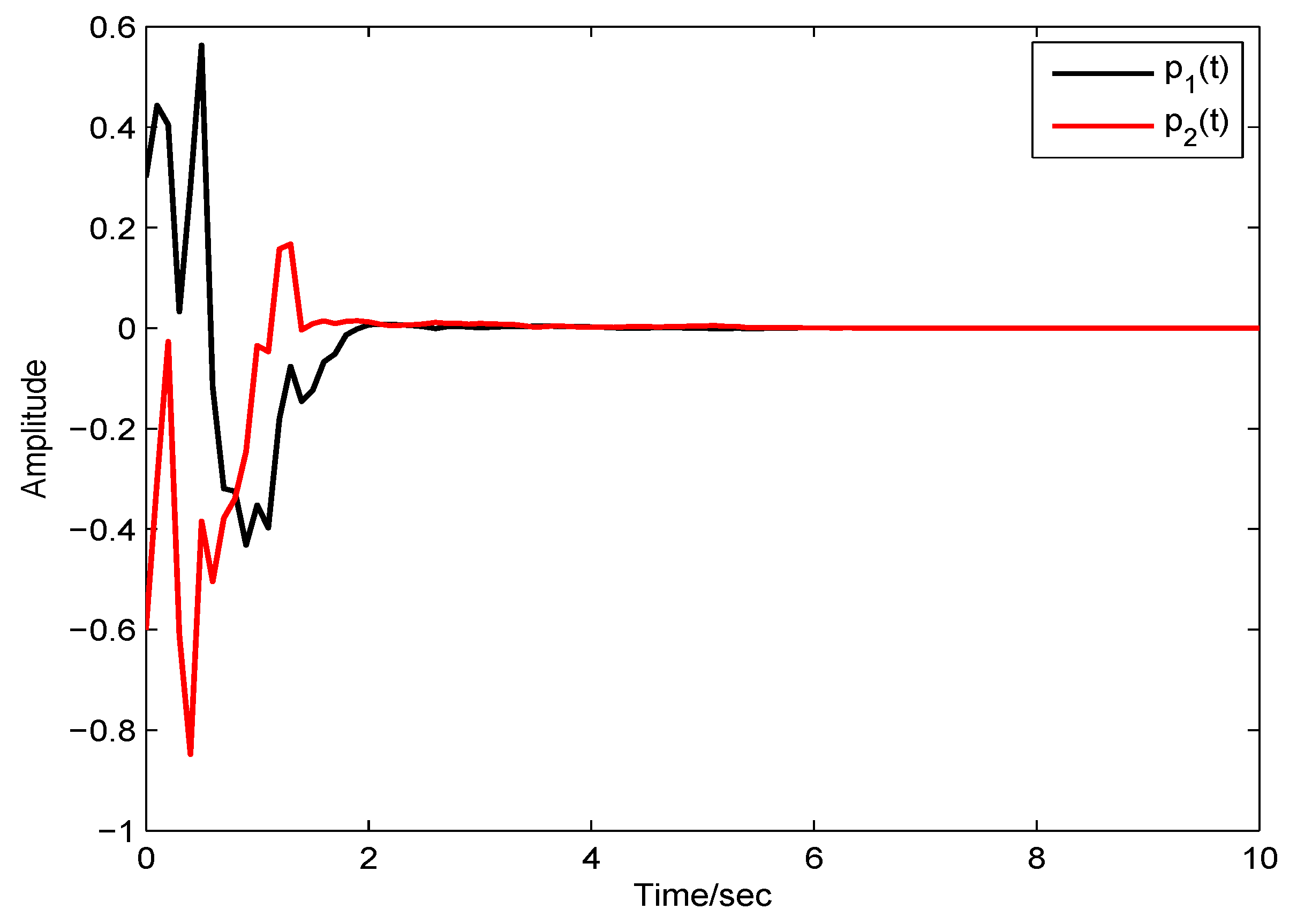
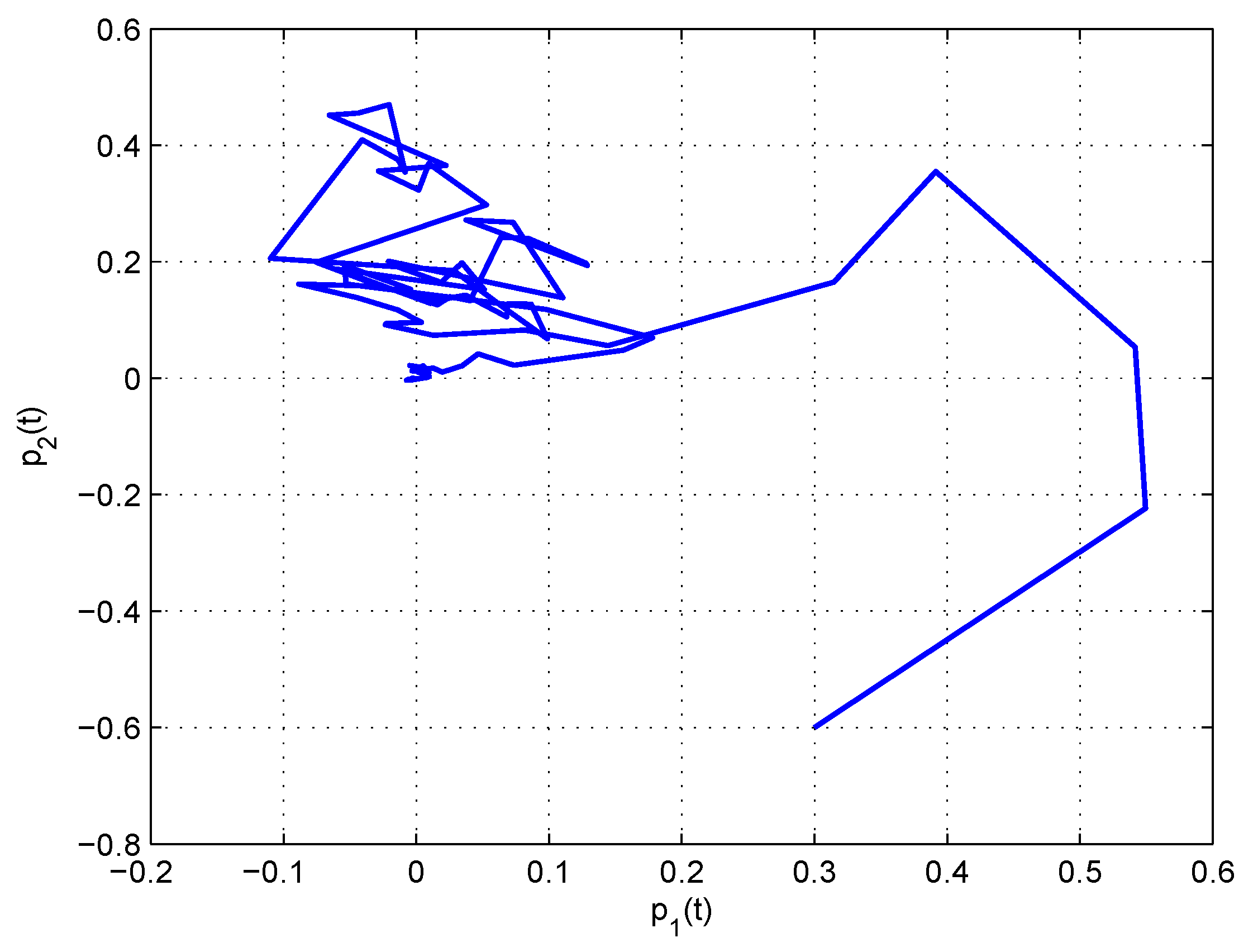
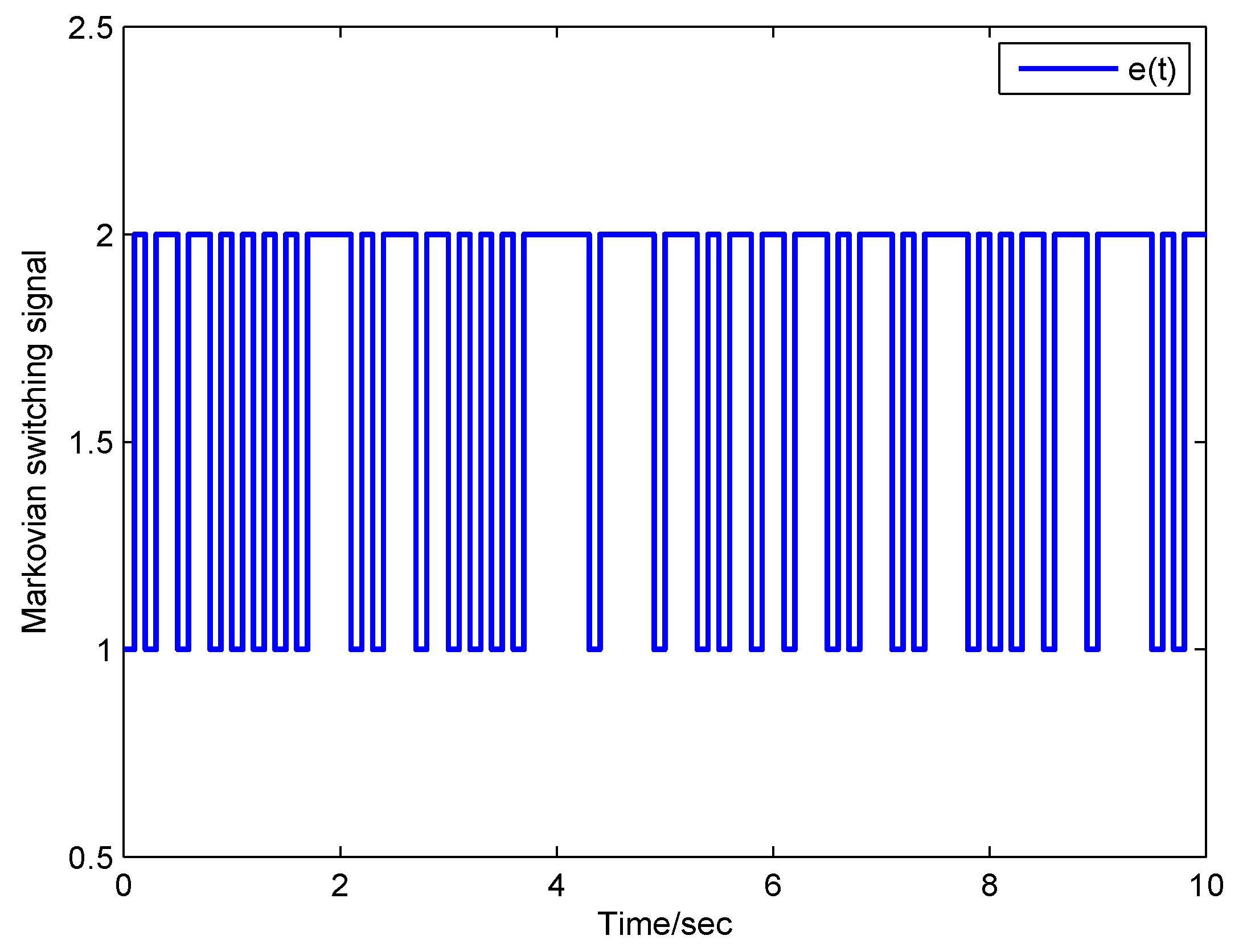
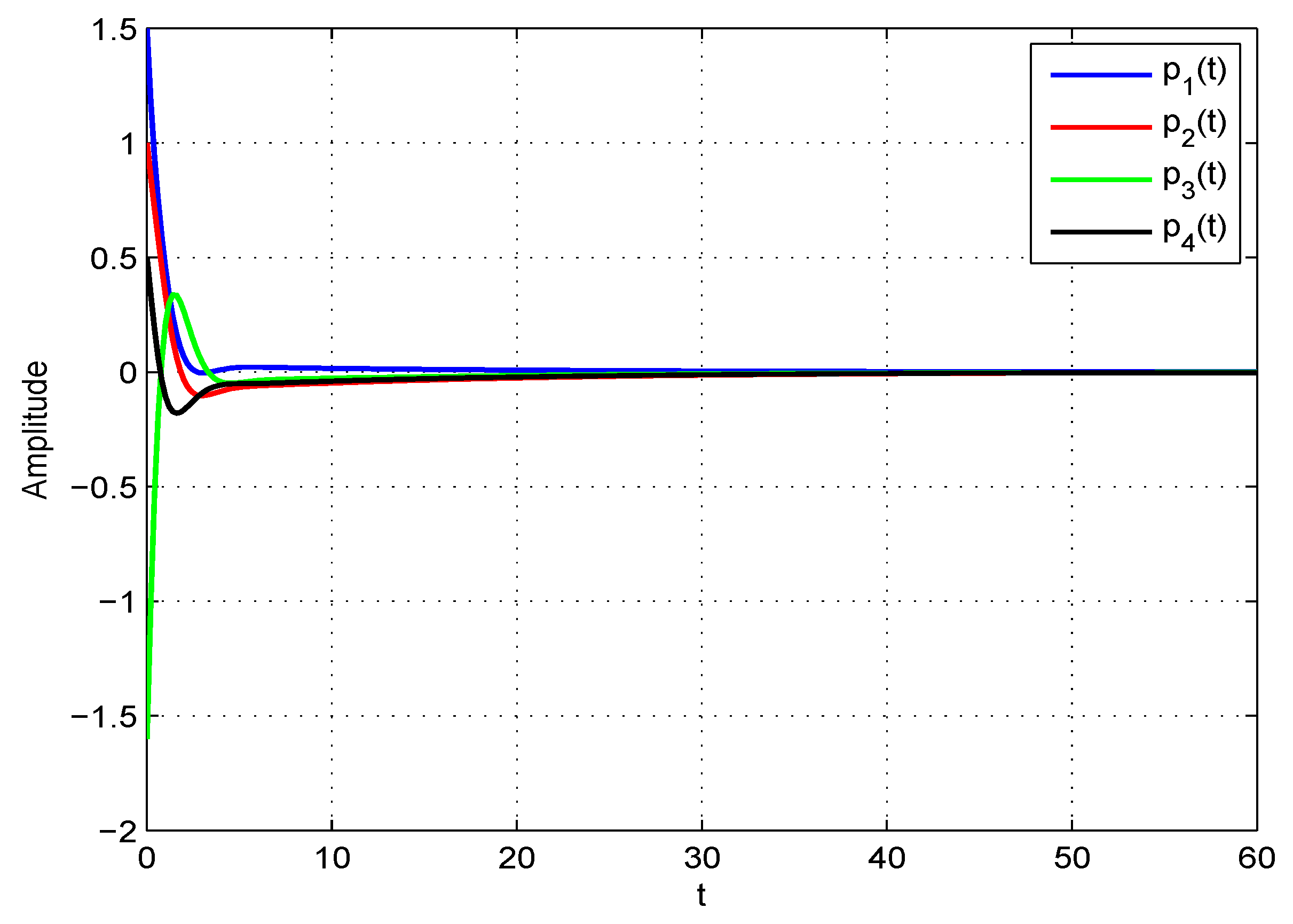
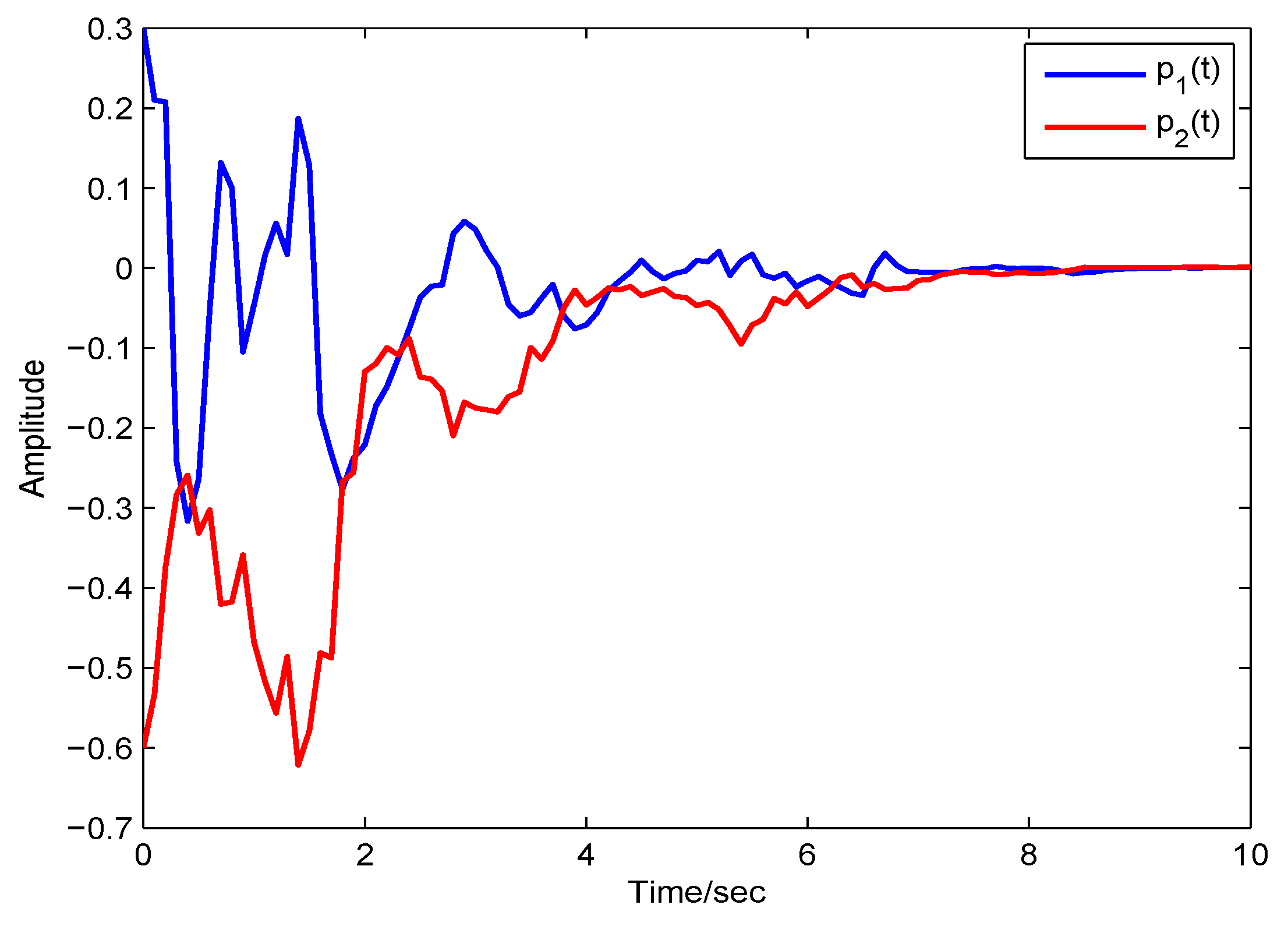
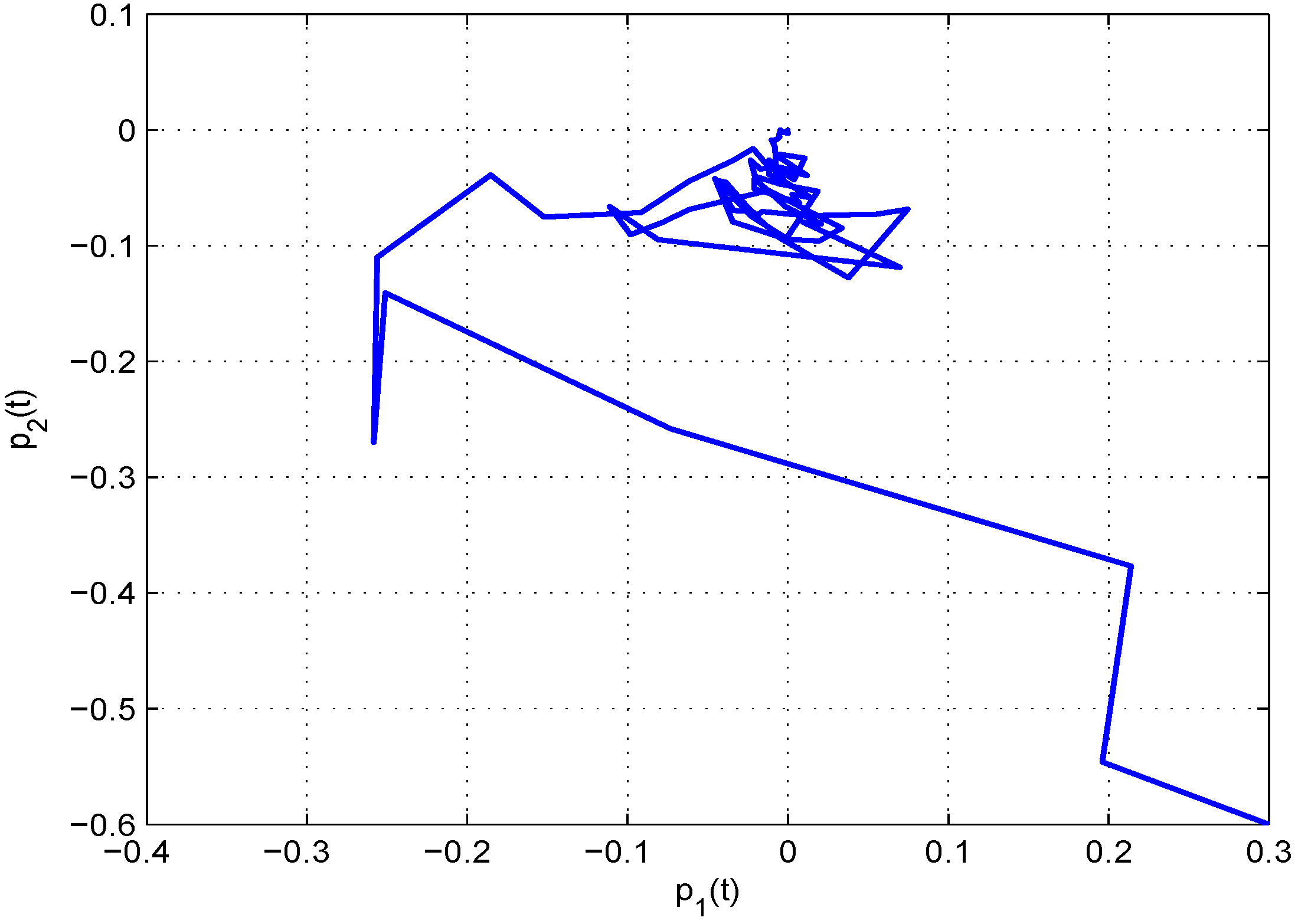
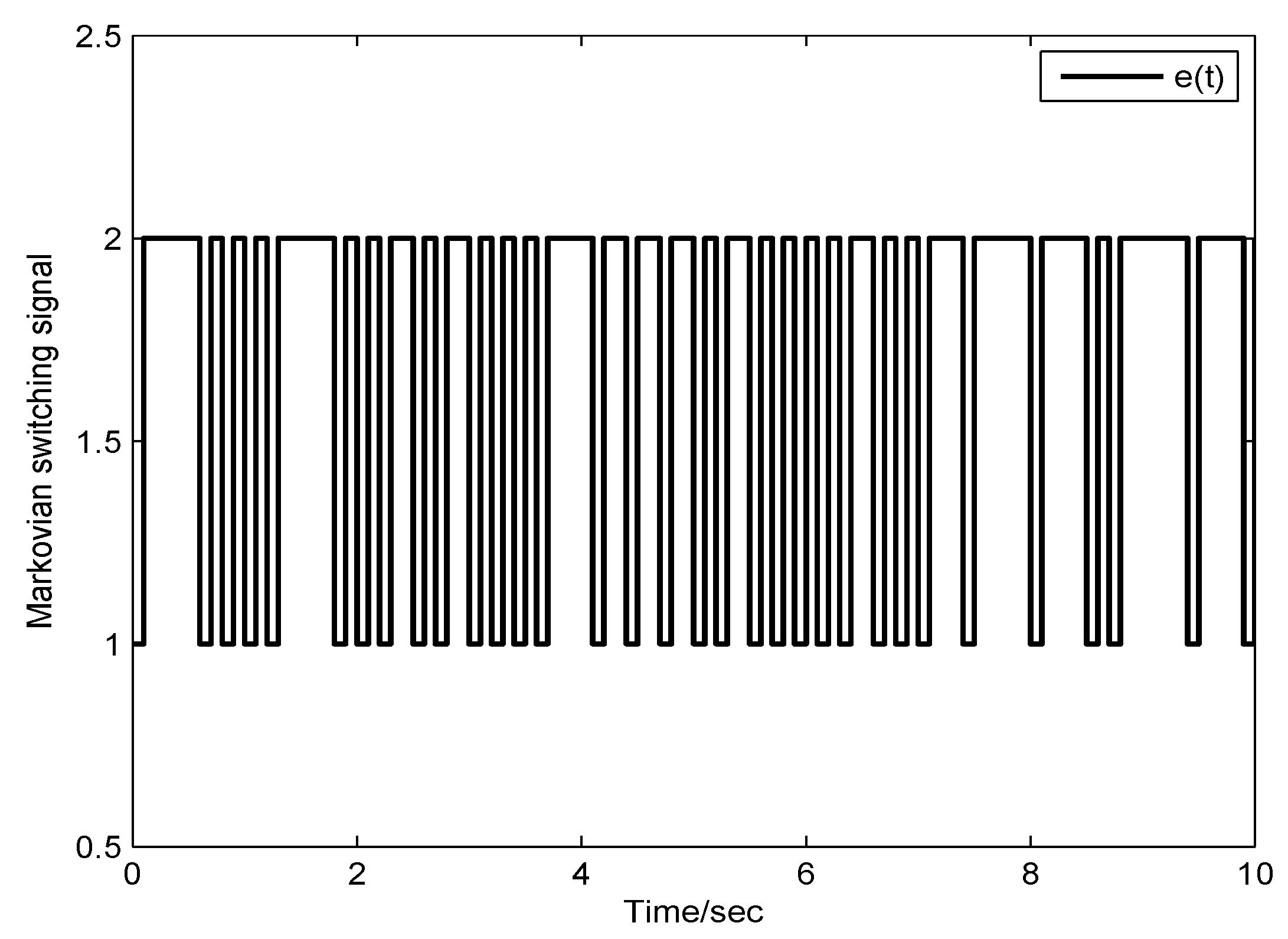
4. Simulation Studies

The usefulness of the obtain results is evaluated using three simulated examples.

Example 1.

Consider Model (6) with respect to both modes below:

$$\begin{array}{cc}\hfill {\mathbf{D}}_1=& \left[\begin{array}{cc}2.2& 0\\ 0& 1.8\end{array}\right],{\mathbf{A}}_1=\left[\begin{array}{cc}0.3& 0.2\\ 0.3& -0.2\end{array}\right],{\mathbf{B}}_1=\left[\begin{array}{cc}0.2& -0.3\\ 0.4& 0.2\end{array}\right],\hfill \\ \hfill {\mathbf{W}}_1=& \left[\begin{array}{cc}1& 0\\ 0& 1\end{array}\right],{\mathbf{L}}_{11}=\left[\begin{array}{cc}0.22& 0\\ 0& 0.22\end{array}\right],{\mathbf{L}}_{21}=\left[\begin{array}{cc}0.18& 0\\ 0& 0.18\end{array}\right],\hfill \\ \hfill {\mathbf{D}}_2=& \left[\begin{array}{cc}1.4& 0\\ 0& 2\end{array}\right],{\mathbf{A}}_2=\left[\begin{array}{cc}0.3& 0.5\\ -0.2& 0.1\end{array}\right],{\mathbf{B}}_2=\left[\begin{array}{cc}0.3& 0.2\\ -0.3& 0.5\end{array}\right],\hfill \\ \hfill {\mathbf{W}}_2=& \left[\begin{array}{cc}1& 0\\ 0& 1\end{array}\right],{\mathbf{L}}_{12}=\left[\begin{array}{cc}0.20& 0\\ 0& 0.20\end{array}\right],{\mathbf{L}}_{22}=\left[\begin{array}{cc}0.12& 0\\ 0& 0.12\end{array}\right].\hfill \end{array}$$

Moreover, we take,

$$\begin{array}{c}\hfill \mathcal{Q}=\left[\begin{array}{cc}-7& 0\\ 0& -7\end{array}\right],\mathcal{S}=\left[\begin{array}{cc}0.1& -0.1\\ -0.1& 0.5\end{array}\right],\mathcal{R}=\left[\begin{array}{cc}12& 0\\ 0& 12\end{array}\right].\end{array}$$

Let $\mathsf{\Pi }=\left[\begin{array}{cc}-3& 3\\ 2& -2\end{array}\right]$ and $r\left(t\right)=0.2+0.1sint$, which satisfies $r=0.3,\mu =0.2$. Furthermore, choose $g_i\left(p_i\left(t\right)\right)=tanh\left(p_i\left(t\right)\right),i=1,2$. As a result, we have ${\Delta }_1=0,{\Delta }_2=\mathbf{I}$. In addition, from (32), we have ${\mathbf{K}}_1=0,{\mathbf{K}}_2=-0.5\mathbf{I}$. We show that LMIs (14) and (15) are valid using MATLAB. The initial values are chosen as $p\left(0\right)={[0.3,-0.6]}^T$. As such, the following simulation results can be obtained by taking $u\left(t\right)=0.01e^{-t}sin\left(0.02t\right)t>0$ with respect to the model in (6). Figure 1 shows that time responses of Model (6). The state transient response of Model (6) is displayed in Figure 2. Figure 3 describes the Markovian switching signal.

Example 2.

We consider Model (46) subject to $x=1$ along with the following parameters:

$$\begin{array}{cc}\hfill \mathbf{A}=& \left[\begin{array}{cccc}-0.0373& 0.4852& -0.3351& 0.2336\\ -1.6033& 0.5988& -0.3224& 1.2352\\ 0.3394& -0.0860& -0.3894& -0.5785\\ -0.1311& 0.3253& -0.9534& -0.5015\end{array}\right],\mathbf{B}=\left[\begin{array}{cccc}0.8674& -1.2405& -0.5325& 0.0220\\ 0.0474& -0.9164& 0.0360& 0.9816\\ 1.8495& 2.6117& -0.3788& 0.8428\\ -2.0413& 0.5179& 1.1734& -0.2775\end{array}\right],\hfill \\ \hfill \mathbf{D}=& diag\{1.2769,0.6231,0.9230,0.4480\},\mathbf{W}=diag\{1,1,1,1\}.\hfill \end{array}$$

This simulation study facilitates the comparison pertaining to the criteria in [11,12,13]. The neuron activation function is chosen as $g_i\left(p_i\left(t\right)\right)=0.2tanh\left(p_i\left(t\right)\right),i=1,2,3,4$. As a result, we have ${\Delta }_1=0,{\Delta }_2=diag\{0.1137,0.1279,0.7994,0.2368\}$. In addition, from (32), we have ${\mathbf{K}}_1=0,{\mathbf{K}}_2=diag\{-\frac{0.1137}{2},-\frac{0.1279}{2},-\frac{0.7994}{2},-\frac{0.2368}{2}\}$. We show that LMI (47) is valid using MATLAB. For various setting of μ, the maximum permissible delay limit r is listed in

Table 1. The maximum permissible delay limit r with different μ settings.

Methods	$\mathit{\mu }$	0.1	0.5	0.9
[11]	r	3.8739	2.7821	2.3279
[12]	r	4.1903	3.0779	2.8268
[13]	r	4.1919	3.0790	2.8271
Corollary 4	r	4.1920	3.0791	2.8272

. It is evident that the obtained results in this paper show less conservatism than those in [11,12,13]. For the simulation purpose, we used $r\left(t\right)=2.6272+0.2sint$, which satisfies $r=2.8272$. The following simulation results for the initial condition $p\left(0\right)={[1.5,1,-1.6,0.5]}^T$. The time responses of the state variables $p_1\left(t\right),p_2\left(t\right),p_3\left(t\right),p_4\left(t\right)$ of Model (46) are depicted in Figure 4. According to Corollary 4, the GNN (46) is globally asymptotically stable.

Remark 7.

In regard to computational complexity analysis, the main governing factor is the maximum number of decision variables in the LMIs. The use of delay augmented LKFs [32] and the free-matrix based methods [33] leads to an increase in the number of decision variables. As such, the computational load and complexity increase with respect to the increase in the number of delay subintervals. To address this problem, we chose suitable LKFs and exploited new inequalities with tighter bounds, in order to derive simplified LMI based sufficient conditions and yield less conservative results as compared with those in [11,12,13]. In addition to less conservatism, our results required a lower computational load, because we did not adopt any free-matrix based methods or delay-decomposing methods in our theoretical analysis. In [13], enhanced stability criteria pertaining to GNN model were derived with free-matrix based methods coupled with augmented LKFs, which resulted in many decision variables, i.e., $82n^2+5n$. Comparatively, we only required on $18n^2+5n$ decision various in our results. Therefore, it was evident that our results were less conservative with a smaller computational load.

Example 3.

Consider Model (48) with respect to both modes below.

$$\begin{array}{cc}\hfill {\mathbf{D}}_1=& \left[\begin{array}{cc}2.2& 0\\ 0& 1.8\end{array}\right],{\mathbf{A}}_1=\left[\begin{array}{cc}0.3& 0.2\\ 0.3& -0.2\end{array}\right],{\mathbf{B}}_1=\left[\begin{array}{cc}0.2& -0.3\\ 0.4& 0.2\end{array}\right],{\mathbf{W}}_1=\left[\begin{array}{cc}1& 0\\ 0& 1\end{array}\right],\hfill \\ \hfill {\mathbf{L}}_{11}=& \left[\begin{array}{cc}0.22& 0\\ 0& 0.22\end{array}\right],{\mathbf{L}}_{21}=\left[\begin{array}{cc}0.18& 0\\ 0& 0.18\end{array}\right],{\mathbf{M}}_1=\left[\begin{array}{cc}0.2& 0\\ 0& 0.2\end{array}\right],\hfill \\ \hfill {\mathbf{N}}_{11}=& \left[\begin{array}{cc}0.3& 0\\ 0& 0.3\end{array}\right],{\mathbf{N}}_{21}=\left[\begin{array}{cc}0.2& 0\\ 0& 0.2\end{array}\right],{\mathbf{N}}_{31}=\left[\begin{array}{cc}0.1& 0\\ 0& 0.1\end{array}\right],\hfill \\ \hfill {\mathbf{D}}_2=& \left[\begin{array}{cc}1.4& 0\\ 0& 2\end{array}\right],{\mathbf{A}}_2=\left[\begin{array}{cc}0.3& 0.5\\ -0.2& 0.1\end{array}\right],{\mathbf{B}}_2=\left[\begin{array}{cc}0.3& 0.2\\ -0.3& 0.5\end{array}\right],{\mathbf{W}}_2=\left[\begin{array}{cc}1& 0\\ 0& 1\end{array}\right],\hfill \\ \hfill {\mathbf{L}}_{12}=& \left[\begin{array}{cc}0.20& 0\\ 0& 0.20\end{array}\right],{\mathbf{L}}_{22}=\left[\begin{array}{cc}0.12& 0\\ 0& 0.12\end{array}\right],{\mathbf{M}}_2=\left[\begin{array}{cc}0.2& 0\\ 0& 0.2\end{array}\right],\hfill \\ \hfill {\mathbf{N}}_{12}=& \left[\begin{array}{cc}0.3& 0\\ 0& 0.3\end{array}\right],{\mathbf{N}}_{22}=\left[\begin{array}{cc}0.2& 0\\ 0& 0.2\end{array}\right],{\mathbf{N}}_{32}=\left[\begin{array}{cc}0.1& 0\\ 0& 0.1\end{array}\right],\hfill \end{array}$$

Moreover, we take,

$$\begin{array}{c}\hfill \mathcal{Q}=\left[\begin{array}{cc}-1& 0\\ 0& -1\end{array}\right],\mathcal{S}=\left[\begin{array}{cc}1& 0\\ 1& 1\end{array}\right],\mathcal{R}=\left[\begin{array}{cc}3& 0\\ 0& 3\end{array}\right].\end{array}$$

Let $\mathsf{\Pi }=\left[\begin{array}{cc}-3& 3\\ 2& -2\end{array}\right]$ and $r\left(t\right)=0.2+0.1sint$, which satisfies $r=0.3,\mu =0.2$. Furthermore, choose $g_i\left(p_i\left(t\right)\right)=tanh\left(p_i\left(t\right)\right),i=1,2$, and we have ${\Delta }_1=0,{\Delta }_2=\mathbf{I}$. In addition, from (32), we have ${\mathbf{K}}_1=0,{\mathbf{K}}_2=-0.5\mathbf{I}$. We show that LMIs (50) and (51) are valid using MATLAB. Under the the initial values $p\left(0\right)={[0.3,-0.6]}^T$, the following results can be obtained by taking $u\left(t\right)=0.01e^{-t}sin\left(0.02t\right)t>0$. For Model (48), the time responses with respect to variables $p_1\left(t\right),p_2\left(t\right)$ are given in Figure 5. Figure 6 describes the transient responses of variables $p_1\left(t\right),p_2\left(t\right)$. The Markovian switching signals are depicted in Figure 7.

5. Conclusions

In this article, we analyzed the robust dissipativity of USGNN models incorporating MJPs and time-varying delays. Our analyses covered a more general form of USGNN models, which took both stochastic effects and parameter uncertainties into consideration. To facilitate our analyses, we formulated appropriate LKFs along with effective integral inequalities and sector bound conditions. As such, we derived several simplified LMI based sufficient conditions. The corresponding feasible solutions were validated using MATLAB. We also ascertained the usefulness of our results with three simulation examples.

For further research, we will analyze other types of stochastic NN models with the proposed method. The stability and synchronization analyses of stochastic fuzzy NN models, coupled stochastic NN models, fractional-order NN models, and memristor based stochastic NN models can be conducted. Applications of the resulting NN models to various control and engineering problems will also be examined.

References

1. Cao, J. Global asymptotic stability of neural networks with transmission delays. Int. J. Syst. Sci. 2000, 31, 1313–1316. [Google Scholar] [CrossRef]
2. Arik, S. An analysis of global asymptotic stability of delayed cellular neural networks. IEEE Trans. Neural Netw. 2012, 13, 1239–1242. [Google Scholar] [CrossRef] [PubMed]
3. Zhao, Z.; Song, Q.; He, S. Passivity analysis of stochastic neural networks with time-varying delays and leakage delay. Neurocomputing 2014, 125, 22–27. [Google Scholar] [CrossRef]
4. Wei, H.; Li, R.; Chen, C. State estimation for memristor-based neural networks with time-varying delays. Int. J. Mach. Learn. Cybern. 2015, 6, 213–225. [Google Scholar] [CrossRef]
5. Huang, H.; Huang, T.; Cao, Y. Reduced-order filtering of delayed static neural networks with Markovian jumping parameters. IEEE Trans. Neural Netw. Learn. Syst. 2018, 29, 5606–5618. [Google Scholar] [CrossRef] [PubMed]
6. Arunkumar, A.; Sakthivel, R.; Mathiyalagan, K.; Park, J.H. Robust stochastic stability of discrete-time fuzzy Markovian jump neural networks. ISA Trans. 2014, 53, 1006–1014. [Google Scholar] [CrossRef]
7. Chen, Y.; Wang, Z.; Liu, Y.; Alsaadi, F.E. Stochastic stability for distributed delay neural networks via augmented Lyapunov–Krasovskii functionals. Appl. Math. Comput. 2018, 338, 869–881. [Google Scholar] [CrossRef]
8. Chen, G.; Xia, J.; Zhuang, G. Delay-dependent stability and dissipativity analysis of generalized neural networks with Markovian jump parameters and two delay components. J. Frankl. Inst. 2016, 353, 2137–2158. [Google Scholar] [CrossRef]
9. Samidurai, R.; Manivannan, R.; Ahn, C.K.; Karimi, H.R. New criteria for stability of generalized neural networks including Markov jump parameters and additive time delays. IEEE Trans. Syst. Man Cybern. Syst. 2018, 48, 485–499. [Google Scholar] [CrossRef]
10. Jiao, S.; Shen, H.; Wei, Y.; Huang, X.; Wang, Z. Further results on dissipativity and stability analysis of Markov jump generalized neural networks with time-varying interval delays. Appl. Math. Comput. 2018, 336, 338–350. [Google Scholar] [CrossRef]
11. Zhang, C.K.; He, Y.; Jiang, L.; Wu, Q.H.; Wu, M. Delay-dependent stability criteria for generalized neural networks with two delay components. IEEE Trans. Neural Netw. Learn. Syst. 2014, 25, 1263–1276. [Google Scholar] [CrossRef]
12. Zeng, H.B.; He, Y.; Wu, M.; Xiao, S. Stability analysis of generalized neural networks with time-varying delays via a new integral inequality. Neurocomputing 2015, 161, 148–154. [Google Scholar] [CrossRef]
13. Wang, B.; Yan, J.; Cheng, J.; Zhong, S. New criteria of stability analysis for generalized neural networks subject to time-varying delayed signals. Appl. Math. Comput. 2017, 314, 322–333. [Google Scholar] [CrossRef]
14. Sriraman, R.; Cao, Y.; Samidurai, R. Global asymptotic stability of stochastic complex-valued neural networks with probabilistic time-varying delays. Math. Comput. Simulat. 2020, 171, 103–118. [Google Scholar] [CrossRef]
15. Wang, C.; Shen, Y. Delay-dependent non-fragile robust stabilization and H control of uncertain stochastic systems with time-varying delay and nonlinearity. J. Frankl. Inst. 2011, 348, 2174–2190. [Google Scholar] [CrossRef]
16. Samidurai, R.; Sriraman, R. Robust dissipativity analysis for uncertain neural networks with additive time-varying delays and general activation functions. Math. Comput. Simulat. 2019, 155, 201–216. [Google Scholar] [CrossRef]
17. Boukas, E.K.; Liu, Z.K.; Liu, G.X. Delay-dependent robust stability and H control of jump linear systems with time-delay. Int. J. Control 2010, 74, 329–340. [Google Scholar] [CrossRef]
18. Cao, Y.Y.; Lam, J.; Hu, L.S. Delay-dependent stochastic stability and H analysis for time-delay systems with Markovian jumping parameters. J. Frankl. Inst. 2013, 340, 423–434. [Google Scholar] [CrossRef]
19. Zhu, Q.; Cao, J. Exponential stability of stochastic neural networks with both Markovian jump parameters and mixed time delays. IEEE Trans. Syst. Man Cybern. Part B 2011, 41, 341–353. [Google Scholar]
20. Tan, H.; Hua, M.; Chen, J.; Fei, J. Stability analysis of stochastic Markovian switching static neural networks with asynchronous mode-dependent delays. Neurocomputing 2015, 151, 864–872. [Google Scholar] [CrossRef]
21. Zhu, S.; Shen, M.; Lim, C.C. Robust input-to-state stability of neural networks with Markovian switching in presence of random disturbances or time delays. Neurocomputing 2017, 249, 245–252. [Google Scholar] [CrossRef]
22. Blythe, S.; Mao, X.; Liao, X. Stability of stochastic delay neural networks. J. Frankl. Inst. 2001, 338, 481–495. [Google Scholar] [CrossRef]
23. Chen, Y.; Zheng, W. Stability analysis of time-delay neural networks subject to stochastic perturbations. IEEE Trans. Cybern. 2013, 43, 2122–2134. [Google Scholar] [CrossRef] [PubMed]
24. Yang, R.; Gao, H.; Shi, P. Novel robust stability criteria for stochastic Hopfield neural networks with time delays. IEEE Trans. Syst. Man Cybern. Part B 2009, 39, 467–474. [Google Scholar] [CrossRef] [PubMed]
25. Zhu, S.; Shen, Y. Passivity analysis of stochastic delayed neural networks with Markovian switching. Neurocomputing 2011, 74, 1754–1761. [Google Scholar] [CrossRef]
26. Cao, Y.; Samidurai, R.; Sriraman, R. Stability and dissipativity analysis for neutral type stochastic Markovian jump static neural networks with time delays. J. Artif. Int. Soft Comput. Res. 2019, 9, 189–204. [Google Scholar] [CrossRef] [Green Version]
27. Liu, G.; Yang, S.X.; Chai, Y.; Feng, W.; Fu, W. Robust stability criteria for uncertain stochastic neural networks of neutral-type with interval time-varying delays. Neural Comput. Appl. 2013, 22, 349–359. [Google Scholar] [CrossRef]
28. Pradeep, C.; Chandrasekar, A.; Murugesu, M.; Rakkiyappan, R. Robust stability analysis of stochastic neural networks with Markovian jumping parameters and probabilistic time-varying delays. Complexity 2014, 21, 59–72. [Google Scholar] [CrossRef]
29. Sakthivel, R.; Arunkumar, A.; Mathiyalagan, K.; Marshal Anthoni, S. Robust passivity analysis of fuzzy Cohen-Grossberg BAM neural networks with time-varying delays. Appl. Math. Comput. 2011, 275, 213–228. [Google Scholar] [CrossRef]
30. Kwon, O.M.; Lee, S.M.; Park, J.H. Improved delay-dependent exponential stability for uncertain stochastic neural networks with time-varying delays. Phys. Lett. A 2010, 374, 1232–1241. [Google Scholar] [CrossRef]
31. Muthukumar, P.; Subramanian, K.; Lakshmanan, S. Robust finite time stabilization analysis for uncertain neural networks with leakage delay and probabilistic time-varying delays. J. Frankl. Inst. 2016, 353, 4091–4113. [Google Scholar] [CrossRef]
32. Lee, C.H.; Lee, S.H.; Park, M.J.; Kwon, O.M. Stability and stabilization criteria for sampled-data control system via augmented Lyapunov–Krasovskii functionals. Int. J. Control. Autom. Syst. 2018, 16, 2290–2302. [Google Scholar] [CrossRef]
33. Park, M.J.; Lee, S.H.; Kwon, O.M.; Ryu, J.H. Enhanced stability criteria of neural networks with time-varying delays via a generalized free-weighting matrix integral inequality. J. Frankl. Inst. 2018, 355, 6531–6548. [Google Scholar] [CrossRef]
34. Willems, J.C. Dissipative dynamical systems part I: General theory. Arch. Ration. Mech. Anal. 1972, 45, 321–351. [Google Scholar] [CrossRef]
35. Hill, D.L.; Moylan, P.J. Dissipative dynamical systems: Basic input-output and state properties. J. Frankl. Inst. 1980, 309, 327–357. [Google Scholar] [CrossRef]
36. Wu, Z.G.; Park, J.H.; Su, H.; Chu, J. Robust dissipativity analysis of neural networks with time-varying delay and randomly occurring uncertainties. Nonlinear Dyn. 2012, 69, 1323–1332. [Google Scholar] [CrossRef]
37. Liao, X.; Wang, J. Global dissipativity of continuous-time recurrent neural networks with time delay. Phys. Rev. E 2013, 68, 016118. [Google Scholar] [CrossRef]
38. Song, Q.; Zhao, Z. Global dissipativity of neural networks with both variable and unbounded delays. Chaos Solitons Fract. 2005, 25, 393–401. [Google Scholar] [CrossRef]
39. Feng, Z.; Lam, J. Stability and dissipativity analysis of distributed delay cellular neural networks. IEEE Trans. Neural Netw. 2011, 22, 976–981. [Google Scholar] [CrossRef]
40. Raja, R.; Raja, U.K.; Samidurai, R.; Leelamani, A. Dissipativity of discrete-time BAM stochastic neural networks with Markovian switching and impulses. J. Frankl. Inst. 2013, 350, 3217–3247. [Google Scholar] [CrossRef]
41. Zeng, H.B.; Park, J.H.; Zhang, C.F.; Wang, W. Stability and dissipativity analysis of static neural networks with interval time-varying delay. J. Frankl. Inst. 2015, 352, 1284–1295. [Google Scholar] [CrossRef]
42. Cao, J.; Yuan, K.; Ho, D.W.C.; Lam, J. Global point dissipativity of neural networks with mixed time-varying delays. Chaos 2006, 16, 013105. [Google Scholar] [CrossRef] [PubMed] [Green Version]
43. Zhang, L.; He, L.; Song, Y. New results on stability analysis of delayed systems derived from extended Wirtingers integral inequality. Neurocomputing 2018, 283, 98–106. [Google Scholar] [CrossRef]
44. Samidurai, R.; Sriraman, R. Non-fragile sampled-data stabilization analysis for linear systems with probabilistic time-varying delays. J. Frankl. Inst. 2019, 356, 4335–4357. [Google Scholar] [CrossRef]
45. Gu, K.; Kharitonov, V.L.; Chen, J. Stability of Time-Delay Systems; Birkhäuser: Boston, MA, USA, 2003. [Google Scholar]
46. Zhu, Q.; Cao, J. Robust exponential stability of Markovian jump impulsive stochastic Cohen-Grossberg neural networks with mixed time delays. IEEE Trans. Neural Netw. 2010, 21, 1314–1325. [Google Scholar]
Figure 1. Time responses of the state variables p 1 ( t ) , p 2 ( t ) with respect to Model (6) in Example 1.
Symmetry 12 01035 g001
Figure 2. Transient responses of the state variables p 1 ( t ) , p 2 ( t ) with respect to Model (6) in Example 1.
Symmetry 12 01035 g002
Figure 3. The Markovian switching signal e ( t ) in Example 1.
Symmetry 12 01035 g003
Figure 4. Time responses of the state variables p 1 ( t ) , p 2 ( t ) , p 3 ( t ) , p 4 ( t ) with respect to Model (46) in Example 2.
Symmetry 12 01035 g004
Figure 5. Time responses of the state variables p 1 ( t ) , p 2 ( t ) with respect to Model (48) in Example 3.
Symmetry 12 01035 g005
Figure 6. Transient responses of the state variables p 1 ( t ) , p 2 ( t ) with respect to Model (48) in Example 3.
Symmetry 12 01035 g006
Figure 7. The Markovian switching signal e ( t ) in Example 3.
Symmetry 12 01035 g007