Simple Solutions of Lattice Sums for Electric Fields Due to Infinitely Many Parallel Line Charges

Abstract

We present surprisingly simple closed-form solutions for electric fields and electric potentials at arbitrary position $\left(x,y\right)$ within a plane crossed by infinitely long line charges at regularly repeating positions using angular or elliptic functions with complex arguments. The lattice sums for the electric-field components and the electric potentials could be exactly solved, and the duality symmetry of trigonometric and lemniscate functions occurred in some solutions. The results may have relevance in calculating field configurations with rectangular boundary conditions. Several series related to Gauss’s constant are presented, established either as corollary results or via parallel investigations conducted in the spirit of experimental mathematics.

1. Introduction

The study of lattice sums has a long history. They are frequently encountered when studying physical and chemical systems (e.g., [1] and references therein). In the present work, we targeted lattice sums arising from the consideration of electric fields and electric potentials set up by the crossing of infinitely many and infinitely long line charges through horizontally and/or vertically equidistant co-ordinates of the Gaussian plane. The line charges had the same charge density magnitude, while their signs were set according to the specific scenario we envisioned. Problems of a similar nature, such as wire-grid problems, were extensively studied in the past; see e.g., K. T. McDonald’s Notes on Electrostatic Wire Grids [2] where in turn a reference is made to Maxwell’s famous book A Treatise on Electricity and Magnetism. Related results may have applications beyond electrostatics. For instance, in solid-state physics, stress fields generated by screw dislocations seem to be mathematically analogous to the electric field due to line charges (see Section 2.8 of [3] and references therein).

Our study was motivated by an initial (and accidental) discovery (see Equation (2) in Section 2) that pointed to a possible solution for electric-field components in a certain line-charge arrangement in terms of lemniscate functions. After establishing a closed-form solution for a related but more general lattice sum, we searched for this identity, browsing through [1,4,5,6] and other printed and online sources accessible to us, without finding a match. This led us to examine a variety of line-charge schemes.

We established closed-form expressions for the electric field and the electric potential at an arbitrary position $\left(x, y\right)$ for different line-charge arrangements. The closed-form solutions of encountered double sums involved the lemniscate constant (L = 2.6220575…), and the sine and/or cosine lemniscate functions (sl and cl, respectively). It was no wonder that elliptic functions, with double periodicity, appeared in the solution of double lattice series, but of special interest in our case was the duality, a certain kind of similarity between lemniscate functions and their trigonometric counterparts. For definitions and properties of lemniscate functions, see, e.g., [7,8,9] or online sources such as [10]. Here we specify two fast-converging series useful for the numeric evaluation of sl and cl [11]:

$$\mathbf{sl}\left(z\right)=\frac{4\pi }{L}\sin \left[\frac{\pi z}{L}\right]{\displaystyle \sum }_{k=0}^s\frac{{\left(-1\right)}^k\sinh \left[\left(2k+1\right)\frac{\pi }{2}\right]}{\cosh \left[\left(2k+1\right)\pi \right]+\cos \left[\frac{2\pi z}{L}\right]}$$

(1a)

$$\mathbf{cl}\left(z\right)=\frac{4\pi }{L}\cos \left[\frac{\pi z}{L}\right]{\displaystyle \sum }_{k=0}^s\frac{{\left(-1\right)}^k\sinh \left[\left(2k+1\right)\frac{\pi }{2}\right]}{\cosh \left[\left(2k+1\right)\pi \right]-\cos \left[\frac{2\pi z}{L}\right]}$$

(1b)

The precision of the approximation varies with ${10}^{-3s/2}$ as seen by comparing numerical results to sl and cl expressed as Jacobian elliptic functions (see e.g., [7,10]). As an example, with $z=L/2$, for which we know that $\mathbf{sl}\left(z\right)=1$, computation of the right-hand side of Equation (1a) with $s=5$ returns the result 0.99999999378… We also calculated the first five nonzero Taylor expansion coefficients of the sl function (found in the Online Encyclopedia of Integer Sequences [12] as sequence A104203) using Equation (1a) with s = 4 as: {1.000000172; −11.99999964; 3024.000001; −4,390,848; 21,224,560,896}. A corresponding result was obtained for the cl function. Other series expansions for the cl function may be found in [13], and these may also be used for sl via the property $sl\left(z\right)=cl\left(z-L/2\right),$ where z is any complex number.

Section 2 gives a brief account of how we arrived at the closed-form results. In Section 3 we introduce the considered cases as well as their solutions (electric-field components, electric potential). Section 4 discusses earlier works, that we came across, highlights duality, presents corollary results related to Gauss’s constant, and also addresses applications to particle detectors with long charged wires being in the middle of conducting surfaces. Section 5 presents a conclusion.

2. Investigation Method

Our study was initiated by the coincidental finding that the lattice sum

$${\displaystyle \sum }_{m,n=-\infty }^{\infty }{\left(-1\right)}^{m+n}\frac{1/2-m}{{\left(1/2-m\right)}^2+n^2}=L=\sqrt{{\pi }^3}/\left(\sqrt{2}\mathsf{\Gamma }{\left(\frac{3}{4}\right)}^2\right)$$

(2)

where L = 2.6220575… is the lemniscate constant, and $\mathsf{\Gamma }{(}_{-})$ stands for the gamma function. This result (the key identity) was tested in Mathematica [14] via symbolic summing over one index, then numerically summing the resulting hyperbolic cosecant over the second index, and it was found to hold to better than 6000 digits thanks to the high-precision capabilities of Mathematica. This does not count as a mathematical proof in the strict sense, but we took the identity given in Equation (2) as valid, at least within the verified precision. In the same manner, we relied on quite strict numerical verification when the difficulty of symbolic calculation exceeded our capabilities. Equation (2) can be read as the solution for a special case of an electrostatic problem, where comparable series appear as will be explained next.

We work in the CGS-Gaussian system of units. A single line charge produces an electric field in a radial direction, inward or outward, with a magnitude determined by the product of the charge times twice the reciprocal of the distance. The electrostatic potential of an arrangement of line charges in a plane perpendicular to the wires is usually calculated by superposition as an explicit sum of the potentials due to every single line charge. Formally:

$$U\left(x,y\right)=-2{\displaystyle \sum }_k{\lambda }_k\log \left(\left|{\mathit{r}}_k\left(x,y\right)\right|\right)-U\left(x_{ref},y_{ref}\right)$$

(3)

where ${\lambda }_k$ identifies the single line-charge density, and ${\mathit{r}}_k$ denotes the vectorial distance measured from the position of the wire to a point $\left(x, y\right)$ in the plane (e.g., [15]). The reference point marks a location where the potential is set to zero. The relation of Equation (2) to electric field configurations of certain distributions of line charges becomes evident if we consider the electric fields in Cartesian co-ordinates. The electric field of a potential due to several distributed line charges in the $\left(x, y\right)$-plane is given by the negative gradient of Equation (3). The $x$-component of the field at $\left(x,y\right)$ for instance then reads for charges of equal magnitude:

$$E_x\left(x,y\right)=2\lambda {\partial }_x\left({\displaystyle \sum }_k\log \sqrt{{\left(x-x_{{\lambda }_k}\right)}^2+{\left(y-y_{{\lambda }_k}\right)}^2}\right)=2\lambda {\displaystyle {\displaystyle \sum }_k}\frac{x-x_{{\lambda }_k}}{{\left(x-x_{{\lambda }_k}\right)}^2+{\left(y-y_{{\lambda }_k}\right)}^2}$$

(4)

where $x_{{\lambda }_k}$ and $y_{{\lambda }_k}$ specify the position of line charge ${\lambda }_k$ in the same plane. Now imagine a situation with line charges of equal magnitude but different sign from neighbor to neighbor placed at the lower left edge of equal squares of size $a^2$ covering the plane. The line charge positions are counted by integer indices $\left(m, n\right)$ in $x$-direction and $y$-direction and $a$ is a scale factor that provides the sides of the squares and likewise the location of the charges with a physical distance. Then the electric field $E_x$ can be calculated like

$$E_x\left(x,y\right)=2\lambda {\displaystyle \sum }_{m,n=-\infty }^{\infty }{\left(-1\right)}^{m+n}\frac{x-ma}{{\left(x-ma\right)}^2+{\left(y-na\right)}^2}.$$

(5)

Now check the left-hand side of Equation (2), which after multiplication by $2\lambda$ gets a form that resembles Equation (5) at $\left(x, y\right)=(1/2$,0) with scale factor $a=1$.

We were aware of series identity [11]

$${\displaystyle \sum }_{m=-\infty }^{\infty }{\left(-1\right)}^m\frac{x-m}{{\left(x-m\right)}^2}={\displaystyle \sum }_{m=-\infty }^{\infty }{\left(-1\right)}^m\frac{1}{x-m}=\frac{\pi }{\sin \left(\pi x\right)}$$

(6)

where setting $x=1/2$ gives an expression equivalent with the Leibniz formula for $\pi$. The notion in the literature (e.g., [8,9]) that the lemniscate constant plays an analogous role for lemniscates as $\pi$ does for circles, made it tempting, in the way of thinking suggested by experimental mathematics, to test $L/sl\left[Lx\right]$. as a solution for the sum in Equation (2) with $1/2$ replaced by $x$. This was numerically confirmed, and the question followed of how to incorporate the $y$ component when assessing the field for nonzero $y$ (at this stage we tried essentially to solve Equation (5) with $a$ set to 1). An important clue from the physical picture was the realization that due to the arrangements of the line charges, the field ought to have the same magnitude, but be oppositely directed, at $\left(x,0\right)$ compared to at $\left(x,1\right)$. Knowing that the sine lemniscate function has the property that $sl\left[z+iL\right]=-sl\left[z\right]$, where i is the imaginary unit, we saw good reasons to test both $L/sl\left[L\left(x+iy\right)\right]$ and $L/sl\left[L\left(x-iy\right)\right]$. Numerous randomly selected points were tested, and the relation expressed via Equation (9c) was readily observed. The correct expression was found to be $L/sl\left[L\left(x+iy\right)\right]$, with positive real and negative imaginary parts giving the $x$ and $y$ components of the field, respectively. Seeing a duality, we then established that the similarly structured function $\pi /\sin \left[\pi \left(x+iy\right)\right]$ has positive real and negative imaginary parts corresponding to the $x$ and $y$ components of the electric field in the scenario of line charges, of alternating sign, crossing only at integer–zero co-ordinates.

The electric potential Equation (10c) was obtained by integrating Equation (9c) via equivalent Jacobi elliptic functions [10]. The potentials were then further verified by checking that their gradients, evaluated numerically at $\left(x, y\right)$, were consistent with values from sums for the electric-field components. Some of the double series could be symbolically calculated by pushing Mathematica’s capabilities using indefinite sums, tweaking the limits running to infinity, but this resulted only in impractical (yet still correct) expressions of many q-digamma functions. In the meantime, we learned how to differentiate and integrate the lemniscate functions (see [16]), which was useful because electric fields and potentials are connected in this way, and also from a pure mathematical perspective for generating corollary series identities via the sum and chain rules of derivatives.

3. Results

3.1. Considered Cases

We treated four different scenarios. We used “+” and “−” for line charges of positive- and negative-charge density, respectively. Polarity was given depending on position.

• Case A: “+” at $\left(ma, 0\right)$; co-ordinates [$m$ vary, $n$ fixed at 0, only “+”]
• Case B: “+”/”−“ at even/odd $\left(ma, 0\right)$; co-ordinates [$m$ vary, $n$ fixed at 0, “+”/”−“ if $m$ even/odd]
• Case C: “+”/”−“ at even/odd $\left(ma,na\right)$; co-ordinates [$m$ and $n$ vary, “+”/”−“ if $m+n$ even/odd]
• Case D: “+”/”−“ at even/odd $\left(ma,na\right)$; co-ordinates [$m$ and $n$ vary, “+”/”−“ if $m$ even/odd]

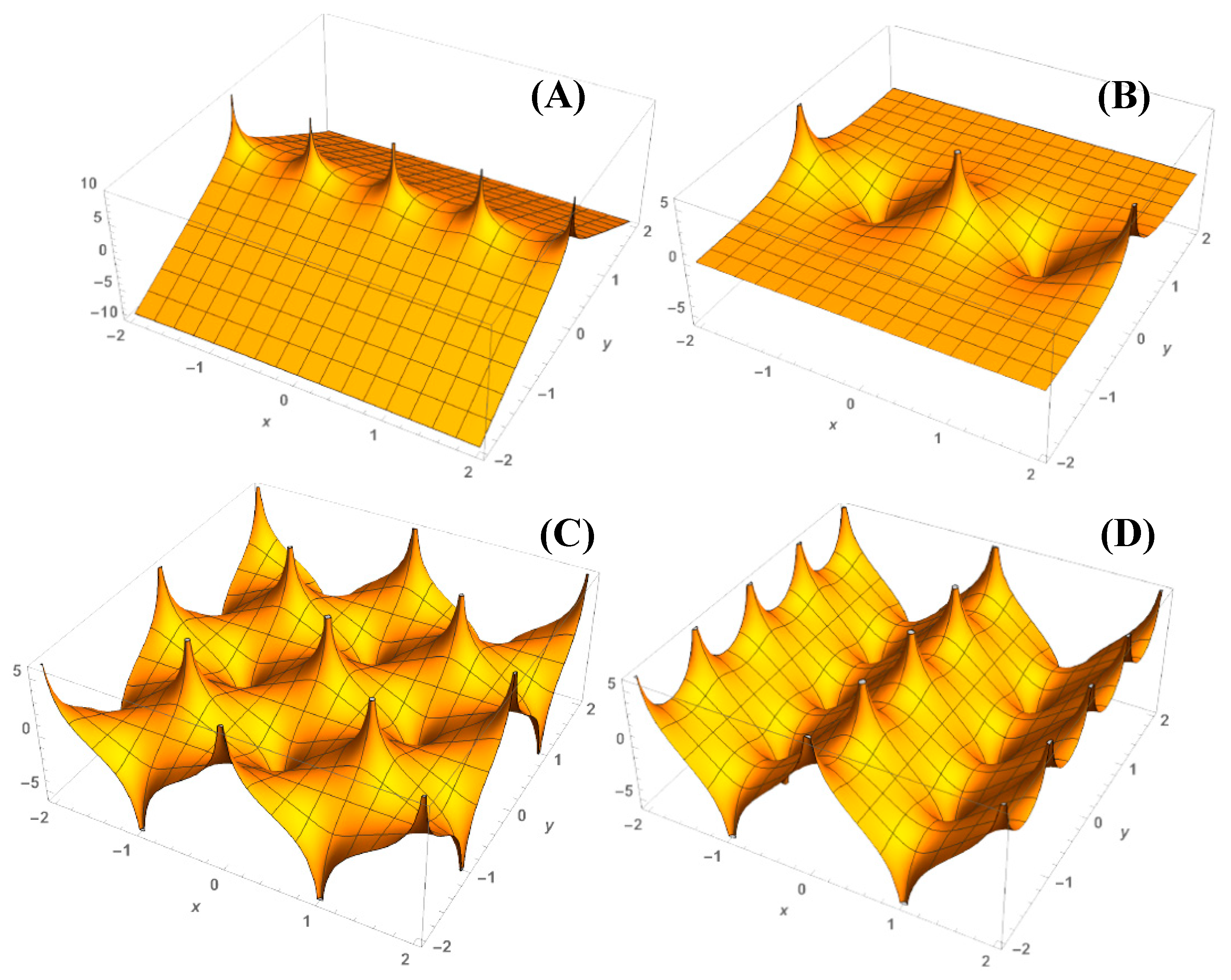
The associated line-charge arrangements are evident from Figure 1 (shown for scale $a=1$ arbitrary distance unit). The planar configuration with only positive-line charges was not considered because a large (infinite) ensemble of like charges without compensating opposites did not lead to a well-converging series.

3.2. Electric-Field Components as Sum Formulas

The following lattice series were used to calculate electric-field components in the considered cases. The electric field of a line charge is proportional to $2\lambda /r$, with $r$ being the shortest distance from the point of interest to the wire carrying the charge (compare Equation (5)).

$$\{\begin{array}{c}{E}_{A,x}\left(x,y\right)=2\lambda {\displaystyle {\displaystyle \sum }_{m=-\infty }^{\infty }}\frac{x-ma}{{\left(x-ma\right)}^2+y^2}\\ E_{A,y}\left(x,y\right)=2\lambda {\displaystyle {\displaystyle \sum }_{m=-\infty }^{\infty }}\frac{y}{{\left(x-ma\right)}^2+y^2}\end{array}$$

(7a)

$$\{\begin{array}{c}{E}_{B,x}\left(x,y\right)=2\lambda {\displaystyle {\displaystyle \sum }_{m=-\infty }^{\infty }}{\left(-1\right)}^m\frac{x-ma}{{\left(x-ma\right)}^2+y^2}\\ E_{B,y}\left(x,y\right)=2\lambda {\displaystyle {\displaystyle \sum }_{m=-\infty }^{\infty }}{\left(-1\right)}^m\frac{y}{{\left(x-ma\right)}^2+y^2}\end{array}$$

(7b)

$$\{\begin{array}{c}{E}_{C,x}\left(x,y\right)=2\lambda {\displaystyle {\displaystyle \sum }_{m,n=-\infty }^{\infty }}{\left(-1\right)}^{m+n}\frac{x-ma}{{\left(x-ma\right)}^2+{\left(y-na\right)}^2}\\ E_{C,y}\left(x,y\right)=2\lambda {\displaystyle {\displaystyle \sum }_{m,n=-\infty }^{\infty }}{\left(-1\right)}^{m+n}\frac{y-na}{{\left(x-ma\right)}^2+{\left(y-na\right)}^2}\end{array}$$

(7c)

$$\{\begin{array}{c}{E}_{D,x}\left(x,y\right)=2\lambda {\displaystyle {\displaystyle \sum }_{m,n=-\infty }^{\infty }}{\left(-1\right)}^m\frac{x-ma}{{\left(x-ma\right)}^2+{\left(y-na\right)}^2}\\ E_{D,y}\left(x,y\right)=2\lambda {\displaystyle {\displaystyle \sum }_{m,n=-\infty }^{\infty }}{\left(-1\right)}^m\frac{y-na}{{\left(x-ma\right)}^2+{(y-na)}^2}\end{array}$$

(7d)

3.3. Electric Potentials as Sum Formulas

The following lattice series were used to calculate electric potentials in the considered cases and under the convention of a zero-reference point at $\left(a/2, a/2\right)$. The formulae in Equation (7) can be obtained as the negative gradient of Equation (8).

$$U_A\left(x,y\right)=2\lambda {\displaystyle \sum }_{m=-\infty }^{\infty }\log \left[\sqrt{\frac{{\left(a/2-ma\right)}^2+{\left(a/2\right)}^2}{{\left(x-ma\right)}^2+y^2}}\right]$$

(8a)

$$U_B\left(x,y\right)=2\lambda {{\displaystyle \sum }}_{m=-\infty }^{\infty }{\left(-1\right)}^m\log \left[\sqrt{\frac{{\left(a/2-ma\right)}^2+{\left(a/2\right)}^2}{{\left(x-ma\right)}^2+y^2}}\right]$$

(8b)

$$U_C\left(x,y\right)=2\lambda {{\displaystyle \sum }}_{m,n=-\infty }^{\infty }{\left(-1\right)}^{m+n}\log \left[\sqrt{\frac{{\left(a/2-ma\right)}^2+{\left(a/2-na\right)}^2}{{\left(x-ma\right)}^2+{\left(y-na\right)}^2}}\right]$$

(8c)

$$U_D\left(x,y\right)=2\lambda {{\displaystyle \sum }}_{m,n=-\infty }^{\infty }{\left(-1\right)}^m\log \left[\sqrt{\frac{{\left(a/2-ma\right)}^2+{\left(a/2-na\right)}^2}{{\left(x-ma\right)}^2+{\left(y-na\right)}^2}}\right]$$

(8d)

3.4. Closed-Form Expressions

For the electric fields (vectors displayed in Figure 2) it holds true that:

$$E_{A,x}\left(x,y\right)-i{E}_{A,y}\left(x,y\right)=\frac{2\lambda \pi }{a}\frac{\cos \left[\pi z\right]}{\sin \left[\pi z\right]}$$

(9a)

$$E_{B,x}\left(x,y\right)-i{E}_{B,y}\left(x,y\right)=\frac{2\lambda \pi }{a}\frac{1}{\sin \left[\pi z\right]}$$

(9b)

$$E_{C,x}\left(x,y\right)-i{E}_{C,y}\left(x,y\right)=\frac{2\lambda L}{a}\frac{1}{\mathbf{sl}\left[Lz\right]}$$

(9c)

$$E_{D,x}\left(x,y\right)-i{E}_{D,y}\left(x,y\right)=\frac{\lambda L}{a}\left(\mathbf{sl}\left[Lz/2\right]\mathbf{cl}\left[Lz/2\right]+\frac{1}{\mathbf{sl}\left[Lz/2\right]\mathbf{cl}\left[Lz/2\right]}\right)$$

(9d)

where $i$ is the imaginary unit and where in each case $z=x/a+iy/a.$ To clarify: the field components are real valued, so to extract the $x$-component of the electric field in a particular case one simply needs to take the positive real part of the associated right-hand-side expression. Likewise, the $y$-component is obtained by the negative imaginary part of the right-hand-side expression.

The electric potentials are then given by:

$$U_A\left(x,y\right)=2\lambda \mathrm{Re}\left(\log \left[\frac{\cosh \left[\pi /2\right]}{\sin \left[\pi z\right]}\right]\right)$$

(10a)

$$U_B\left(x,y\right)=\lambda \mathrm{Re}\left(\log \left[\frac{1+\cos \left[\pi z\right]}{1-\cos \left[\pi z\right]}\right]\right)$$

(10b)

$$U_C\left(x,y\right)=\lambda \mathrm{Re}\left(\log \left[\frac{1+cl\left[Lz\right]}{1-cl\left[Lz\right]}\right]\right)$$

(10c)

$$U_D\left(x,y\right)=2\lambda \mathrm{Re}\left(\log \left[\frac{cl\left[Lz/2\right]}{sl\left[Lz/2\right]}\right]\right).$$

(10d)

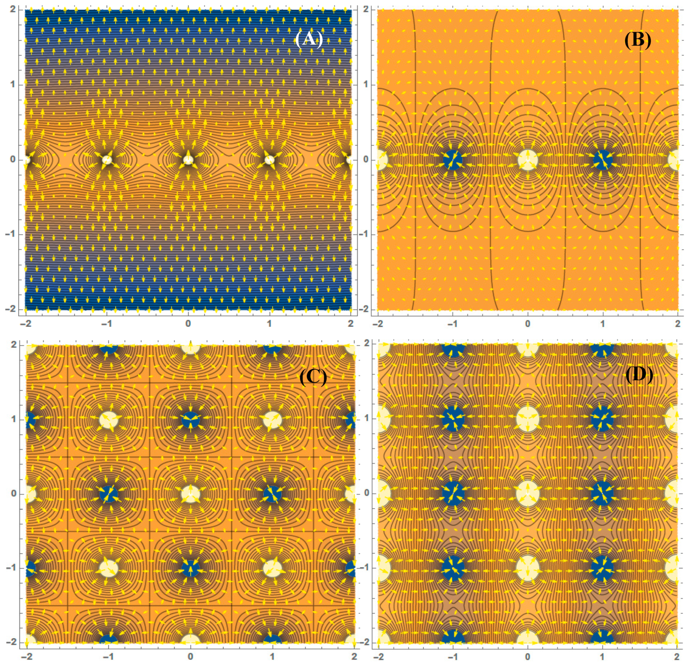
where $\mathrm{Re}$ denotes the real part and where again $z=x/a+iy/a$ in each case. Each of the electric-field Equation (9a–d) can be calculated from the corresponding potential (Equation (10a–d)) as the negative gradient. For terms containing lemniscate functions, derivatives of $\mathbf{sl}\left(\mathrm{z}\right)$ and $\mathbf{cl}\left(\mathrm{z}\right)$ can be expressed as $\mathbf{cl}\left[\mathrm{z}\right]\left(1+s{l}^2\left[\mathrm{z}\right]\right)$ and $-\mathbf{sl}\left[\mathrm{z}\right]\left(1+c{l}^2\left[\mathrm{z}\right]\right)$, respectively. All potentials quoted in Equations (8a–d) and (10a–d) satisfy the Laplace equation $\mathsf{\Delta }U=0$ in all areas of the plane without charge. The electric-field environments for the four cases are displayed in Figure 2. All field vectors crossed the equipotential lines at right angles, as expected.

4. Discussion

4.1. Comparisons to Earlier Works

The obtained solutions represent a compact way of calculating electric fields and associated potentials of infinite multiwire-grid arrays with symmetric spacing. For the trigonometric Case A, Equation (1) in [2] can be reduced via well-known trigonometric identities to our Expression (10a) using the same zero reference point for the potential. The equation presented in [2] allows also changing the spacing between line charges, so it is essentially only a matter of complex algebra to arrive at our Equation (10b) via the superposition principle. On the other hand, we have not seen in the literature accessible to us expressions using lemniscate functions as solutions to the double series. The potential associated with an analogous and more general version of Case C is treated in [17], but is reduced to a single series (see their Equation (5)), and no closed form is given. Orjubin [18] presented a solution in a line-charge configuration similar to that in Case D using a single JacobiSN function, while the potentials given here in Equation (10c,d) stay in the framework of lemniscate functions. Within [18], we found papers [19,20] written a few decades ago pioneering the use of the conformal properties of the JacobiSN elliptic function to represent fields and potentials of multigrid arrays, but we were not able to establish a direct connection of their results to those presented here. Nowadays, easy access to powerful Computer Algebra Systems (CAS systems) helps physicists (not normally deeply familiar with elliptic functions) to address these potentially difficult problems.

4.2. Duality Aspect and Corollary Findings Related to Gauss’s Constant

It appeared to us that the kind of duality between trigonometric and lemniscate functions established in this work has not yet attracted attention. To clarify what we mean by “duality” in this context, note in particular the similar formal shapes of the Case B and C solutions for the electric field components (Equation (9b,c)) as well as for the potentials (Equation (10b,c)). The superposition principle can be used to construct Case C via alternating summation of Case B arrays if properly accounting for a shift in the $y$ location of each added array of horizontal line charges. Targeting the electric field provides a simple single-series identity relating the reciprocals of the sine and the sine lemniscate functions:

$$\frac{\pi }{L}{\displaystyle \sum }_{k=-\infty }^{\infty }\frac{{\left(-1\right)}^k}{\sin \left[\pi \left(z+ik\right)\right]}=\frac{1}{\mathbf{sl}\left[Lz\right]}$$

(11)

where z is any complex number. A similar result can be obtained by swapping sin/sl for cos/cl, with the resulting identity being reminiscent of but not equivalent to Equation (12) in [13]. We found further identities of a similar kind, involving other trigonometric functions including hyperbolic functions, and uploaded these on [11]. Similar closed-form solutions can be found by applying the superposition principle to solutions for the potentials for Cases B and C.

We have thus far not mentioned that the lemniscate constant relates via $L=\pi G$ [9] to Gauss’s constant $G=0.83462$…. This, combined with Equation (11) and an observation made when viewing contours of the magnitude of the electric field in Case C, gave us confidence in the following statement: if, and only if, at least one of $2y+2x$ and $2y-2x$ is an odd integer, then

$$\left|{\displaystyle \sum }_{k=-\infty }^{\infty }\frac{{\left(-1\right)}^k}{\sin \left[\pi \left(x+i\left(y+k\right)\right)\right]}\right|=G.$$

(12)

Swapping odd integer for even integer and sin for cos in the statement gives a relationship that also holds true, meaning that, for instance, with $x=0$ and $y=0,$ we get

$${\displaystyle \sum }_{k=-\infty }^{\infty }\frac{{\left(-1\right)}^k}{\cos \left[i\pi k\right]}=G.$$

(13)

Targeting the modulus is, in this specific case, not necessary, as $\cos \left[i\pi k\right]$ is purely real for integers $k$. Replacing the numerator ${\left(-1\right)}^k$ by 1 in Equation (13), the resulting series equals $\sqrt{2}G$, (confirmed precision of >1000 digits). These latter results, given their simple appearance, may already be known. Regardless, they can be added to obtain a rather fast converging series for $G$, namely,

$$\frac{2}{1+\sqrt{2}}\left(1+2{\displaystyle \sum }_{k=1}^{\infty }\mathrm{sech}\left[2\pi k\right]\right)=G$$

(14)

where sech is the hyperbolic secant function. As an example, including only the first four terms gives an approximation of $G$ agreeing over the first 12 digits. A further observation was that Equation (6), when evaluated at $x=1/2,$ resulted in $\pi G^0$, while Equation (2) calculated to $L=\pi G^1$. We inspected the corresponding four-dimensional system ($2^2-$ dimensional system), and found that the corresponding sum equals $\pi G^2$ (verified to >100 digits). These results can be summarized as:

$$\frac{1}{\pi }{\displaystyle \sum }_{k=-\infty }^{\infty }{\left(-1\right)}^k\frac{1/2-k}{{\left(1/2-k\right)}^2}=G^0$$

(15a)

$$\frac{1}{\pi }{\displaystyle \sum }_{k,m=-\infty }^{\infty }{\left(-1\right)}^{k+m}\frac{1/2-k}{{\left(1/2-k\right)}^2+m^2}=G^1$$

(15b)

$$\frac{1}{\pi }{\displaystyle \sum }_{k,m,n,t=-\infty }^{\infty }{\left(-1\right)}^{k+m+n+t}\frac{1/2-k}{{\left(1/2-k\right)}^2+m^2+n^2+t^2}=G^2$$

(15c)

The similarly shaped sums include $2^0$, $2^1$ and $2^2$ running indices and connect to the results $G^0$, $G^1$ and $G^2$, respectively. This pattern does not seem to extend to higher powers.

4.3. Potential Applications and Extension to Asymmetric Planar Arrangements

Now the electric-field strength and potential of square geometry will be compared with the ones more familiar from circular geometry. The grid for Case C and with spacing $a=1$ is given in the Gaussian plane as tiles of unit squares. Figure 2 (lower-left panel) reveals that all straight equipotential lines, horizontally and vertically, lie exactly in the middle between positive and negative charges, where the potential is clearly zero. Conducting ground planes could be placed there without disturbing the field configuration.

The x component of the field at wall ($\mathbf{sl}\left(L/2\right)=1$) has strength

$$\left|\mathit{E}\left(1/2,0\right)\right|=\frac{2\lambda L}{\mathbf{sl}\left(L/2\right)}=2\lambda L$$

(16)

and the potential there ($\mathbf{cl}\left(L/2\right)=0$) is

$$U\left(1/2,0\right)=\lambda \mathrm{Re}\left[\log \left[\frac{1+\mathbf{cl}\left[L/2\right]}{1-\mathbf{cl}\left[L/2\right]}\right]\right]=0$$

(17)

On the other hand the radial strength of the field of a charged wire in a cylindrical tube is given as:

$$\left|E\left(r\right)\right|=\frac{2\lambda }{r}$$

(18)

and the radially symmetric potential as a function of distance is $U\left(r\right)=2\lambda \log \left[1/r\right]+C$. The boundary condition for this comparison is set to $U\left(1/2\right)=0$. From this, it follows that $C=-2\lambda \log \left[2\right]$; so finally:

$$U\left(r\right)=2\lambda \log \left[\frac{1}{2r}\right]$$

(19)

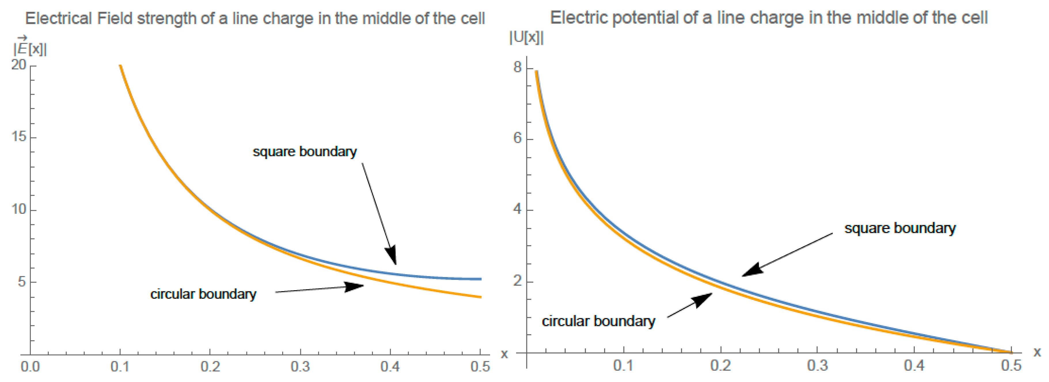
The dependence on distance of field and potential of a square and a cylindrical chamber (e.g., a Geiger counter) are contrasted in Figure 3. The electric-field comparison along the horizontal path is shown in Figure 3 left. For small $x$ away from the wall both strengths coincide well. The fields hit the wall at right angles with different strengths determined by Equations (16) and (18). There are no tangential components. The square boundary chamber has a stronger field at the wall. In Figure 3 right, we see the potentials from Equation (10c) evaluated at $y$= 0, and Equation (19) connected to the fields in the left panel. They look very similar near the wire and are zero at the boundary $x=1/2$. The surprisingly small deviation in between is due to the difference in curvature of the potentials of the two geometries imposed by the Laplace equation.

For potential applications to chambers of rectangular cross-section (like Iarocci tubes, see e.g., [17]), it is desirable to generalize our formulae to cover scenarios of different horizontal and vertical spacing between line charges. We have thus far not been able to find a closed-form solution in the framework of lemniscate functions for the generalization of Case C to arbitrary and different, horizontal and vertical line-charge spacing. Via the superposition principle, we can at least present solutions for certain simple cases of asymmetric arrangements.

Consider, for instance, the asymmetric version of Case C with horizontal spacing $a$ and vertical spacing $3a$. This arrangement may be viewed as a superposition of three horizontally shifted symmetric Case C arrangements of $3a$ spacing. The x component of the electric field is then

$$2\lambda {\displaystyle \sum }_{m,n=-\infty }^{\infty }{\left(-1\right)}^{m+n}\frac{x-ma}{{\left(x-ma\right)}^2+{\left(y-3na\right)}^2}=\frac{2\lambda L}{3a}\mathrm{Re}\left(\frac{1}{\mathbf{sl}\left[L{z}_1/3\right]}-\frac{1}{sl\left[L{z}_2/3\right]}+\frac{1}{sl\left[L{z}_3/3\right]}\right)$$

(20)

where $z_1=x/a+iy/a; z_2=x/a-1+iy/a; z_3=x/a-2+iy/a$. A minus sign in front of the second term on the right-hand side of Equation (20) appears because this particular symmetrical array carries opposite polarity compared to the other two. In asymmetric Case C, with vertical spacing being half of that of horizontal spacing, a strategy to arrive to a closed-form solution is to superpose two symmetric arrays of the Case D type, vertically shifted and of opposite polarity. The x component of the electric field is then given by

$$2\lambda {\displaystyle \sum }_{m,n=-\infty }^{\infty }{\left(-1\right)}^{m+n}\frac{x-ma}{{\left(x-ma\right)}^2+{\left(y-na/2\right)}^2}=\frac{\lambda L}{a}\mathrm{Re}\left(S\right)$$

(21a)

where

$$S=\mathbf{sl}\left[\frac{L{z}_1}{2}\right]\mathbf{cl}\left[\frac{L{z}_1}{2}\right]+\frac{1}{\mathbf{sl}\left[\frac{L{z}_1}{2}\right]\mathbf{cl}\left[\frac{L{z}_1}{2}\right]}-\mathbf{sl}\left[L{z}_2/2\right]\mathbf{cl}\left[L{z}_2/2\right]-\frac{1}{\mathbf{sl}\left[L{z}_2/2\right]\mathbf{cl}\left[L{z}_2/2\right]}$$

(21b)

with $z_1=x/a+iy/a; z_2=x/a+i\left(y/a-1/2\right)$. The $y$ component of the electric field can be obtained in both cases as the negative imaginary part. Establishing closed-form solutions for simple asymmetric versions of Case D can be done in a similar fashion, making use of superposition and solutions to symmetric versions. Inspection of Case D (see lower-right panel of Figure 2) shows that there are straight equipotential lines enclosing stripes of many charges of the same polarity, a feature encountered in certain types of chambers (cf., [18]). Their electric potential may be calculated in a similar fashion to that described above.

5. Summary and Concluding Remarks

We established closed-form expressions of electric potentials and electric fields associated with scenarios of line charges crossing a plane in various configurations. The presented cases and solutions can be combined via the superposition principle to solve for electric fields and electric potentials in other line-charge arrangements. We discussed potential physical applications of the results, and highlighted an interesting type of duality between trigonometric and lemniscate functions setting side by side, for example, Equation (9b,c), Equation (10b,c), and also the left- and right-hand parts of Equation (11). All identities presented in Section 3 are exact expressions depending on one or two variables, so that the sum and chain rules for derivatives could be applied to generate a range of corollary identities. We have listed many of these online [11].

References

- Borwein, J.M.; Glasser, M.L.; McPhedran, R.C.; Wan, J.G.; Zucker, I.J. Lattice sums then and now. In Encyclopedia of Mathematics and Its Applications; Cambridge University Press: Cambridge, UK, 2013; ISBN 978-1-107-03990-2. [Google Scholar]
- McDonald, K.T. Notes on Electrostatic Wire Grids (Published 2003). International Note. Available online: http://www.hep.princeton.edu/~mcdonald/examples/grids.pdf (accessed on 1 June 2020).
- Weertman, J. Dislocation Based Fracture Mechanics; World Scientific Publishing Company: Singapore, 1996; ISBN 978-9-813-10497-6. [Google Scholar]
- Gradshteyn, I.S.; Ryzhik, I.M. Table of Integrals, Series and Products, 7th ed.; Academic Press, Elsevier Inc.: Cambridge, MA, USA, 2007; ISBN 978-0-12-373637-6. [Google Scholar]
- Hansen, E.R.A. A Table of Series and Products; Prentice-Hall: Upper Saddle River, NJ, USA, 1975; ISBN 978-0-13-881935-5. [Google Scholar]
- Prudnikov, A.P.; Brychkov, Y.A.; Marichev, O.I. Integrals and Series; Gordon and Breach Science Publishers: New York, NY, USA, 1986–1992; Volumes 1–3. [Google Scholar]
- Markushevich, A.I. The Remarkable Sine Functions; American Elsevier Publishing Company: Amsterdam, The Netherlands, 1966. [Google Scholar]
- Eberhard, Z. Oxford Users’ Guide to Mathematics; Oxford University Press: Oxford, UK, 2004; ISBN 978-0-198-50763-5. [Google Scholar]
- Young, R.M. Excursions in Calculus: An Interplay of the Continuous and the Discrete; Cambridge University Press: Cambridge, UK, 1992; Volume 13, ISBN 978-0-883-85317-7. [Google Scholar]
- Lemniscate Functions. E.D. Solomontsev (Originator), Encyclopedia of Mathematics. Available online: http://encyclopediaofmath.org/index.php?title=Lemniscate_functions&oldid=17903 (accessed on 27 May 2020).
- A Collection of Infinite Products and Series (Andreas Dieckmann). Available online: http://www-elsa.physik.uni-bonn.de/~dieckman/InfProd/InfProd.html (accessed on 16 May 2020).
- The Online Encyclopedia of Integer Sequences (N. J. A. Sloane). Available online: https://oeis.org (accessed on 16 May 2020).
- Boyd, J.P. New series for the cosine lemniscate function and the polynomialization of the lemniscate integral. J. Comput. Appl. Math. 2011, 235, 1941–1955. [Google Scholar] [CrossRef] [Green Version]
- Wolfram Research, Inc. Mathematica, Version 12.1; Wolfram Research, Inc.: Champaign, IL, USA, 2020.
- Purcell, E.M. Electricity and Magnetism (Berkeley Physics Course, Vol.2); McGraw-Hill: New York, NY, USA, 1966; ISBN 978-0-070-04908-6. [Google Scholar]
- Table of Integrals (Andreas Dieckmann). Available online: http://www-elsa.physik.uni-bonn.de/~dieckman (accessed on 29 May 2020).
- Lu, C.; McDonald, K. The Electric Potential of Particle Detectors with Rectangular Cross-Section (Published 2002). Available online: http://puhep1.princeton.edu/~mcdonald/examples/iarocci.pdf (accessed on 1 June 2020).
- Orjubin, G. Closed-form expressions of the electrostatic potential close to a grid placed between two plates. J. Electrost. 2017, 87, 195–202. [Google Scholar] [CrossRef]
- Tomitani, T. Analysis of potential distribution in a gaseous counter of rectangular cross-section. Nucl. Instr. Methods 1972, 100, 179–191. [Google Scholar] [CrossRef]
- Cooperman, P. A theory for space-charge-limited currents with application to electrical precipitation. AIEE Trans. 1960, 79, 47–50. [Google Scholar] [CrossRef]
Figure 1.
Sections of size of electric potentials corresponding to Cases (A) (upper left), (B) (upper right), (C) (lower left) and (D) (lower right). Reference points set such that and were set to 1.
Figure 2.
Equipotential lines and electric-field vectors of potential section shown in Figure 1 for Cases (A), (B), (C) and (D) as indicated. Blue/yellow areas are below/above the chosen reference point of each potential. Space between charges shown in ochre carried potential values near zero. All potentials, lines, and vectors drawn using closed expressions from Equations (8)–(10), setting a and to 1. ContourPlots with overlayed VectorPlots are shown using automatic vector scaling.
Figure 3.
(left) Field strengths and (right) electric potentials of (blue line) square tube and (orange line) Geiger counter, shown decreasing from the wire edge to the grounded wall.
© 2020 by the authors. Licensee MDPI, Basel, Switzerland. This article is an open access article distributed under the terms and conditions of the Creative Commons Attribution (CC BY) license (http://creativecommons.org/licenses/by/4.0/).
Share and Cite
MDPI and ACS Style
Vigren, E.; Dieckmann, A. Simple Solutions of Lattice Sums for Electric Fields Due to Infinitely Many Parallel Line Charges. Symmetry 2020, 12, 1040. https://0-doi-org.brum.beds.ac.uk/10.3390/sym12061040
AMA Style
Vigren E, Dieckmann A. Simple Solutions of Lattice Sums for Electric Fields Due to Infinitely Many Parallel Line Charges. Symmetry. 2020; 12(6):1040. https://0-doi-org.brum.beds.ac.uk/10.3390/sym12061040
Chicago/Turabian StyleVigren, Erik, and Andreas Dieckmann. 2020. "Simple Solutions of Lattice Sums for Electric Fields Due to Infinitely Many Parallel Line Charges" Symmetry 12, no. 6: 1040. https://0-doi-org.brum.beds.ac.uk/10.3390/sym12061040
Note that from the first issue of 2016, this journal uses article numbers instead of page numbers. See further details here.