A Robust q-Rung Orthopair Fuzzy Einstein Prioritized Aggregation Operators with Application towards MCGDM

Abstract

A q-rung orthopair fuzzy set (q-ROFS) provides a significant mechanism for managing symmetrical aspects in real life circumstances. The renowned distinguishing feature of q-ROFS is that the sum of the qth powers to each membership degree (MD) and non-membership degree (NMD) is less than or equal 1, and therefore the comprehensive uncertain space for q-ROF information is broader. Numerous researchers have suggested several aggregation operators based on q-ROFSs. In order to discuss prioritized relationship in the criterion and a smooth approximation of q-ROF information, we introduced q-rung orthopair fuzzy Einstein prioritized weighted averaging (q-ROFEPWA) operator and q-rung orthopair fuzzy Einstein prioritized weighted geometric (q-ROFEPWG) operator. Additionally, we presented a multi-criteria group decision making (MCGDM) technique based on q-rung orthopair fuzzy Einstein prioritized aggregation operators. These operators can evaluate the possible symmetric roles of the criterion that express the real phenomena of the problem. In order to investigate characteristic of suggested operators regarding the symmetry of attributes and their symmetrical roles under q-ROF information, we presented an application of Einstein prioritized aggregation operators. Finally, by comparing it with some other established representative MCGDM models, an illustrative example is provided to check the feasibility, efficiency and supremacy of the proposed technique.

1. Introduction

Issues concerning unstable situations typically arise in decision-making, but they are demanding because of the complex and difficult situation of modeling and manipulation that emerges with such uncertainties. In an attempt to solve complex real-world problems, methods widely used in classical mathematics are often not useful due to the different kinds of complexity and lack of clarity in these important issues. To deal with uncertainties and vagueness. Zadeh initiated fuzzy set theory [1], Atanassov [2] introduced intuitionistic fuzzy sets (IFSs) and Yager [3,4,5] presented the notion of Pythagorean fuzzy sets. Zhang [6] introduced bipolar fuzzy sets and relations.

Several researchers have analyzed implementations of fuzzy sets; Ali et al. [7], Ali [8], Chen et al. [9], Chi and Lui [10], Çağman et al. [11], Eraslan and Karaaslan [12], Feng et al. [13,14,15,16] presented some work about soft sets combined with fuzzy sets and rough sets, Garg and Arora [17,18,19] introduced some aggregation operators (AOs) related to IFS, soft set and application related to MCDM, Kumar and Garg [20], Karaaslan [21], Liu et al. [22], Naeem et al. [23,24,25] introduced PFS with m-polar, Peng et al. [26,27,28,29] gave some results related to PFS, Riaz and Hashmi [30,31] presented a novel concept of linear diophantine fuzzy set, Riaz et al. [32], Riaz and Tehrim [33,34], Shabir and Naz [35], Wang et al. [36], Xu [37], Xu and Cai [38], Xu [39], Xu developed a number of AOs, based on IFSs [37], Ye [40,41], Zhang and Xu [42], Zhan et al. [43,44] presented some aggregation techniques and Zhang et al. [45,46,47] presented work of rough set, Riaz et al. [48,49] presented some AOs of q-ROFSs. Sharma et al. [50] and Sinani et al. [51] presented some work related to rough set theory.

Yager initiated the idea of q-ROFS as an extension of PFS [52], in which the sum of membership degree (MD) ${\check{\mathfrak{p}}}_A(\zeta )$ and non-membership degree (NMD) ${\overline{⨿}}_A(\zeta )$ satisfy the condition $0\le {\left({\check{\mathfrak{P}}}_A(\zeta )\right)}^q+{\left({\overline{⨿}}_A(\zeta )\right)}^q\le 1,(q\ge 1)$. The degree of indeterminacy (ID) is given by ${\pi }_A(\zeta )=\sqrt[q]{({\check{\mathfrak{P}}}_A^q(\zeta )+{\overline{⨿}}_A^q(\zeta )-{\check{\mathfrak{P}}}_A^q(\zeta ){\overline{⨿}}_A^q(\zeta ))}$. There is no condition on q other than $q\ge 1$. Although q is real number, but if q is integral value, it is also very easy to predict the area from which MD and NMD are selected. We can easily check that $99\%$ area is covered when we put $q=10$ of unit square $[0,1]\times [0,1]$.

Aggregation operators (AOs) are effective tools, particularly in the multi-criteria group decision making (MCGDM) analysis, to merge all input arguments into one completely integrated value. Since Yager introduced the classic OWA operator, different varieties of AOs were studied and applied to various decision-making issues [53]. Yager developed many weighted average, weighted geometric and ordered weighted AOs based on PFSs. Grag [54] and Rahmana et al. [55] introduced some Einstein AOs on PFS. Khan et al. [56] initiated the concept of prioritized AOs and also Einstein prioritized [57] on PFS. However, there has indeed been very few research on AOs in the context of q-ROF. In the available literature, relying on the proposed operation of q-rung orthopair fuzzy numbers (q-ROFNs). Liu and Wang [58] have established several more basic q-ROF AOs. Liu and Liu [59] drawn-out the Bonferroni mean AOs to q-ROF environment. Zhao [60] introduced some hammy mean AOs to aggregate the q-ROFNs. The AOs suggested above for q-ROFNs claiming that the parameters is of the same level of severity. Even so, this assumption may not always be usable in several practical issues. In this article we are specifically exploring the MCGDM issue where a priority relationship occurs over the parameters. The criteria are at different priority stages. Consider the issue in which we pick a new car on the basis of safeness, cost, presence and performance measures. We are not willing to sacrifice safeness for cost-effectiveness. First, we consider the safety requirements, then we consider the cost and finally, we consider appearance and performance. There is a prioritization relationship over the criteria in this situation. Protection has a greater priority than costs. Cost has a higher priority than appearance and performance.

About the question: why have we been developing all this research? If we consider existing aggregation operators, they have not provided us with a smooth approximation. There are several types of groups of t-norms and t-norms that can be chosen to construct intersections and unions. Einstein sums and Einstein products are good alternatives to algebraic sums and algebraic products because they provide a very smooth approximation. If we have a case in which we have a prioritized relationship in criteria and we also have a smooth approximation, we use the proposed aggregation operators.

In the rest of this paper: Section 2 consists of key characteristics for fuzzy sets, IFSs and q-ROFSs. Section 3 introduces some newly aggregation operators (AOs) based on q-ROFSs and their characteristics. Section 4 provides the proposed methodology to deal MCGDM problems. In Section 5 we give a concrete example of the effectiveness and viability of the suggested approach and also present comparison analysis with other techniques. Finally, whole paper is summarized in Section 6.

2. Preliminaries

In 1986, Atanassov developed the concept of IFS as a generalization of Zadeh’s fuzzy set, and it should be noted that IFS is an important way of dealing with vagueness and lack of consensus.

Definition 1.

Let$\breve{\Psi }=({\zeta }_1,{\zeta }_2,\dots {\zeta }_n)$be a finite set, then an IFS, $\breve{J}$ in$\breve{\Psi }$can described as follows:

$$\breve{J}=\{<\zeta ,{\check{\mathfrak{P}}}_{\breve{J}}(\zeta ),{\overline{⨿}}_{\breve{J}}(\zeta )>:\zeta \in \breve{\Psi }\}$$

(1)

where ${\check{\mathfrak{P}}}_{\breve{J}}(\zeta )$ and${\overline{⨿}}_{\breve{J}}(\zeta )$are mappings from$\breve{\Psi }$to $[0,1]$, ${\check{\mathfrak{P}}}_{\breve{J}}(\zeta )$ is called MD and${\overline{⨿}}_{\breve{J}}(\zeta )$is called NMD with conditions, $0\le {\check{\mathfrak{P}}}_{\breve{J}}(\zeta )\le 1$,$0\le {\overline{⨿}}_{\breve{J}}(\zeta )\le 1$and$0\le {\check{\mathfrak{P}}}_{\breve{J}}(\zeta )+{\overline{⨿}}_{\breve{J}}(\zeta )\le 1$,$\forall \zeta \in \breve{\Psi }$. ${\pi }_{\breve{J}}(\zeta )=1-({\check{\mathfrak{P}}}_{\breve{J}}(\zeta )+{\overline{⨿}}_{\breve{J}}(\zeta ))$is called ID of $\breve{J}$ in $\breve{\Psi }$. In addition,$0\le {\pi }_{\breve{J}}(\zeta )\le 1$$\forall \zeta \in \breve{\Psi }$.

Since IFS meets the limitations that the sum of its MD and NMD would be less than or equal to 1. Fortunately, the DM can handle the scenario in which the sum of MD and NMD is higher than unity in complex decision-making problem. Therefore, Yager introduced the concept of PFS to resolve this situation, which satisfies the constraints that the square sum of its MD and NMD should be less than or equal to 1.

Definition 2.

Let $\breve{\Psi }=({\zeta }_1,{\zeta }_2,\dots {\zeta }_n)$ be a finite set, then an PFS, $\breve{P}$ in $\breve{\Psi }$ can described as follows:

$$\breve{P}=\{<\zeta ,{\check{\mathfrak{P}}}_{\breve{P}}(\zeta ),{\overline{⨿}}_{\breve{P}}(\zeta )>:\zeta \in \breve{\Psi }\}$$

(2)

where ${\check{\mathfrak{P}}}_{\breve{P}}(\zeta )$ and ${\overline{⨿}}_{\breve{P}}(\zeta )$ are mappings from $\breve{\Psi }$ to $[0,1]$, ${\check{\mathfrak{P}}}_{\breve{P}}(\zeta )$ is called MD and ${\overline{⨿}}_{\breve{P}}(\zeta )$ is called NMD with conditions, $0\le {\check{\mathfrak{P}}}_{\breve{P}}(\zeta )\le 1$, $0\le {\overline{⨿}}_{\breve{P}}(\zeta )\le 1$ and $0\le {\check{\mathfrak{P}}}_{\breve{P}}^2(\zeta )+{\overline{⨿}}_{\breve{P}}^2(\zeta )\le 1$, $\forall \zeta \in \breve{\Psi }$. ${\pi }_{\breve{P}}(\zeta )=\sqrt{1-({\check{\mathfrak{P}}}_{\breve{P}}^2(\zeta )+{\overline{⨿}}_{\breve{P}}^2(\zeta ))}$ is called ID of $\breve{P}$ in $\breve{\Psi }$. In addition, $0\le {\pi }_{\breve{P}}(\zeta )\le 1$$\forall \zeta \in \breve{\Psi }$.

There is still a problem with DM’s question as to whether the square sum of MD and NMD is greater than one. To solve this problem, again Yager initiated the idea of q-ROFS in which the sum of $q^{th}$ power of MD and NMD is less or equal to 1.

Definition 3.

Let $\breve{\Psi }=({\zeta }_1,{\zeta }_2,\dots {\zeta }_n)$ be a finite universal set, then a q-ROFS, $\breve{H}$ in $\breve{\Psi }$ can described as follows:

$$\breve{H}=\{<\zeta ,{\check{\mathfrak{P}}}_{\breve{H}}(\zeta ),{\overline{⨿}}_{\breve{H}}(\zeta )>:\zeta \in \breve{\Psi }\}$$

(3)

where ${\check{\mathfrak{P}}}_{\breve{H}}(\zeta )$ and ${\overline{⨿}}_{\breve{H}}(\zeta )$ are mappings from $\breve{\Psi }$ to $[0,1]$, ${\check{\mathfrak{P}}}_{\breve{H}}(\zeta )$ is called MD and ${\overline{⨿}}_{\breve{H}}(\zeta )$ is called NMD with conditions, $0\le {\check{\mathfrak{P}}}_{\breve{H}}(\zeta )\le 1$, $0\le {\overline{⨿}}_{\breve{H}}(\zeta )\le 1$ and $0\le {\check{\mathfrak{P}}}_{\breve{H}}^q(\zeta )+{\overline{⨿}}_{\breve{H}}^q(\zeta )\le 1$$q\ge 1$, $\forall \zeta \in \breve{\Psi }$. ${\pi }_{\breve{H}}(\zeta )=\sqrt[q]{1-({\check{\mathfrak{P}}}_{\breve{H}}^q(\zeta )+{\overline{⨿}}_{\breve{H}}^q(\zeta ))}$ is called ID of $\breve{H}$ in $\breve{\Psi }$. In addition, $0\le {\pi }_{\breve{H}}(\zeta )\le 1$$\forall \zeta \in \breve{\Psi }$. For each $\zeta \in \breve{\Psi }$, a basic element of the form $\langle {\check{\mathfrak{P}}}_{\breve{H}}(\zeta ),{\overline{⨿}}_{\breve{H}}(\zeta )\rangle$ in a q-ROFS, denoted by $\ddot{\mathfrak{S}}$, is called q-ROFN. It could be given as $\ddot{\mathfrak{S}}=\langle {\check{\mathfrak{P}}}_{\breve{H}},{\overline{⨿}}_{\breve{H}}\rangle$.

Liu further suggested to aggregate the q-ROFN with the following operational rules.

Definition 4

([58]). Let ${\ddot{\mathfrak{S}}}_1=\langle {\check{\mathfrak{P}}}_1,{\overline{⨿}}_1\rangle$ and ${\ddot{\mathfrak{S}}}_2=\langle {\check{\mathfrak{P}}}_2,{\overline{⨿}}_2\rangle$ be q-ROFNs. Then

$$\overline{{\ddot{\mathfrak{S}}}_1}=\langle {\overline{⨿}}_1,{\check{\mathfrak{P}}}_1\rangle$$

(4)

$${\ddot{\mathfrak{S}}}_1\vee {\ddot{\mathfrak{S}}}_2=\langle max\{{\check{\mathfrak{P}}}_1,{\overline{⨿}}_1\},min\{{\check{\mathfrak{P}}}_2,{\overline{⨿}}_2\}\rangle$$

(5)

$${\ddot{\mathfrak{S}}}_1\wedge {\ddot{\mathfrak{S}}}_2=\langle min\{{\check{\mathfrak{P}}}_1,{\overline{⨿}}_1\},max\{{\check{\mathfrak{P}}}_2,{\overline{⨿}}_2\}\rangle$$

(6)

$${\ddot{\mathfrak{S}}}_1\oplus {\ddot{\mathfrak{S}}}_2=\langle \sqrt[q]{({\check{\mathfrak{P}}}_1^q+{\check{\mathfrak{P}}}_2^q-{\check{\mathfrak{P}}}_1^q{\check{\mathfrak{P}}}_2^q)},{\overline{⨿}}_1{\overline{⨿}}_2\rangle$$

(7)

$${\ddot{\mathfrak{S}}}_1\otimes {\ddot{\mathfrak{S}}}_2=\langle {\check{\mathfrak{P}}}_1{\check{\mathfrak{P}}}_2,\sqrt[q]{({\overline{⨿}}_1^q+{\overline{⨿}}_2^q-{\overline{⨿}}_1^q{\overline{⨿}}_2^q)}\rangle$$

(8)

$$\sigma {\ddot{\mathfrak{S}}}_1=\langle \sqrt[q]{1-{(1-{\check{\mathfrak{P}}}_1^q)}^{\sigma }},{\overline{⨿}}_1^{\sigma }\rangle$$

(9)

$${\ddot{\mathfrak{S}}}_1^{\sigma }=\langle {\check{\mathfrak{P}}}_1^{\sigma },\sqrt[q]{1-{(1-{\overline{⨿}}_1^q)}^{\sigma }}\rangle$$

(10)

Definition 5.

Suppose $\tilde{\Re }=\langle \check{\mathfrak{P}},\overline{⨿}\rangle$ is a q-ROFN, then a score function $\mathfrak{E}$ of $\tilde{\Re }$ is defined as

$$\mathfrak{E}(\tilde{\Re })={\check{\mathfrak{P}}}^q-{\overline{⨿}}^q$$

$\mathfrak{E}(\tilde{\Re })\in [-1,1]$. The score of a q-ROFN defines its ranking i.e., high score defines high preference of q-ROFN. However, score function is not useful in many cases of q-ROFN. For example, let us consider ${\ddot{\mathfrak{S}}}_1=\langle 0.6138,0.2534\rangle$ and ${\ddot{\mathfrak{S}}}_2=\langle 0.7147,0.4453\rangle$ are two q-ROFN, if we take value of q is 2. Then $\mathfrak{E}({\ddot{\mathfrak{S}}}_1)=0.3125=\mathfrak{E}({\ddot{\mathfrak{S}}}_2)$ i.e., score function of ${\ddot{\mathfrak{S}}}_1$ and ${\ddot{\mathfrak{S}}}_2$ are same. Therefore, to compare the q-ROFNs, it is not necessary to rely on the score function. We add a further method, the accuracy function, to solve this issue.

Definition 6.

Suppose $\tilde{\Re }=\langle \check{\mathfrak{P}},\overline{⨿}\rangle$ is a q-ROFN, then an accuracy function $\mathfrak{R}$ of $\tilde{\Re }$ is defined as

$$\mathfrak{R}(\tilde{\Re })={\check{\mathfrak{P}}}^q+{\overline{⨿}}^q$$

$\mathfrak{R}(\tilde{\Re })\in [0,1]$. The high value of accuracy degree $\mathfrak{R}(\tilde{\Re })$ defines high preference of $\tilde{\Re }$.

Again consider ${\ddot{\mathfrak{S}}}_1=\langle 0.6138,0.2534\rangle$ and ${\ddot{\mathfrak{S}}}_2=\langle 0.7147,0.4453\rangle$ two q-ROFNs. Then their accuracy functions are $\mathfrak{R}({\ddot{\mathfrak{S}}}_1)=0.4410$ and $\mathfrak{R}({\ddot{\mathfrak{S}}}_2)=0.4410$, so by accuracy function we have ${\ddot{\mathfrak{S}}}_1<{\ddot{\mathfrak{S}}}_2$.

Definition 7.

Let $\yen =\langle {\check{\mathfrak{P}}}_{\yen },{\overline{⨿}}_{\yen }\rangle$ and $\mathfrak{M}=\langle {\check{\mathfrak{P}}}_{\mathfrak{M}},{\overline{⨿}}_{\mathfrak{M}}\rangle$ are q-ROFNs, and $\mathfrak{E}(\yen ),\mathfrak{E}(\mathfrak{M})$ are the score function of ¥ and $\mathfrak{M}$, and $\mathfrak{R}(\yen ),\mathfrak{R}(\mathfrak{M})$ are the accuracy function of ¥ and $\mathfrak{M}$, then

 (1) 

If $\mathfrak{E}(\yen )>\mathfrak{E}(\mathfrak{M})$, then $\yen >\mathfrak{M}$

 (2) 

If $\mathfrak{E}(\yen )=\mathfrak{E}(\mathfrak{M})$, then

• if $\mathfrak{R}(\yen )>\mathfrak{R}(\mathfrak{M})$ then $\yen >\mathfrak{M}$,
• if $\mathfrak{R}(\yen )=\mathfrak{R}(\mathfrak{M})$, then $\yen =\mathfrak{M}$.

It should always be noticed that the value of score function is between –1 and 1. We introduce another score function, to support the following research, $\breve{\Xi }(\Re )=\frac{1+{\check{\mathfrak{P}}}_{\Re }^q-{\overline{⨿}}_{\Re }^q}{2}$. We can see that $0\le \breve{\Xi }(\Re )\le 1$. This new score function satisfies all properties of score function defined by Yager [52].

2.1. The Study’s Motivation and Intense Focus

In this subsection, we put a light on the scope, motivation and novelty of proposed work.

• This article covers two main issues: the theoretical model of the problem and the application of decision-making.
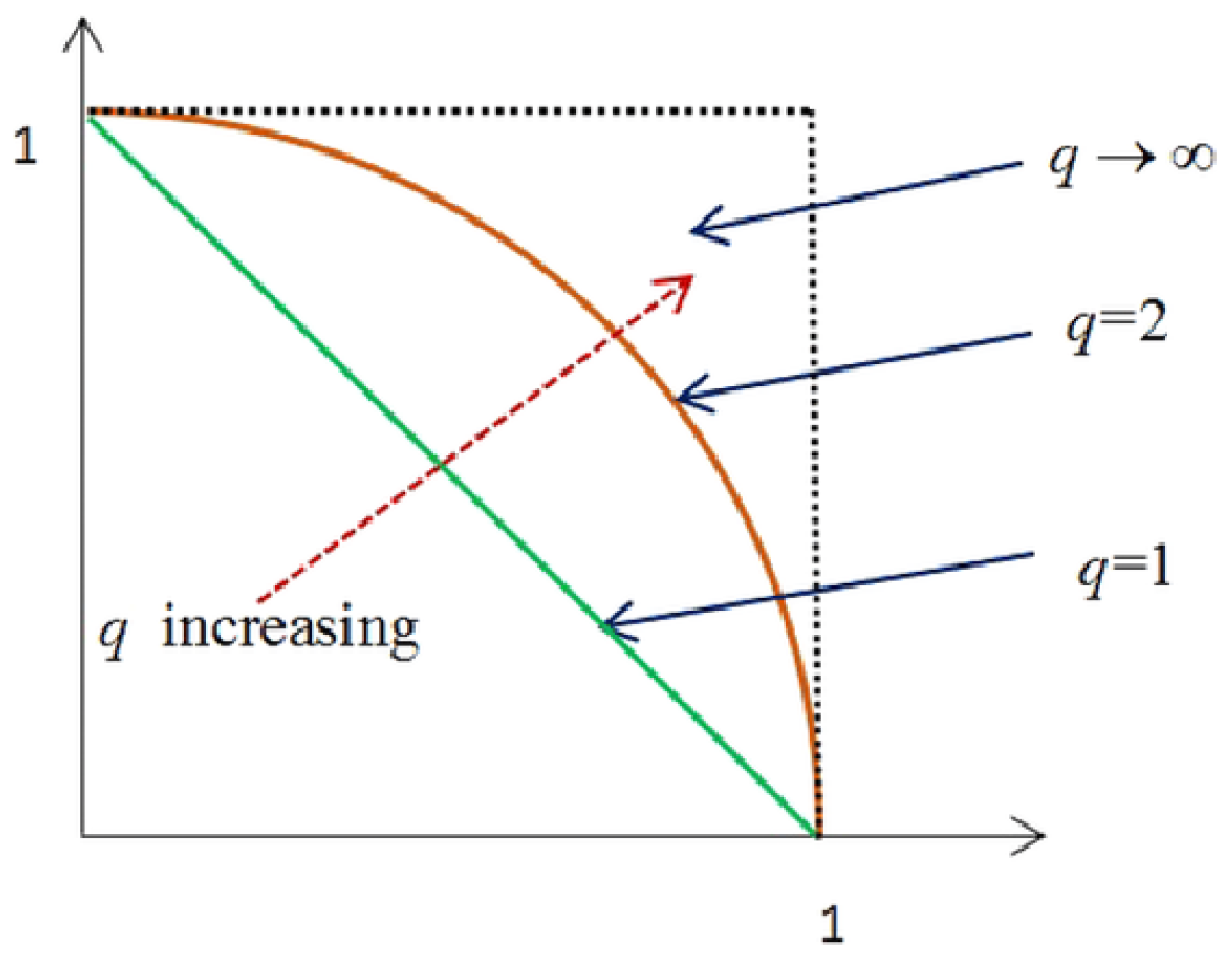
• The proposed models of aggregated operators are credible, valid, versatile and better than the rest to others because they will be based on the generalized q-ROFN structure. If the suggested operators are used in the context of IFNs or PFNs, the results will be ambiguous leading to the decrease of information in the inputs. This loss is due to restrictions on membership and non-membership of IFNs and PFNs. (see Figure 1). The IFNs and PFNs become special cases of q-ROFNs when $q=1$ and $q=2$ respectively.
• The main objective is to establish strong relationships with the multi-criteria decision-making issues between the proposed operators. The application shall communicate the effectiveness, interpretation and motivation of the proposed aggregated operators.
• This research fills the research gap and provides us a wide domain for the input data selection in medical, business, artificial intelligence, agriculture, and engineering. We can tackle those problems which contain ambiguity and uncertainty due to its limitations. The results obtained by using proposed operators and q-ROFNs will be superior and profitable in decision-making techniques.

For q-ROFNs, Riaz et al. [48] introduced the Einstein operation and studied the desirable properties of these operations. with the help of these operation they developed q-ROFEWA and q-ROFEWG operators.

Definition 8

([48]). Let ${\ddot{\mathfrak{S}}}_1=\langle {\check{\mathfrak{P}}}_1,{\overline{⨿}}_1\rangle$ and ${\ddot{\mathfrak{S}}}_2=\langle {\check{\mathfrak{P}}}_2,{\overline{⨿}}_2\rangle$ be q-ROFNs, $\mathfrak{w}>0$ be real number, then

$$\overline{{\ddot{\mathfrak{S}}}_1}=\langle {\overline{⨿}}_1,{\check{\mathfrak{P}}}_1\rangle$$

(11)

$${\ddot{\mathfrak{S}}}_1{\vee }_{ϵ}{\ddot{\mathfrak{S}}}_2=\langle \mathit{max}\{{\check{\mathfrak{P}}}_1,{\check{\mathfrak{P}}}_2\},\mathit{min}\{{\overline{⨿}}_1,{\overline{⨿}}_2\}\rangle$$

(12)

$${\ddot{\mathfrak{S}}}_1{\wedge }_{ϵ}{\ddot{\mathfrak{S}}}_2=\langle \mathit{min}\{{\check{\mathfrak{P}}}_1,{\check{\mathfrak{P}}}_2\},\mathit{max}\{{\overline{⨿}}_1,{\overline{⨿}}_2\}\rangle$$

(13)

$${\ddot{\mathfrak{S}}}_1{\otimes }_{ϵ}{\ddot{\mathfrak{S}}}_2=〈\frac{{\check{\mathfrak{P}}}_{1·ϵ}{\check{\mathfrak{P}}}_2}{\sqrt[q]{1+(1-{\check{\mathfrak{P}}}_1^q{)}_{·ϵ}(1-{\check{\mathfrak{P}}}_2^q)}},\sqrt[q]{\frac{{\overline{⨿}}_1^q+{\overline{⨿}}_2^q}{1+{\overline{⨿}}_{1·ϵ}^q{\overline{⨿}}_2^q}}〉$$

(14)

$${\ddot{\mathfrak{S}}}_1{\oplus }_{ϵ}{\ddot{\mathfrak{S}}}_2=〈\sqrt[q]{\frac{{\check{\mathfrak{P}}}_1^q+{\overline{⨿}}_2^q}{1+{{\check{\mathfrak{P}}}_1^q}_{·ϵ}{\check{\mathfrak{P}}}_2^q}},\frac{{\overline{⨿}}_{1·ϵ}{\overline{⨿}}_2}{\sqrt[q]{1+(1-{\overline{⨿}}_1^q{)}_{·ϵ}(1-{\overline{⨿}}_2^q)}}〉$$

(15)

$${\mathfrak{w}}_{·ϵ}{\ddot{\mathfrak{S}}}_1=〈\sqrt[q]{\frac{{(1+{({\check{\mathfrak{P}}}_1)}^q)}^{\mathfrak{w}}-{(1-{({\check{\mathfrak{P}}}_1)}^q)}^{\mathfrak{w}}}{{(1+{({\check{\mathfrak{P}}}_1)}^q)}^{\mathfrak{w}}+{(1-{({\check{\mathfrak{P}}}_1)}^q)}^{\mathfrak{w}}}},\frac{\sqrt[q]{2}{({\overline{⨿}}_1)}^{\mathfrak{w}}}{\sqrt[q]{{(2-{({\check{\mathfrak{P}}}_1)}^q)}^{\mathfrak{w}}+{({({\overline{⨿}}_1)}^q)}^{\mathfrak{w}}}}〉$$

(16)

$${\ddot{\mathfrak{S}}}_1^{\mathfrak{w}}=〈\frac{\sqrt[q]{2}{({\check{\mathfrak{P}}}_1)}^{\mathfrak{w}}}{\sqrt[q]{{(2-{({\check{\mathfrak{P}}}_1)}^q)}^{\mathfrak{w}}+{({({\check{\mathfrak{P}}}_1)}^q)}^{\mathfrak{w}}}},\sqrt[q]{\frac{{(1+{({\overline{⨿}}_1)}^q)}^{\mathfrak{w}}-{(1-{({\overline{⨿}}_1)}^q)}^{\mathfrak{w}}}{{(1+{({\overline{⨿}}_1)}^q)}^{\mathfrak{w}}+{(1-{({\overline{⨿}}_1)}^q)}^{\mathfrak{w}}}}〉$$

(17)

Theorem 1

([48]). Let ${\ddot{\mathfrak{S}}}_1$ and ${\ddot{\mathfrak{S}}}_2$ be q-ROFNs and $\mathfrak{w},{\mathfrak{w}}_1,{\mathfrak{w}}_2\ge 0$ be any real number, then

 (i) 

${\ddot{\mathfrak{S}}}_2{\otimes }_{ϵ}{\ddot{\mathfrak{S}}}_1={\ddot{\mathfrak{S}}}_1{\otimes }_{ϵ}{\ddot{\mathfrak{S}}}_2$

 (ii) 

${\ddot{\mathfrak{S}}}_2{\oplus }_{ϵ}{\ddot{\mathfrak{S}}}_1={\ddot{\mathfrak{S}}}_1{\oplus }_{ϵ}{\ddot{\mathfrak{S}}}_2$

 (iii) 

${({\ddot{\mathfrak{S}}}_2{\otimes }_{ϵ}{\ddot{\mathfrak{S}}}_1)}^{\mathfrak{w}}={\ddot{\mathfrak{S}}}_2^{\mathfrak{w}}{\otimes }_{ϵ}{\ddot{\mathfrak{S}}}_1^{\mathfrak{w}}$

 (iv) 

${\mathfrak{w}}_{·ϵ}({\ddot{\mathfrak{S}}}_1{\oplus }_{ϵ}{\ddot{\mathfrak{S}}}_2)={\mathfrak{w}}_{·ϵ}{\ddot{\mathfrak{S}}}_1{\oplus }_{ϵ}{\mathfrak{w}}_{·ϵ}{\ddot{\mathfrak{S}}}_2$

 (v) 

${\ddot{\mathfrak{S}}}_1^{{\mathfrak{w}}_1}{\otimes }_{ϵ}{\ddot{\mathfrak{S}}}_1^{{\mathfrak{w}}_2}={\ddot{\mathfrak{S}}}_1^{{\mathfrak{w}}_1+{\mathfrak{w}}_2}$

 (vi) 

${\mathfrak{w}}_{1·ϵ}({\mathfrak{w}}_{2·ϵ}{\ddot{\mathfrak{S}}}_1)=({\mathfrak{w}}_{1·ϵ}{\mathfrak{w}}_2{)}_{·ϵ}{\ddot{\mathfrak{S}}}_1$

 (vii) 

${({\ddot{\mathfrak{S}}}_1^{{\mathfrak{w}}_1})}^{{\mathfrak{w}}_2}={({\ddot{\mathfrak{S}}}_1)}^{{\mathfrak{w}}_{1·ϵ}{\mathfrak{w}}_2}$

 (viii) 

${\mathfrak{w}}_{1·ϵ}{\ddot{\mathfrak{S}}}_1{\oplus }_{ϵ}{\mathfrak{w}}_2=({\mathfrak{w}}_1+{\mathfrak{w}}_2{)}_{·ϵ}{\ddot{\mathfrak{S}}}_1$

Definition 9

([48]). Let ${\ddot{\mathfrak{S}}}_p=\langle {\check{\mathfrak{P}}}_p,{\overline{⨿}}_p\rangle$ be the family of q-ROFNs and (q-ROFEWA) $:{\Lambda }^n\to \Lambda$ if,

$$\begin{array}{cc}\hfill q-ROFEWA({\ddot{\mathfrak{S}}}_1,{\ddot{\mathfrak{S}}}_2,\dots ,{\ddot{\mathfrak{S}}}_n)& =\sum _{s=1}^n{\breve{\mathcal{Z}}}_s{\ddot{\mathfrak{S}}}_s\hfill \\ \hfill & ={\breve{\mathcal{Z}}}_{1·ϵ}{\ddot{\mathfrak{S}}}_1{\oplus }_{ϵ}{\breve{\mathcal{Z}}}_{2·ϵ}{\ddot{\mathfrak{S}}}_2{\oplus }_{ϵ}\dots {\oplus }_{ϵ}{\breve{\mathcal{Z}}}_{n·ϵ}{\ddot{\mathfrak{S}}}_n\hfill \end{array}$$

where Λ is the assemblage q-ROFNs, and $\breve{\mathcal{Z}}={({\breve{\mathcal{Z}}}_1,{\breve{\mathcal{Z}}}_2,\dots ,{\breve{\mathcal{Z}}}_n)}^T$ is weight vector (WV) of $({\ddot{\mathfrak{S}}}_1,{\ddot{\mathfrak{S}}}_2,\dots ,{\ddot{\mathfrak{S}}}_n)$, s.t $0⩽{\breve{\mathcal{Z}}}_s⩽1$ and ${\sum }_{s=1}^n$${\breve{\mathcal{Z}}}_s=1$. Then, the q-ROFEWA is called the q-rung orthopair fuzzy Einstein weighted averaging operator.

We can also consider q-ROFEWA by the following theorem by Einstein’s operational laws of q-ROFNs.

Theorem 2

([48]). Let ${\ddot{\mathfrak{S}}}_p=\langle {\check{\mathfrak{P}}}_p,{\overline{⨿}}_p\rangle$ be the family of q-ROFNs, we can also find q-ROFEWA by

$$\begin{array}{ccc}\hfill q-ROFEWA({\ddot{\mathfrak{S}}}_1,{\ddot{\mathfrak{S}}}_2,\dots ,{\ddot{\mathfrak{S}}}_n)& =& \left(\sqrt[q]{\frac{{\prod }_{s=1}^n{(1+{({\check{\mathfrak{P}}}_s)}^q)}^{{\breve{\mathcal{Z}}}_s}-{\prod }_{s=1}^n{(1-{({\check{\mathfrak{P}}}_s)}^q)}^{{\breve{\mathcal{Z}}}_s}}{{\prod }_{s=1}^n{(1+{({\check{\mathfrak{P}}}_s)}^q)}^{{\breve{\mathcal{Z}}}_s}+{\prod }_{s=1}^n{(1-{({\check{\mathfrak{P}}}_s)}^q)}^{{\breve{\mathcal{Z}}}_s}}},\frac{\sqrt[q]{2}{\prod }_{s=1}^n{\overline{⨿}}_s^{{\breve{\mathcal{Z}}}_s}}{\sqrt[q]{{\prod }_{s=1}^n{(2-{({\overline{⨿}}_s)}^q)}^{{\breve{\mathcal{Z}}}_s}+{\prod }_{s=1}^n{({({\overline{⨿}}_s)}^q)}^{{\breve{\mathcal{Z}}}_s}}}\right)\hfill \end{array}$$

(18)

where $\breve{\mathcal{Z}}={({\breve{\mathcal{Z}}}_1,{\breve{\mathcal{Z}}}_2,\dots ,{\breve{\mathcal{Z}}}_n)}^T$ is WV of $({\ddot{\mathfrak{S}}}_1,{\ddot{\mathfrak{S}}}_2,\dots ,{\ddot{\mathfrak{S}}}_n)$, s.t $0⩽{\breve{\mathcal{Z}}}_s⩽1$ and ${\sum }_{s=1}^n$${\breve{\mathcal{Z}}}_s=1$.

Definition 10

([48]). Let ${\ddot{\mathfrak{S}}}_p=\langle {\check{\mathfrak{P}}}_p,{\overline{⨿}}_p\rangle$ be the family of q-ROFNs and (q-ROFEWG)$:{\Lambda }^n\to \Lambda$ if,

$$\begin{array}{cc}\hfill q-ROFEWG({\ddot{\mathfrak{S}}}_1,{\ddot{\mathfrak{S}}}_2,\dots ,{\ddot{\mathfrak{S}}}_n)& =\sum _{s=1}^n{\ddot{\mathfrak{S}}}_s^{{\breve{\mathcal{Z}}}_s}\hfill \\ \hfill & ={\ddot{\mathfrak{S}}}_1^{{\breve{\mathcal{Z}}}_1}{\otimes }_{ϵ}{\ddot{\mathfrak{S}}}_2^{{\breve{\mathcal{Z}}}_2}{\otimes }_{ϵ}\dots {\otimes }_{ϵ}{\ddot{\mathfrak{S}}}_n^{{\breve{\mathcal{Z}}}_n}\hfill \end{array}$$

where Λ is the set of q-ROFNs, and $\breve{\mathcal{Z}}={({\breve{\mathcal{Z}}}_1,{\breve{\mathcal{Z}}}_2,\dots ,{\breve{\mathcal{Z}}}_n)}^T$ is WV of $({\ddot{\mathfrak{S}}}_1,{\ddot{\mathfrak{S}}}_2,\dots ,{\ddot{\mathfrak{S}}}_n)$, s.t $0⩽{\breve{\mathcal{Z}}}_s⩽1$ and ${\sum }_{s=1}^n{\breve{\mathcal{Z}}}_s=1$. Then, the q-ROFEWG is called the q-rung orthopair fuzzy Einstein weighted geometric operator.

We can also consider q-ROFEWG by the following theorem by Einstein’s operational laws of q-ROFNs.

Theorem 3

([48]). Let ${\ddot{\mathfrak{S}}}_p=\langle {\check{\mathfrak{P}}}_p,{\overline{⨿}}_p\rangle$ be the family of q-ROFNs. Then

$$\begin{array}{ccc}\hfill q-ROFEWG({\ddot{\mathfrak{S}}}_1,{\ddot{\mathfrak{S}}}_2,\dots ,{\ddot{\mathfrak{S}}}_n)& =& \left(\frac{\sqrt[q]{2}{\prod }_{s=1}^n{\check{\mathfrak{P}}}_s^{{\breve{\mathcal{Z}}}_s}}{\sqrt[q]{{\prod }_{s=1}^n{(2-{({\check{\mathfrak{P}}}_s)}^q)}^{{\breve{\mathcal{Z}}}_s}+{\prod }_{s=1}^n{({({\check{\mathfrak{P}}}_s)}^q)}^{{\breve{\mathcal{Z}}}_s}}},\sqrt[q]{\frac{{\prod }_{s=1}^n{(1+{({\overline{⨿}}_s)}^q)}^{{\breve{\mathcal{Z}}}_s}-{\prod }_{s=1}^n{(1-{({\overline{⨿}}_s)}^q)}^{{\breve{\mathcal{Z}}}_s}}{{\prod }_{s=1}^n{(1+{({\overline{⨿}}_s)}^q)}^{{\breve{\mathcal{Z}}}_s}+{\prod }_{s=1}^n{(1-{({\overline{⨿}}_s)}^q)}^{{\breve{\mathcal{Z}}}_s}}}\right)\hfill \end{array}$$

(19)

where $\breve{\mathcal{Z}}={({\breve{\mathcal{Z}}}_1,{\breve{\mathcal{Z}}}_2,\dots ,{\breve{\mathcal{Z}}}_n)}^T$ is WV of $({\ddot{\mathfrak{S}}}_1,{\ddot{\mathfrak{S}}}_2,\dots ,{\ddot{\mathfrak{S}}}_n)$, s.t $0⩽{\breve{\mathcal{Z}}}_s⩽1$ and ${\sum }_{s=1}^n$${\breve{\mathcal{Z}}}_s=1$.

Definition 11

([49]). Let ${\ddot{\mathfrak{S}}}_p=\langle {\check{\mathfrak{P}}}_p,{\overline{⨿}}_p\rangle$ be the family of q-ROFNs, and $q-ROFPWA:{\Lambda }^n\to \Lambda$, be an n dimension mapping. If

$$\mathrm{q}-\mathrm{ROFPWA}({\ddot{\mathfrak{S}}}_1,{\ddot{\mathfrak{S}}}_2,\dots {\ddot{\mathfrak{S}}}_n)=\left(\frac{{\breve{\beth }}_1}{{\sum }_{s=1}^n{\breve{\beth }}_s}{\ddot{\mathfrak{S}}}_1\oplus \frac{{\breve{\beth }}_2}{{\sum }_{s=1}^n{\breve{\beth }}_s}{\ddot{\mathfrak{S}}}_2\oplus \dots ,\oplus \frac{{\breve{\beth }}_n}{{\sum }_{s=1}^n{\breve{\beth }}_s}{\ddot{\mathfrak{S}}}_n\right)$$

(20)

then the mapping q-ROFPWA is called q-rung orthopair fuzzy prioritized weighted averaging (q-ROFPWA) operator, where ${\breve{\beth }}_j={\prod }_{k=1}^{j-1}\breve{\Xi }({\ddot{\mathfrak{S}}}_k)$$(j=2\dots ,n)$, ${\breve{\beth }}_1=1$ and $\breve{\Xi }({\ddot{\mathfrak{S}}}_k)$ is the score of $k^{th}$ q-ROFN.

Definition 12

([49]). Let ${\ddot{\mathfrak{S}}}_p=\langle {\check{\mathfrak{P}}}_p,{\overline{⨿}}_p\rangle$ be the family of q-ROFNs, and $q-ROFPWG:{\Lambda }^n\to \Lambda$, be an n dimension mapping. If

$$\mathrm{q}-\mathrm{ROFPWG}({\ddot{\mathfrak{S}}}_1,{\ddot{\mathfrak{S}}}_2,\dots {\ddot{\mathfrak{S}}}_n)=\left({\ddot{\mathfrak{S}}}_1^{\frac{{\breve{\beth }}_1}{{\sum }_{s=1}^n{\breve{\beth }}_s}}\otimes {\ddot{\mathfrak{S}}}_2^{\frac{{\breve{\beth }}_2}{{\sum }_{s=1}^n{\breve{\beth }}_s}}\otimes \dots ,\otimes {\ddot{\mathfrak{S}}}_n^{\frac{{\breve{\beth }}_n}{{\sum }_{s=1}^n{\breve{\beth }}_s}}\right)$$

(21)

then the mapping q-ROFPWG is called q-rung orthopair fuzzy prioritized weighted geometric (q-ROFPWG) operator, where ${\breve{\beth }}_j={\prod }_{k=1}^{j-1}\breve{\Xi }({\ddot{\mathfrak{S}}}_k)$$(j=2\dots ,n)$, ${\breve{\beth }}_1=1$ and $\breve{\Xi }({\ddot{\mathfrak{S}}}_k)$ is the score of $k^{th}$ q-ROFN.

2.2. Superiority and Comparison of q-ROFNs with Some Existing Theories

In this section, we discuss the supremacy and comparative analysis of q-ROFNs with several existing systems, such as fuzzy numbers (FNs), IFNs and PFNs. In the decision-making problem of using input data using FNs, we could never talk about the dissatisfaction of part of the alternative or DM’s opinion. If we use IFNs and PFNs, then we can not take the MD and NMD with an open choice of the actual working situation. Constraints restricted them to limited criteria. For example $0.75+0.85=1.60>1$ and ${0.75}^2+{0.85}^2=1.285>1$, which contradicts the conditions of IFNs and PFNs. If we select $q=3$ then for 3-ROFN the constraint implies that ${0.75}^3+{0.85}^3=0.614<1$. This criteria satisfy the fuzzy criteria and we can handle the decision-making input with wide domain. The

Table 1. Comparison of q-rung orthopair fuzzy set (q-ROFS) with some existing theories.

Set Theory	Truth Information	Falsity Information	Advantages	Limitations
Fuzzy sets [1]	🗸	×	can handle uncertainty using fuzzy interval	do not give any information about the NMD in input data
Intuitionistic Fuzzy sets [2]	🗸	🗸	can handle uncertainty using MD and NMD	cannot deal with the problems satisfying $0\le MD+NMD>1$
Pythagorean Fuzzy sets [4,5]	🗸	🗸	larger valuation space than IFNs	cannot deal with the problems satisfying $0\le M{D}^2+NM{D}^2>1$
q-rung orthopair Fuzzy sets [52]	🗸	🗸	larger valuation space than IFNs and PFNs	cannot deal with the problems when MD = 1 and NMD = 1

represents the brief comparison with advantages and limitations of q-ROFN with some exiting theories.

3. q-Rung Orthopair Fuzzy Einstein Prioritized Aggregation Operators

Within this section, we present the notion of q-rung orthopair fuzzy Einstein prioritized weighted average (q-ROFEPWA) operator and q-rung orthopair fuzzy Einstein prioritized weighted geometric (q-ROFEPWG) operator. Then we discuss other attractive properties of proposed operators.

3.1. q-ROFEPWA Operator

Definition 13.

Let ${\ddot{\mathfrak{S}}}_p=\langle {\check{\mathfrak{P}}}_p,{\overline{⨿}}_p\rangle$ be the family of q-ROFNs, and q-ROFEPWA: ${\Lambda }^n\to \Lambda$, be an n dimension mapping. If

$$\mathrm{q}-\mathrm{ROFEPWA}({\ddot{\mathfrak{S}}}_1,{\ddot{\mathfrak{S}}}_2,\dots {\ddot{\mathfrak{S}}}_n)=\left(\frac{{\breve{\beth }}_1}{{\sum }_{j=1}^n{\breve{\beth }}_j}{·}_{ϵ}{\ddot{\mathfrak{S}}}_1{\oplus }_{ϵ}\frac{{\breve{\beth }}_2}{{\sum }_{j=1}^n{\breve{\beth }}_j}{·}_{ϵ}{\ddot{\mathfrak{S}}}_2{\oplus }_{ϵ}\dots ,{\oplus }_{ϵ}\frac{{\breve{\beth }}_n}{{\sum }_{j=1}^n{\breve{\beth }}_j}{·}_{ϵ}{\ddot{\mathfrak{S}}}_n\right)$$

(22)

then the mapping q-ROFEPWA is called q-rung orthopair fuzzy Einstein prioritized weighted averaging (q-ROFEPWA) operator, where ${\breve{\beth }}_j={\prod }_{k=1}^{j-1}\breve{\Xi }({\ddot{\mathfrak{S}}}_k)$$(j=2\dots ,n)$, ${\breve{\beth }}_1=1$ and $\breve{\Xi }({\ddot{\mathfrak{S}}}_k)$ is the score of $k^{th}$ q-ROFN.

Based on Einstein operational rules, we can also consider q-ROFEPWA by the theorem below.

Theorem 4.

Let ${\ddot{\mathfrak{S}}}_p=\langle {\check{\mathfrak{P}}}_p,{\overline{⨿}}_p\rangle$ be the family of q-ROFNs, we can also find q-ROFEPWA by

$$\begin{array}{c}\hfill q-ROFEPWA({\ddot{\mathfrak{S}}}_1,{\ddot{\mathfrak{S}}}_2,\dots ,{\ddot{\mathfrak{S}}}_n)=\left(\sqrt[q]{\frac{{\prod }_{j=1}^n{(1+{({\check{\mathfrak{P}}}_j)}^q)}^{\frac{{\breve{\beth }}_j}{{\sum }_{j=1}^n{\breve{\beth }}_j}}-{\prod }_{j=1}^n{(1-{({\check{\mathfrak{P}}}_j)}^q)}^{\frac{{\breve{\beth }}_j}{{\sum }_{j=1}^n{\breve{\beth }}_j}}}{{\prod }_{j=1}^n{(1+{({\check{\mathfrak{P}}}_j)}^q)}^{\frac{{\breve{\beth }}_j}{{\sum }_{j=1}^n{\breve{\beth }}_j}}+{\prod }_{j=1}^n{(1-{({\check{\mathfrak{P}}}_j)}^q)}^{\frac{{\breve{\beth }}_j}{{\sum }_{j=1}^n{\breve{\beth }}_j}}}},\frac{\sqrt[q]{2}{\prod }_{j=1}^n{\overline{⨿}}_j^{\frac{{\breve{\beth }}_j}{{\sum }_{j=1}^n{\breve{\beth }}_j}}}{\sqrt[q]{{\prod }_{j=1}^n{(2-{({\overline{⨿}}_j)}^q)}^{\frac{{\breve{\beth }}_j}{{\sum }_{j=1}^n{\breve{\beth }}_j}}+{\prod }_{j=1}^n{({({\overline{⨿}}_j)}^q)}^{\frac{{\breve{\beth }}_j}{{\sum }_{j=1}^n{\breve{\beth }}_j}}}}\right)\end{array}$$

(23)

where ${\breve{\beth }}_j={\prod }_{k=1}^{j-1}\breve{\Xi }({\breve{\ddot{\mathfrak{S}}}}_k)$$(j=2\dots ,n)$, ${\breve{\beth }}_1=1$ and $\breve{\Xi }({\breve{\ddot{\mathfrak{S}}}}_k)$ is the score of $k^{th}$ q-ROFN.

Proof. 

This theorem is proven using mathematical induction.

For $n=2$

$$\mathrm{q}-\mathrm{ROFEPWA}({\ddot{\mathfrak{S}}}_1,{\ddot{\mathfrak{S}}}_2)=\frac{{\breve{\beth }}_1}{{\sum }_{j=1}^n{\breve{\beth }}_j}{·}_{ϵ}{\ddot{\mathfrak{S}}}_1{\oplus }_{ϵ}\frac{{\breve{\beth }}_2}{{\sum }_{j=1}^n{\breve{\beth }}_j}{·}_{ϵ}{\ddot{\mathfrak{S}}}_2$$

As we know that both $\frac{{\breve{\beth }}_1}{{\sum }_{j=1}^n{\breve{\beth }}_j}{·}_{ϵ}{\ddot{\mathfrak{S}}}_1$ and $\frac{{\breve{\beth }}_2}{{\sum }_{j=1}^n{\breve{\beth }}_j}{·}_{ϵ}{\ddot{\mathfrak{S}}}_2$ are q-ROFNs, and also $\frac{{\breve{\beth }}_1}{{\sum }_{j=1}^n{\breve{\beth }}_j}{·}_{ϵ}{\ddot{\mathfrak{S}}}_1{\oplus }_{ϵ}\frac{{\breve{\beth }}_2}{{\sum }_{j=1}^n{\breve{\beth }}_j}{·}_{ϵ}{\ddot{\mathfrak{S}}}_2$ is q-ROFN.

$$\begin{array}{ccc}\hfill \frac{{\breve{\beth }}_1}{{\sum }_{j=1}^n{\breve{\beth }}_j}{·}_{ϵ}{\ddot{\mathfrak{S}}}_1& =& \left(\sqrt[q]{\frac{{(1+{({\check{\mathfrak{P}}}_1)}^q)}^{\frac{{\breve{\beth }}_1}{{\sum }_{j=1}^n{\breve{\beth }}_j}}-{(1-{({\check{\mathfrak{P}}}_1)}^q)}^{\frac{{\breve{\beth }}_1}{{\sum }_{j=1}^n{\breve{\beth }}_j}}}{{(1+{({\check{\mathfrak{P}}}_1)}^q)}^{\frac{{\breve{\beth }}_1}{{\sum }_{j=1}^n{\breve{\beth }}_j}}+{(1-{({\check{\mathfrak{P}}}_1)}^q)}^{\frac{{\breve{\beth }}_1}{{\sum }_{j=1}^n{\breve{\beth }}_j}}}},\frac{\sqrt[q]{2}{({\overline{⨿}}_1)}^{\frac{{\breve{\beth }}_1}{{\sum }_{j=1}^n{\breve{\beth }}_j}}}{\sqrt[q]{{(2-{({\check{\mathfrak{P}}}_1)}^q)}^{\frac{{\breve{\beth }}_1}{{\sum }_{j=1}^n{\breve{\beth }}_j}}+{({({\overline{⨿}}_1)}^q)}^{\frac{{\breve{\beth }}_1}{{\sum }_{j=1}^n{\breve{\beth }}_j}}}}\right)\hfill \\ \hfill \frac{{\breve{\beth }}_2}{{\sum }_{j=1}^n{\breve{\beth }}_j}{·}_{ϵ}{\ddot{\mathfrak{S}}}_2& =& \left(\sqrt[q]{\frac{{(1+{({\check{\mathfrak{P}}}_2)}^q)}^{\frac{{\breve{\beth }}_2}{{\sum }_{j=1}^n{\breve{\beth }}_j}}-{(1-{({\check{\mathfrak{P}}}_2)}^q)}^{\frac{{\breve{\beth }}_2}{{\sum }_{j=1}^n{\breve{\beth }}_j}}}{{(1+{({\check{\mathfrak{P}}}_2)}^q)}^{\frac{{\breve{\beth }}_2}{{\sum }_{j=1}^n{\breve{\beth }}_j}}+{(1-{({\check{\mathfrak{P}}}_2)}^q)}^{\frac{{\breve{\beth }}_2}{{\sum }_{j=1}^n{\breve{\beth }}_j}}}},\frac{\sqrt[q]{2}{({\overline{⨿}}_2)}^{\frac{{\breve{\beth }}_2}{{\sum }_{j=1}^n{\breve{\beth }}_j}}}{\sqrt[q]{{(2-{({\check{\mathfrak{P}}}_2)}^q)}^{\frac{{\breve{\beth }}_2}{{\sum }_{j=1}^n{\breve{\beth }}_j}}+{({({\overline{⨿}}_2)}^q)}^{\frac{{\breve{\beth }}_2}{{\sum }_{j=1}^n{\breve{\beth }}_j}}}}\right)\hfill \end{array}$$

Then $\mathrm{q}-\mathrm{ROFEPWA}({\ddot{\mathfrak{S}}}_1,{\ddot{\mathfrak{S}}}_2)$

$$\begin{array}{cc}=\hfill & \frac{{\breve{\beth }}_1}{{\sum }_{j=1}^n{\breve{\beth }}_j}{·}_{ϵ}{\ddot{\mathfrak{S}}}_1{\oplus }_{ϵ}\frac{{\breve{\beth }}_2}{{\sum }_{j=1}^n{\breve{\beth }}_j}{·}_{ϵ}{\ddot{\mathfrak{S}}}_2\hfill \\ =\hfill & \left(\sqrt[q]{\frac{{(1+{({\check{\mathfrak{P}}}_1)}^q)}^{\frac{{\breve{\beth }}_1}{{\sum }_{j=1}^n{\breve{\beth }}_j}}-{(1-{({\check{\mathfrak{P}}}_1)}^q)}^{\frac{{\breve{\beth }}_1}{{\sum }_{j=1}^n{\breve{\beth }}_j}}}{{(1+{({\check{\mathfrak{P}}}_1)}^q)}^{\frac{{\breve{\beth }}_1}{{\sum }_{j=1}^n{\breve{\beth }}_j}}+{(1-{({\check{\mathfrak{P}}}_1)}^q)}^{\frac{{\breve{\beth }}_1}{{\sum }_{j=1}^n{\breve{\beth }}_j}}}},\frac{\sqrt[q]{2}{({\overline{⨿}}_1)}^{\frac{{\breve{\beth }}_1}{{\sum }_{j=1}^n{\breve{\beth }}_j}}}{\sqrt[q]{{(2-{({\check{\mathfrak{P}}}_1)}^q)}^{\frac{{\breve{\beth }}_1}{{\sum }_{j=1}^n{\breve{\beth }}_j}}+{({({\overline{⨿}}_1)}^q)}^{\frac{{\breve{\beth }}_1}{{\sum }_{j=1}^n{\breve{\beth }}_j}}}}\right)\hfill \\ \hfill & {\oplus }_{ϵ}\left(\sqrt[q]{\frac{{(1+{({\check{\mathfrak{P}}}_2)}^q)}^{\frac{{\breve{\beth }}_2}{{\sum }_{j=1}^n{\breve{\beth }}_j}}-{(1-{({\check{\mathfrak{P}}}_2)}^q)}^{\frac{{\breve{\beth }}_2}{{\sum }_{j=1}^n{\breve{\beth }}_j}}}{{(1+{({\check{\mathfrak{P}}}_2)}^q)}^{\frac{{\breve{\beth }}_2}{{\sum }_{j=1}^n{\breve{\beth }}_j}}+{(1-{({\check{\mathfrak{P}}}_2)}^q)}^{\frac{{\breve{\beth }}_2}{{\sum }_{j=1}^n{\breve{\beth }}_j}}}},\frac{\sqrt[q]{2}{({\overline{⨿}}_2)}^{\frac{{\breve{\beth }}_2}{{\sum }_{j=1}^n{\breve{\beth }}_j}}}{\sqrt[q]{{(2-{({\check{\mathfrak{P}}}_2)}^q)}^{\frac{{\breve{\beth }}_2}{{\sum }_{j=1}^n{\breve{\beth }}_j}}+{({({\overline{⨿}}_2)}^q)}^{\frac{{\breve{\beth }}_2}{{\sum }_{j=1}^n{\breve{\beth }}_j}}}}\right)\hfill \\ =\hfill & \left(\sqrt[q]{\frac{\frac{{(1+{({\check{\mathfrak{P}}}_1)}^q)}^{\frac{{\breve{\beth }}_1}{{\sum }_{j=1}^n{\breve{\beth }}_j}}-{(1-{({\check{\mathfrak{P}}}_1)}^q)}^{\frac{{\breve{\beth }}_1}{{\sum }_{j=1}^n{\breve{\beth }}_j}}}{{(1+{({\check{\mathfrak{P}}}_1)}^q)}^{\frac{{\breve{\beth }}_1}{{\sum }_{j=1}^n{\breve{\beth }}_j}}+{(1-{({\check{\mathfrak{P}}}_1)}^q)}^{\frac{{\breve{\beth }}_1}{{\sum }_{j=1}^n{\breve{\beth }}_j}}}+\frac{{(1+{({\check{\mathfrak{P}}}_2)}^q)}^{\frac{{\breve{\beth }}_2}{{\sum }_{j=1}^n{\breve{\beth }}_j}}-{(1-{({\check{\mathfrak{P}}}_2)}^q)}^{\frac{{\breve{\beth }}_2}{{\sum }_{j=1}^n{\breve{\beth }}_j}}}{{(1+{({\check{\mathfrak{P}}}_2)}^q)}^{\frac{{\breve{\beth }}_2}{{\sum }_{j=1}^n{\breve{\beth }}_j}}+{(1-{({\check{\mathfrak{P}}}_2)}^q)}^{\frac{{\breve{\beth }}_2}{{\sum }_{j=1}^n{\breve{\beth }}_j}}}}{1+\left(\frac{{(1+{({\check{\mathfrak{P}}}_1)}^q)}^{\frac{{\breve{\beth }}_1}{{\sum }_{j=1}^n{\breve{\beth }}_j}}-{(1-{({\check{\mathfrak{P}}}_1)}^q)}^{\frac{{\breve{\beth }}_1}{{\sum }_{j=1}^n{\breve{\beth }}_j}}}{{(1+{({\check{\mathfrak{P}}}_1)}^q)}^{\frac{{\breve{\beth }}_1}{{\sum }_{j=1}^n{\breve{\beth }}_j}}+{(1-{({\check{\mathfrak{P}}}_1)}^q)}^{\frac{{\breve{\beth }}_1}{{\sum }_{j=1}^n{\breve{\beth }}_j}}}\right){·}_{ϵ}\left(\frac{{(1+{({\check{\mathfrak{P}}}_2)}^q)}^{\frac{{\breve{\beth }}_2}{{\sum }_{j=1}^n{\breve{\beth }}_j}}-{(1-{({\check{\mathfrak{P}}}_2)}^q)}^{\frac{{\breve{\beth }}_2}{{\sum }_{j=1}^n{\breve{\beth }}_j}}}{{(1+{({\check{\mathfrak{P}}}_2)}^q)}^{\frac{{\breve{\beth }}_2}{{\sum }_{j=1}^n{\breve{\beth }}_j}}+{(1-{({\check{\mathfrak{P}}}_2)}^q)}^{\frac{{\breve{\beth }}_2}{{\sum }_{j=1}^n{\breve{\beth }}_j}}}\right)}},\right.\hfill \\ \hfill & \left.\frac{\left(\frac{\sqrt[q]{2}{({\overline{⨿}}_1)}^{\frac{{\breve{\beth }}_1}{{\sum }_{j=1}^n{\breve{\beth }}_j}}}{\sqrt[q]{{(2-{({\overline{⨿}}_1)}^q)}^{\frac{{\breve{\beth }}_1}{{\sum }_{j=1}^n{\breve{\beth }}_j}}+{({({\overline{⨿}}_1)}^q)}^{\frac{{\breve{\beth }}_1}{{\sum }_{j=1}^n{\breve{\beth }}_j}}}}\right){·}_{ϵ}\left(\frac{\sqrt[q]{2}{({\overline{⨿}}_2)}^{\frac{{\breve{\beth }}_2}{{\sum }_{j=1}^n{\breve{\beth }}_j}}}{\sqrt[q]{{(2-{({\check{\mathfrak{P}}}_2)}^q)}^{\frac{{\breve{\beth }}_2}{{\sum }_{j=1}^n{\breve{\beth }}_j}}+{({({\overline{⨿}}_2)}^q)}^{\frac{{\breve{\beth }}_2}{{\sum }_{j=1}^n{\breve{\beth }}_j}}}}\right)}{\sqrt[q]{1+\left(1-\frac{2{({({\overline{⨿}}_1)}^q)}^{\frac{{\breve{\beth }}_1}{{\sum }_{j=1}^n{\breve{\beth }}_j}}}{{(2-{({\overline{⨿}}_1)}^q)}^{\frac{{\breve{\beth }}_1}{{\sum }_{j=1}^n{\breve{\beth }}_j}}+{({({\overline{⨿}}_1)}^q)}^{\frac{{\breve{\beth }}_1}{{\sum }_{j=1}^n{\breve{\beth }}_j}}}\right){·}_{ϵ}\left(1-\frac{2{({({\overline{⨿}}_2)}^q)}^{\frac{{\breve{\beth }}_2}{{\sum }_{j=1}^n{\breve{\beth }}_j}}}{{(2-{({\overline{⨿}}_2)}^q)}^{\frac{{\breve{\beth }}_2}{{\sum }_{j=1}^n{\breve{\beth }}_j}}+{({({\overline{⨿}}_2)}^q)}^{\frac{{\breve{\beth }}_2}{{\sum }_{j=1}^n{\breve{\beth }}_j}}}\right)}}\right)\hfill \\ =& \left(\sqrt[q]{\frac{{(1+{({\check{\mathfrak{P}}}_1)}^q)}^{\frac{{\breve{\beth }}_1}{{\sum }_{j=1}^n{\breve{\beth }}_j}}{·}_{ϵ}{(1+{({\check{\mathfrak{P}}}_2)}^q)}^{\frac{{\breve{\beth }}_2}{{\sum }_{j=1}^n{\breve{\beth }}_j}}-{(1-{({\check{\mathfrak{P}}}_1)}^q)}^{\frac{{\breve{\beth }}_1}{{\sum }_{j=1}^n{\breve{\beth }}_j}}{·}_{ϵ}{(1-{({\check{\mathfrak{P}}}_2)}^q)}^{\frac{{\breve{\beth }}_2}{{\sum }_{j=1}^n{\breve{\beth }}_j}}}{{(1+{({\check{\mathfrak{P}}}_1)}^q)}^{\frac{{\breve{\beth }}_1}{{\sum }_{j=1}^n{\breve{\beth }}_j}}{·}_{ϵ}{(1+{({\check{\mathfrak{P}}}_2)}^q)}^{\frac{{\breve{\beth }}_2}{{\sum }_{j=1}^n{\breve{\beth }}_j}}+{(1-{({\check{\mathfrak{P}}}_1)}^q)}^{\frac{{\breve{\beth }}_1}{{\sum }_{j=1}^n{\breve{\beth }}_j}}{·}_{ϵ}{(1-{({\check{\mathfrak{P}}}_2)}^q)}^{\frac{{\breve{\beth }}_2}{{\sum }_{j=1}^n{\breve{\beth }}_j}}}},\right.\hfill \\ \hfill & \left.\frac{\sqrt[q]{2}({\overline{⨿}}_1^{\frac{{\breve{\beth }}_1}{{\sum }_{j=1}^n{\breve{\beth }}_j}}{\overline{⨿}}_2^{\frac{{\breve{\beth }}_2}{{\sum }_{j=1}^n{\breve{\beth }}_j}})}{\sqrt[q]{{(2-{({\overline{⨿}}_1)}^q)}^{\frac{{\breve{\beth }}_1}{{\sum }_{j=1}^n{\breve{\beth }}_j}}{·}_{ϵ}{(2-{({\overline{⨿}}_2)}^q)}^{\frac{{\breve{\beth }}_2}{{\sum }_{j=1}^n{\breve{\beth }}_j}}+{({({\overline{⨿}}_1)}^q)}^{\frac{{\breve{\beth }}_1}{{\sum }_{j=1}^n{\breve{\beth }}_j}}}{·}_{ϵ}{({({\overline{⨿}}_2)}^q)}^{\frac{{\breve{\beth }}_2}{{\sum }_{j=1}^n{\breve{\beth }}_j}}}\right)\hfill \end{array}$$

which proves for $n=2$.

Suppose the result is true for $n=k$, we have

$$\begin{array}{ccc}\hfill q-ROFEWA({\ddot{\mathfrak{S}}}_1,{\ddot{\mathfrak{S}}}_2,\dots ,{\ddot{\mathfrak{S}}}_k)& =& \left(\frac{{\breve{\beth }}_1}{{\sum }_{j=1}^n{\breve{\beth }}_j}{·}_{ϵ}{\breve{\ddot{\mathfrak{S}}}}_1{\oplus }_{ϵ}\frac{{\breve{\beth }}_2}{{\sum }_{j=1}^n{\breve{\beth }}_j}{·}_{ϵ}{\breve{\ddot{\mathfrak{S}}}}_2{\oplus }_{ϵ}\dots ,{\oplus }_{ϵ}\frac{{\breve{\beth }}_k}{{\sum }_{j=1}^n{\breve{\beth }}_j}{·}_{ϵ}{\breve{\ddot{\mathfrak{S}}}}_k\right)\hfill \\ \hfill & =& \left(\sqrt[q]{\frac{{\prod }_{j=1}^k{(1+{({\check{\mathfrak{P}}}_j)}^q)}^{\frac{{\breve{\beth }}_j}{{\sum }_{j=1}^n{\breve{\beth }}_j}}-{\prod }_{j=1}^k{(1-{({\check{\mathfrak{P}}}_j)}^q)}^{\frac{{\breve{\beth }}_j}{{\sum }_{j=1}^n{\breve{\beth }}_j}}}{{\prod }_{j=1}^k{(1+{({\check{\mathfrak{P}}}_j)}^q)}^{\frac{{\breve{\beth }}_j}{{\sum }_{j=1}^n{\breve{\beth }}_j}}+{\prod }_{j=1}^k{(1-{({\check{\mathfrak{P}}}_j)}^q)}^{\frac{{\breve{\beth }}_j}{{\sum }_{j=1}^n{\breve{\beth }}_j}}}},\frac{\sqrt[q]{2}{\prod }_{j=1}^k{\overline{⨿}}_j^{\frac{{\breve{\beth }}_j}{{\sum }_{j=1}^n{\breve{\beth }}_j}}}{\sqrt[q]{{\prod }_{j=1}^k{(2-{({\overline{⨿}}_j)}^q)}^{\frac{{\breve{\beth }}_j}{{\sum }_{j=1}^n{\breve{\beth }}_j}}+{\prod }_{j=1}^k{({({\overline{⨿}}_j)}^q)}^{\frac{{\breve{\beth }}_j}{{\sum }_{j=1}^n{\breve{\beth }}_j}}}}\right)\hfill \end{array}$$

Now we will prove for $n=k+1$,

$$\begin{array}{ccc}\hfill q-ROFEPWA({\ddot{\mathfrak{S}}}_1,{\ddot{\mathfrak{S}}}_2,\dots ,{\ddot{\mathfrak{S}}}_{k+1})& =& q-ROFEPWA({\ddot{\mathfrak{S}}}_1,{\ddot{\mathfrak{S}}}_2,\dots ,{\ddot{\mathfrak{S}}}_k){\oplus }_{ϵ}\frac{{\breve{\beth }}_{k+1}}{{\sum }_{j=1}^{k+1}{\breve{\beth }}_j}{·}_{ϵ}{\ddot{\mathfrak{S}}}_{k+1}\hfill \\ \hfill & =& \left(\frac{{\breve{\beth }}_1}{{\sum }_{j=1}^n{\breve{\beth }}_j}{·}_{ϵ}{\breve{\ddot{\mathfrak{S}}}}_1{\oplus }_{ϵ}\frac{{\breve{\beth }}_2}{{\sum }_{j=1}^n{\breve{\beth }}_j}{·}_{ϵ}{\breve{\ddot{\mathfrak{S}}}}_2{\oplus }_{ϵ}\dots ,{\oplus }_{ϵ}\frac{{\breve{\beth }}_k}{{\sum }_{j=1}^n{\breve{\beth }}_j}{·}_{ϵ}{\breve{\ddot{\mathfrak{S}}}}_k\right){\oplus }_{ϵ}\frac{{\breve{\beth }}_{k+1}}{{\sum }_{j=1}^{k+1}{\breve{\beth }}_j}{·}_{ϵ}{\ddot{\mathfrak{S}}}_{k+1}\hfill \\ \hfill & =& \left(\sqrt[q]{\frac{{\prod }_{j=1}^k{(1+{({\check{\mathfrak{P}}}_j)}^q)}^{\frac{{\breve{\beth }}_j}{{\sum }_{j=1}^n{\breve{\beth }}_j}}-{\prod }_{j=1}^k{(1-{({\check{\mathfrak{P}}}_j)}^q)}^{\frac{{\breve{\beth }}_j}{{\sum }_{j=1}^n{\breve{\beth }}_j}}}{{\prod }_{j=1}^k{(1+{({\check{\mathfrak{P}}}_j)}^q)}^{\frac{{\breve{\beth }}_j}{{\sum }_{j=1}^n{\breve{\beth }}_j}}+{\prod }_{j=1}^k{(1-{({\check{\mathfrak{P}}}_j)}^q)}^{\frac{{\breve{\beth }}_j}{{\sum }_{j=1}^n{\breve{\beth }}_j}}}},\frac{\sqrt[q]{2}{\prod }_{j=1}^k{\overline{⨿}}_j^{\frac{{\breve{\beth }}_j}{{\sum }_{j=1}^n{\breve{\beth }}_j}}}{\sqrt[q]{{\prod }_{j=1}^k{(2-{({\overline{⨿}}_j)}^q)}^{\frac{{\breve{\beth }}_j}{{\sum }_{j=1}^n{\breve{\beth }}_j}}+{\prod }_{j=1}^k{({({\overline{⨿}}_j)}^q)}^{\frac{{\breve{\beth }}_j}{{\sum }_{j=1}^n{\breve{\beth }}_j}}}}\right)\hfill \\ \hfill & & {\oplus }_{ϵ}\left(\sqrt[q]{\frac{{(1+{({\check{\mathfrak{P}}}_{k+1})}^q)}^{\frac{{\breve{\beth }}_{k+1}}{{\sum }_{j=1}^{k+1}{\breve{\beth }}_j}}-{(1-{({\check{\mathfrak{P}}}_{k+1})}^q)}^{\frac{{\breve{\beth }}_{k+1}}{{\sum }_{j=1}^{k+1}{\breve{\beth }}_j}}}{{(1+{({\check{\mathfrak{P}}}_{k+1})}^q)}^{\frac{{\breve{\beth }}_{k+1}}{{\sum }_{j=1}^{k+1}{\breve{\beth }}_j}}+{(1-{({\check{\mathfrak{P}}}_{k+1})}^q)}^{\frac{{\breve{\beth }}_{k+1}}{{\sum }_{j=1}^{k+1}{\breve{\beth }}_j}}}},\frac{\sqrt[q]{2}{({\overline{⨿}}_{k+1})}^{\frac{{\breve{\beth }}_{k+1}}{{\sum }_{j=1}^{k+1}{\breve{\beth }}_j}}}{\sqrt[q]{{(2-{({\check{\mathfrak{P}}}_{k+1})}^q)}^{\frac{{\breve{\beth }}_{k+1}}{{\sum }_{j=1}^{k+1}{\breve{\beth }}_j}}+{({({\overline{⨿}}_{k+1})}^q)}^{\frac{{\breve{\beth }}_{k+1}}{{\sum }_{j=1}^{k+1}{\breve{\beth }}_j}}}}\right)\hfill \\ \hfill & =& \left(\sqrt[q]{\frac{{\prod }_{j=1}^k{(1+{({\check{\mathfrak{P}}}_j)}^q)}^{\frac{{\breve{\beth }}_j}{{\sum }_{j=1}^n{\breve{\beth }}_j}}{(1+{({\check{\mathfrak{P}}}_{k+1})}^q)}^{\frac{{\breve{\beth }}_{k+1}}{{\sum }_{j=1}^{k+1}{\breve{\beth }}_j}}-{\prod }_{j=1}^k{(1-{({\check{\mathfrak{P}}}_j)}^q)}^{\frac{{\breve{\beth }}_j}{{\sum }_{j=1}^n{\breve{\beth }}_j}}{(1-{({\check{\mathfrak{P}}}_{k+1})}^q)}^{\frac{{\breve{\beth }}_{k+1}}{{\sum }_{j=1}^{k+1}{\breve{\beth }}_j}}}{{\prod }_{j=1}^k{(1+{({\check{\mathfrak{P}}}_j)}^q)}^{\frac{{\breve{\beth }}_j}{{\sum }_{j=1}^n{\breve{\beth }}_j}}{(1+{({\check{\mathfrak{P}}}_{k+1})}^q)}^{\frac{{\breve{\beth }}_{k+1}}{{\sum }_{j=1}^{k+1}{\breve{\beth }}_j}}+{\prod }_{j=1}^k{(1-{({\check{\mathfrak{P}}}_j)}^q)}^{\frac{{\breve{\beth }}_j}{{\sum }_{j=1}^n{\breve{\beth }}_j}}{(1-{({\check{\mathfrak{P}}}_{k+1})}^q)}^{\frac{{\breve{\beth }}_{k+1}}{{\sum }_{j=1}^{k+1}{\breve{\beth }}_j}}}},\right.\hfill \\ \hfill & & \left.\frac{\sqrt[q]{2}{\prod }_{j=1}^k{\overline{⨿}}_j^{\frac{{\breve{\beth }}_j}{{\sum }_{j=1}^n{\breve{\beth }}_j}}{({\overline{⨿}}_{k+1})}^{\frac{{\breve{\beth }}_{k+1}}{{\sum }_{j=1}^{k+1}{\breve{\beth }}_j}}}{\sqrt[q]{{\prod }_{j=1}^k{(2-{({\overline{⨿}}_j)}^q)}^{\frac{{\breve{\beth }}_j}{{\sum }_{j=1}^n{\breve{\beth }}_j}}{(2-{({\overline{⨿}}_j)}^q)}^{\frac{{\breve{\beth }}_{k+1}}{{\sum }_{j=1}^{k+1}{\breve{\beth }}_j}}+{\prod }_{j=1}^k{({({\overline{⨿}}_j)}^q)}^{\frac{{\breve{\beth }}_j}{{\sum }_{j=1}^n{\breve{\beth }}_j}}{({({\overline{⨿}}_j)}^q)}^{\frac{{\breve{\beth }}_{k+1}}{{\sum }_{j=1}^{k+1}{\breve{\beth }}_j}}}}\right)\hfill \\ \hfill & =& \left(\sqrt[q]{\frac{{\prod }_{j=1}^{k+1}{(1+{({\check{\mathfrak{P}}}_j)}^q)}^{\frac{{\breve{\beth }}_j}{{\sum }_{j=1}^n{\breve{\beth }}_j}}-{\prod }_{j=1}^{k+1}{(1-{({\check{\mathfrak{P}}}_j)}^q)}^{\frac{{\breve{\beth }}_j}{{\sum }_{j=1}^n{\breve{\beth }}_j}}}{{\prod }_{j=1}^{k+1}{(1+{({\check{\mathfrak{P}}}_j)}^q)}^{\frac{{\breve{\beth }}_j}{{\sum }_{j=1}^n{\breve{\beth }}_j}}+{\prod }_{j=1}^{k+1}{(1-{({\check{\mathfrak{P}}}_j)}^q)}^{\frac{{\breve{\beth }}_j}{{\sum }_{j=1}^n{\breve{\beth }}_j}}}},\frac{\sqrt[q]{2}{\prod }_{j=1}^{k+1}{\overline{⨿}}_j^{\frac{{\breve{\beth }}_j}{{\sum }_{j=1}^n{\breve{\beth }}_j}}}{\sqrt[q]{{\prod }_{j=1}^{k+1}{(2-{({\overline{⨿}}_j)}^q)}^{\frac{{\breve{\beth }}_j}{{\sum }_{j=1}^n{\breve{\beth }}_j}}+{\prod }_{j=1}^{k+1}{({({\overline{⨿}}_j)}^q)}^{\frac{{\breve{\beth }}_j}{{\sum }_{j=1}^n{\breve{\beth }}_j}}}}\right)\hfill \end{array}$$

thus the result holds for $s=k+1$. This proves the required result. □

Theorem 5.

Let ${\ddot{\mathfrak{S}}}_p=\langle {\check{\mathfrak{P}}}_p,{\overline{⨿}}_p\rangle$ be the family of q-ROFNs. Aggregated value using q-ROFEPWA operator is q-ROFN.

Proof. 

Suppose ${\mathcal{G}}_s=\langle {\check{\mathfrak{P}}}_s,{\overline{⨿}}_s\rangle$ family of q-ROFNs. By definition of q-ROFN,

$$0\le {({\check{\mathfrak{P}}}_s)}^q+{({\overline{⨿}}_s)}^q\le 1·$$

Therefore,

$$\begin{array}{cc}\hfill \frac{{\prod }_{s=1}^n{(1+{({\check{\mathfrak{P}}}_s)}^q)}^{\frac{{\breve{\beth }}_s}{{\sum }_{s=1}^n{\breve{\beth }}_s}}-{\prod }_{s=1}^n{(1-{({\check{\mathfrak{P}}}_s)}^q)}^{\frac{{\breve{\beth }}_s}{{\sum }_{s=1}^n{\breve{\beth }}_s}}}{{\prod }_{s=1}^n{(1+{({\check{\mathfrak{P}}}_s)}^q)}^{\frac{{\breve{\beth }}_s}{{\sum }_{s=1}^n{\breve{\beth }}_s}}+{\prod }_{s=1}^n{(1-{({\check{\mathfrak{P}}}_s)}^q)}^{\frac{{\breve{\beth }}_s}{{\sum }_{s=1}^n{\breve{\beth }}_s}}}& =1-\frac{2{\prod }_{s=1}^n{(1-{({\check{\mathfrak{P}}}_s)}^q)}^{\frac{{\breve{\beth }}_s}{{\sum }_{s=1}^n{\breve{\beth }}_s}}}{{\prod }_{s=1}^n{(1+{({\check{\mathfrak{P}}}_s)}^q)}^{\frac{{\breve{\beth }}_s}{{\sum }_{s=1}^n{\breve{\beth }}_s}}+{\prod }_{s=1}^n{(1-{({\check{\mathfrak{P}}}_s)}^q)}^{\frac{{\breve{\beth }}_s}{{\sum }_{s=1}^n{\breve{\beth }}_s}}}\hfill \\ \hfill & \le 1-\prod _{s=1}^n{(1-{({\check{\mathfrak{P}}}_s)}^q)}^{\frac{{\breve{\beth }}_s}{{\sum }_{s=1}^n{\breve{\beth }}_s}}\le 1\hfill \end{array}$$

and

$$\begin{array}{cc}\hfill {(1+{({\check{\mathfrak{P}}}_s)}^q)}^{\frac{{\breve{\beth }}_s}{{\sum }_{s=1}^n{\breve{\beth }}_s}}& \ge {(1-{({\check{\mathfrak{P}}}_s)}^q)}^{\frac{{\breve{\beth }}_s}{{\sum }_{s=1}^n{\breve{\beth }}_s}}\hfill \\ \hfill \prod _{s=1}^n{(1+{({\check{\mathfrak{P}}}_s)}^q)}^{\frac{{\breve{\beth }}_s}{{\sum }_{s=1}^n{\breve{\beth }}_s}}& \ge \prod _{s=1}^n{(1-{({\check{\mathfrak{P}}}_s)}^q)}^{\frac{{\breve{\beth }}_s}{{\sum }_{s=1}^n{\breve{\beth }}_s}}\hfill \\ \hfill \prod _{s=1}^n{(1+{({\check{\mathfrak{P}}}_s)}^q)}^{\frac{{\breve{\beth }}_s}{{\sum }_{s=1}^n{\breve{\beth }}_s}}-\prod _{s=1}^n{(1-{({\check{\mathfrak{P}}}_s)}^q)}^{\frac{{\breve{\beth }}_s}{{\sum }_{s=1}^n{\breve{\beth }}_s}}& \ge 0\hfill \\ \hfill \frac{{\prod }_{s=1}^n{(1+{({\check{\mathfrak{P}}}_s)}^q)}^{\frac{{\breve{\beth }}_s}{{\sum }_{s=1}^n{\breve{\beth }}_s}}-{\prod }_{s=1}^n{(1-{({\check{\mathfrak{P}}}_s)}^q)}^{\frac{{\breve{\beth }}_s}{{\sum }_{s=1}^n{\breve{\beth }}_s}}}{{\prod }_{s=1}^n{(1+{({\check{\mathfrak{P}}}_s)}^q)}^{\frac{{\breve{\beth }}_s}{{\sum }_{s=1}^n{\breve{\beth }}_s}}+{\prod }_{s=1}^n{(1-{({\check{\mathfrak{P}}}_s)}^q)}^{\frac{{\breve{\beth }}_s}{{\sum }_{s=1}^n{\breve{\beth }}_s}}}& \ge 0\hfill \end{array}$$

So, we get $0\le {\check{\mathfrak{P}}}_{\mathrm{q}-\mathrm{ROFEPWA}}\le 1$.

For ${\overline{⨿}}_{\mathrm{q}-\mathrm{ROFEPWA}}$, we have

$$\begin{array}{cc}\hfill \frac{2{\prod }_{s=1}^n{({({\overline{⨿}}_s)}^q)}^{\frac{{\breve{\beth }}_s}{{\sum }_{s=1}^n{\breve{\beth }}_s}}}{{\prod }_{s=1}^n{(1+{({\check{\mathfrak{P}}}_s)}^q)}^{\frac{{\breve{\beth }}_s}{{\sum }_{s=1}^n{\breve{\beth }}_s}}+{\prod }_{s=1}^n{(1-{({\check{\mathfrak{P}}}_s)}^q)}^{\frac{{\breve{\beth }}_s}{{\sum }_{s=1}^n{\breve{\beth }}_s}}}& \le \frac{2{\prod }_{s=1}^n{(1-{({\check{\mathfrak{P}}}_s)}^q)}^{\frac{{\breve{\beth }}_s}{{\sum }_{s=1}^n{\breve{\beth }}_s}}}{{\prod }_{s=1}^n{(1+{({\check{\mathfrak{P}}}_s)}^q)}^{\frac{{\breve{\beth }}_s}{{\sum }_{s=1}^n{\breve{\beth }}_s}}+{\prod }_{s=1}^n{(1-{({\check{\mathfrak{P}}}_s)}^q)}^{\frac{{\breve{\beth }}_s}{{\sum }_{s=1}^n{\breve{\beth }}_s}}}\hfill \\ \hfill & \le \prod _{s=1}^n{(1-{({\check{\mathfrak{P}}}_s)}^q)}^{\frac{{\breve{\beth }}_s}{{\sum }_{s=1}^n{\breve{\beth }}_s}}\hfill \\ \hfill & \le 1\hfill \end{array}$$

Also,

$$\frac{2{\prod }_{s=1}^n{({({\overline{⨿}}_s)}^q)}^{\frac{{\breve{\beth }}_s}{{\sum }_{s=1}^n{\breve{\beth }}_s}}}{{\prod }_{s=1}^n{(1+{({\check{\mathfrak{P}}}_s)}^q)}^{\frac{{\breve{\beth }}_s}{{\sum }_{s=1}^n{\breve{\beth }}_s}}+{\prod }_{s=1}^n{(1-{({\check{\mathfrak{P}}}_s)}^q)}^{\frac{{\breve{\beth }}_s}{{\sum }_{s=1}^n{\breve{\beth }}_s}}}\ge 0⟺\prod _{s=1}^n{({({\overline{⨿}}_s)}^q)}^{\frac{{\breve{\beth }}_s}{{\sum }_{s=1}^n{\breve{\beth }}_s}}\ge 0$$

Moreover,

$$\begin{array}{cc}\hfill {\check{\mathfrak{P}}}_{\mathrm{q}-\mathrm{ROFEPWA}}^q+{\overline{⨿}}_{\mathrm{q}-\mathrm{ROFEPWA}}^q& =\frac{{\prod }_{s=1}^n{(1+{({\check{\mathfrak{P}}}_s)}^q)}^{\frac{{\breve{\beth }}_s}{{\sum }_{s=1}^n{\breve{\beth }}_s}}-{\prod }_{s=1}^n{(1-{({\check{\mathfrak{P}}}_s)}^q)}^{\frac{{\breve{\beth }}_s}{{\sum }_{s=1}^n{\breve{\beth }}_s}}}{{\prod }_{s=1}^n{(1+{({\check{\mathfrak{P}}}_s)}^q)}^{\frac{{\breve{\beth }}_s}{{\sum }_{s=1}^n{\breve{\beth }}_s}}+{\prod }_{s=1}^n{(1-{({\check{\mathfrak{P}}}_s)}^q)}^{\frac{{\breve{\beth }}_s}{{\sum }_{s=1}^n{\breve{\beth }}_s}}}+\hfill \\ \hfill & \frac{2{\prod }_{s=1}^n{({({\overline{⨿}}_s)}^q)}^{\frac{{\breve{\beth }}_s}{{\sum }_{s=1}^n{\breve{\beth }}_s}}}{{\prod }_{s=1}^n{(2-{({\overline{⨿}}_s)}^q)}^{\frac{{\breve{\beth }}_s}{{\sum }_{s=1}^n{\breve{\beth }}_s}}+{\prod }_{s=1}^n{({({\overline{⨿}}_s)}^q)}^{\frac{{\breve{\beth }}_s}{{\sum }_{s=1}^n{\breve{\beth }}_s}}}\hfill \\ \hfill & \le 1-\frac{2{\prod }_{s=1}^n{(1-{({\check{\mathfrak{P}}}_s)}^q)}^{\frac{{\breve{\beth }}_s}{{\sum }_{s=1}^n{\breve{\beth }}_s}}}{{\prod }_{s=1}^n{(1+{({\check{\mathfrak{P}}}_s)}^q)}^{\frac{{\breve{\beth }}_s}{{\sum }_{s=1}^n{\breve{\beth }}_s}}+{\prod }_{s=1}^n{(1-{({\check{\mathfrak{P}}}_s)}^q)}^{\frac{{\breve{\beth }}_s}{{\sum }_{s=1}^n{\breve{\beth }}_s}}}+\hfill \\ \hfill & \frac{2{\prod }_{s=1}^n{(1-{({\check{\mathfrak{P}}}_s)}^q)}^{\frac{{\breve{\beth }}_s}{{\sum }_{s=1}^n{\breve{\beth }}_s}}}{{\prod }_{s=1}^n{(1+{({\check{\mathfrak{P}}}_s)}^q)}^{\frac{{\breve{\beth }}_s}{{\sum }_{s=1}^n{\breve{\beth }}_s}}+{\prod }_{s=1}^n{(1-{({\check{\mathfrak{P}}}_s)}^q)}^{\frac{{\breve{\beth }}_s}{{\sum }_{s=1}^n{\breve{\beth }}_s}}}\hfill \\ \hfill & \le 1\hfill \end{array}$$

Thus, $\mathrm{q}-\mathrm{ROFEPWA}\in [0,1]$. Consequently, q-ROFNs gathered by the q-ROFEPWA operator also are q-ROFNs. □

Theorem 6.

Let ${\ddot{\mathfrak{S}}}_p=\langle {\check{\mathfrak{P}}}_p,{\overline{⨿}}_p\rangle$ be the family of q-ROFNs and let

$$\begin{array}{ccc}\hfill \breve{\mathcal{Z}}& =& {\left(\frac{{\breve{\beth }}_1}{{\sum }_{s=1}^n{\breve{\beth }}_s},\frac{{\breve{\beth }}_2}{{\sum }_{s=1}^n{\breve{\beth }}_s},\dots ,\frac{{\breve{\beth }}_n}{{\sum }_{s=1}^n{\breve{\beth }}_s}\right)}^T\hfill \end{array}$$

(24)

be the WV of ${\ddot{\mathfrak{S}}}_p=\langle {\check{\mathfrak{P}}}_p,{\overline{⨿}}_p\rangle$. Then,

$$\begin{array}{ccc}\hfill q-ROFEPWA({\ddot{\mathfrak{S}}}_1,{\ddot{\mathfrak{S}}}_2,\dots ,{\ddot{\mathfrak{S}}}_n)& \le & q-ROFPWA({\ddot{\mathfrak{S}}}_1,{\ddot{\mathfrak{S}}}_2,\dots ,{\ddot{\mathfrak{S}}}_n)\hfill \end{array}$$

(25)

where ${\breve{\beth }}_j={\prod }_{k=1}^{j-1}\breve{\Xi }({\breve{\ddot{\mathfrak{S}}}}_k)$$(j=2\dots ,n)$, ${\breve{\beth }}_1=1$ and $\breve{\Xi }({\breve{\ddot{\mathfrak{S}}}}_k)$ is the score of $k^{th}$ q-ROFN.

Proof. 

Let $\mathrm{q}-\mathrm{ROFEPWA}({\ddot{\mathfrak{S}}}_1,{\ddot{\mathfrak{S}}}_2,\dots ,{\ddot{\mathfrak{S}}}_n)=({\mathfrak{Y}}_p^E,{\mathcal{F}}_p^E)$ and $\mathrm{q}-\mathrm{ROFPWA}({\ddot{\mathfrak{S}}}_1,{\ddot{\mathfrak{S}}}_2,\dots ,{\ddot{\mathfrak{S}}}_n)=({\mathfrak{Y}}_p,{\mathcal{F}}_p)$, we have

$$\begin{array}{cc}\hfill \sqrt[q]{\prod _{s=1}^n{\left(1-{({\check{\mathfrak{P}}}_s)}^q\right)}^{\frac{{\breve{\beth }}_s}{{\sum }_{s=1}^n{\breve{\beth }}_s}}+\prod _{s=1}^n{\left({({\check{\mathfrak{P}}}_s)}^q\right)}^{\frac{{\breve{\beth }}_s}{{\sum }_{s=1}^n{\breve{\beth }}_s}}}& \le \sqrt[q]{\frac{{\breve{\beth }}_s}{{\sum }_{s=1}^n{\breve{\beth }}_s}\prod _{s=1}^n\left(1-{({\check{\mathfrak{P}}}_s)}^q\right)+\frac{{\breve{\beth }}_s}{{\sum }_{s=1}^n{\breve{\beth }}_s}\prod _{s=1}^n\left({({\check{\mathfrak{P}}}_s)}^q\right)}\hfill \\ \hfill & =\sqrt[q]{2}\hfill \end{array}$$

From above theorem,

$$\begin{array}{ccc}\hfill \sqrt[q]{\frac{{\prod }_{s=1}^n{\left(1+{({\check{\mathfrak{P}}}_s)}^q\right)}^{\frac{{\breve{\beth }}_s}{{\sum }_{s=1}^n{\breve{\beth }}_s}}-{\prod }_{s=1}^n{\left(1-{({\check{\mathfrak{P}}}_s)}^q\right)}^{\frac{{\breve{\beth }}_s}{{\sum }_{s=1}^n{\breve{\beth }}_s}}}{{\prod }_{s=1}^n{\left(1+{({\check{\mathfrak{P}}}_s)}^q\right)}^{\frac{{\breve{\beth }}_s}{{\sum }_{s=1}^n{\breve{\beth }}_s}}+{\prod }_{s=1}^n{\left(1-{({\check{\mathfrak{P}}}_s)}^q\right)}^{\frac{{\breve{\beth }}_s}{{\sum }_{s=1}^n{\breve{\beth }}_s}}}}& \le & \sqrt[q]{1-\prod _{s=1}^n{\left(1-{({\check{\mathfrak{P}}}_s)}^q\right)}^{\frac{{\breve{\beth }}_s}{{\sum }_{s=1}^n{\breve{\beth }}_s}}}\hfill \end{array}$$

(26)

$$\leftrightarrow {\check{\mathfrak{P}}}_p\ge {\check{\mathfrak{P}}}_p^E$$

These are equal iff ${\check{\mathfrak{P}}}_1={\check{\mathfrak{P}}}_2=\dots ={\check{\mathfrak{P}}}_n$

Additionally,

$$\begin{array}{cc}\hfill \sqrt[q]{\prod _{s=1}^n{\left(2-{({\overline{⨿}}_s)}^q\right)}^{{\breve{\mathcal{Z}}}_s}+\prod _{s=1}^n{\left({({\overline{⨿}}_s)}^q\right)}^{{\breve{\mathcal{Z}}}_s}}& \le \sqrt[q]{{\breve{\mathcal{Z}}}_s\prod _{s=1}^n\left(2-{({\overline{⨿}}_s)}^q\right)+{\breve{\mathcal{Z}}}_s\prod _{s=1}^n\left({({\overline{⨿}}_s)}^q\right)}=\sqrt[q]{2}\hfill \end{array}$$

Thus,

$$\begin{array}{ccc}\hfill \frac{\sqrt[q]{2{\prod }_{s=1}^n{\left({({\overline{⨿}}_s)}^q\right)}^{\frac{{\breve{\beth }}_s}{{\sum }_{s=1}^n{\breve{\beth }}_s}}}}{\sqrt[q]{\frac{{\breve{\beth }}_s}{{\sum }_{s=1}^n{\breve{\beth }}_s}{\prod }_{s=1}^n\left(2-{({\overline{⨿}}_s)}^q\right)+\frac{{\breve{\beth }}_s}{{\sum }_{s=1}^n{\breve{\beth }}_s}{\prod }_{s=1}^n\left({({\overline{⨿}}_s)}^q\right)}}& \ge & \frac{\sqrt[q]{2{\prod }_{s=1}^n{\left({({\overline{⨿}}_s)}^q\right)}^{\frac{{\breve{\beth }}_s}{{\sum }_{s=1}^n{\breve{\beth }}_s}}}}{\sqrt[q]{{\prod }_{s=1}^n{\left(2-{({\overline{⨿}}_s)}^q\right)}^{\frac{{\breve{\beth }}_s}{{\sum }_{s=1}^n{\breve{\beth }}_s}}+{\prod }_{s=1}^n{\left({({\overline{⨿}}_s)}^q\right)}^{\frac{{\breve{\beth }}_s}{{\sum }_{s=1}^n{\breve{\beth }}_s}}}}\hfill \\ \hfill & \ge & \prod _{s=1}^n{\left({({\overline{⨿}}_s)}^q\right)}^{\frac{{\breve{\beth }}_s}{{\sum }_{s=1}^n{\breve{\beth }}_s}}\hfill \end{array}$$

$$\leftrightarrow {\overline{⨿}}_p\le {\overline{⨿}}_p^E$$

(27)

These are equal iff ${\overline{⨿}}_1={\overline{⨿}}_2=\dots ={\overline{⨿}}_n$.

Equations (26) and (27) imply,

$$\begin{array}{cc}\hfill {\check{\mathfrak{P}}}_p^E-{\overline{⨿}}_p^E& \le {\check{\mathfrak{P}}}_p-{\overline{⨿}}_p\hfill \\ \hfill \mathfrak{E}({\check{\mathfrak{P}}}_p^E,{\overline{⨿}}_p^E)& \le \mathfrak{E}({\check{\mathfrak{P}}}_p,{\overline{⨿}}_p)\hfill \end{array}$$

Thus we have the following relationship by defining the score function of q-ROFS.

$$q-ROFEPWA({\mathcal{G}}_1,{\mathcal{G}}_2,\dots ,{\mathcal{G}}_n)\le q-ROFPWA({\mathcal{G}}_1,{\mathcal{G}}_2,\dots ,{\mathcal{G}}_n)$$

 □

Example 1.

Let ${\ddot{\mathfrak{S}}}_1=(0.7908,0.2786)$, ${\ddot{\mathfrak{S}}}_2=(0.2086,0.6315)$, ${\ddot{\mathfrak{S}}}_3=(0.4966,0.2182)$, ${\ddot{\mathfrak{S}}}_4=(0.3298,0.5559)$, ${\ddot{\mathfrak{S}}}_5=(0.6107,0.2364)$ and ${\ddot{\mathfrak{S}}}_6=(0.3797,0.4850)$ be the q-ROFNs $q=3$ then we have,

$$\begin{array}{cc}\hfill \sqrt[q]{\frac{{\prod }_{j=1}^6{(1+{({\check{\mathfrak{P}}}_j)}^q)}^{\frac{{\breve{\beth }}_j}{{\sum }_{j=1}^n{\breve{\beth }}_j}}-{\prod }_{j=1}^6{(1-{({\check{\mathfrak{P}}}_j)}^q)}^{\frac{{\breve{\beth }}_j}{{\sum }_{j=1}^n{\breve{\beth }}_j}}}{{\prod }_{j=1}^6{(1+{({\check{\mathfrak{P}}}_j)}^q)}^{\frac{{\breve{\beth }}_j}{{\sum }_{j=1}^n{\breve{\beth }}_j}}+{\prod }_{j=1}^6{(1-{({\check{\mathfrak{P}}}_j)}^q)}^{\frac{{\breve{\beth }}_j}{{\sum }_{j=1}^n{\breve{\beth }}_j}}}}& =0.638318\\ \hfill \frac{\sqrt[q]{2}{\prod }_{j=1}^6{\overline{⨿}}_j^{\frac{{\breve{\beth }}_j}{{\sum }_{j=1}^n{\breve{\beth }}_j}}}{\sqrt[q]{{\prod }_{j=1}^6{(2-{({\overline{⨿}}_j)}^q)}^{\frac{{\breve{\beth }}_j}{{\sum }_{j=1}^n{\breve{\beth }}_j}}+{\prod }_{j=1}^6{({({\overline{⨿}}_j)}^q)}^{\frac{{\breve{\beth }}_j}{{\sum }_{j=1}^n{\breve{\beth }}_j}}}}& =0.373708\end{array}$$

and

$$\begin{array}{ccc}\hfill q-ROFEPWA({\ddot{\mathfrak{S}}}_1,{\ddot{\mathfrak{S}}}_2,{\ddot{\mathfrak{S}}}_3,{\ddot{\mathfrak{S}}}_4,{\ddot{\mathfrak{S}}}_5,{\ddot{\mathfrak{S}}}_6)& =& \left(\sqrt[q]{\frac{{\prod }_{j=1}^6{(1+{({\check{\mathfrak{P}}}_j)}^q)}^{\frac{{\breve{\beth }}_j}{{\sum }_{j=1}^n{\breve{\beth }}_j}}-{\prod }_{j=1}^6{(1-{({\check{\mathfrak{P}}}_j)}^q)}^{\frac{{\breve{\beth }}_j}{{\sum }_{j=1}^n{\breve{\beth }}_j}}}{{\prod }_{j=1}^6{(1+{({\check{\mathfrak{P}}}_j)}^q)}^{\frac{{\breve{\beth }}_j}{{\sum }_{j=1}^n{\breve{\beth }}_j}}+{\prod }_{j=1}^6{(1-{({\check{\mathfrak{P}}}_j)}^q)}^{\frac{{\breve{\beth }}_j}{{\sum }_{j=1}^n{\breve{\beth }}_j}}}},\right.\hfill \\ & & \left.\frac{\sqrt[q]{2}{\prod }_{j=1}^6{\overline{⨿}}_j^{\frac{{\breve{\beth }}_j}{{\sum }_{j=1}^n{\breve{\beth }}_j}}}{\sqrt[q]{{\prod }_{j=1}^6{(2-{({\overline{⨿}}_j)}^q)}^{\frac{{\breve{\beth }}_j}{{\sum }_{j=1}^n{\breve{\beth }}_j}}+{\prod }_{j=1}^6{({({\overline{⨿}}_j)}^q)}^{\frac{{\breve{\beth }}_j}{{\sum }_{j=1}^n{\breve{\beth }}_j}}}}\right)\hfill \\ & =& (0.638318,0.373708)\hfill \end{array}$$

Below we define some of q-ROFEPWA operator’s appealing properties.

Theorem 7.

(Idempotency) Assume that ${\ddot{\mathfrak{S}}}_j=\langle {\check{\mathfrak{P}}}_j,{\overline{⨿}}_j\rangle$ is the family of q-ROFNs, where ${\breve{\beth }}_j={\prod }_{k=1}^{j-1}\breve{\Xi }({\ddot{\mathfrak{S}}}_k)$$(j=2\dots ,n)$, ${\breve{\beth }}_1=1$ and $\breve{\Xi }({\ddot{\mathfrak{S}}}_k)$ is the score of $k^{th}$ q-ROFN. If all ${\ddot{\mathfrak{S}}}_j$ are equal, i.e., ${\ddot{\mathfrak{S}}}_j=\ddot{\mathfrak{S}}$ for all j, then

$$\mathrm{q}-\mathrm{ROFEPWA}({\ddot{\mathfrak{S}}}_1,{\ddot{\mathfrak{S}}}_2,\dots {\ddot{\mathfrak{S}}}_n)=\ddot{\mathfrak{S}}$$

Proof. 

$$\begin{array}{ccc}\hfill \mathrm{q}-\mathrm{ROFEPWA}({\ddot{\mathfrak{S}}}_1,{\ddot{\mathfrak{S}}}_2,\dots {\ddot{\mathfrak{S}}}_n)& =& \mathrm{q}-\mathrm{ROFEPWA}(\ddot{\mathfrak{S}},\ddot{\mathfrak{S}},\dots \ddot{\mathfrak{S}})\hfill \\ & =& \left(\frac{{\breve{\beth }}_1}{{\sum }_{j=1}^n{\breve{\beth }}_j}{·}_{ϵ}\ddot{\mathfrak{S}}{\oplus }_{ϵ}\frac{{\breve{\beth }}_2}{{\sum }_{j=1}^n{\breve{\beth }}_j}{·}_{ϵ}\ddot{\mathfrak{S}}{\oplus }_{ϵ}\dots ,{\oplus }_{ϵ}\frac{{\breve{\beth }}_n}{{\sum }_{j=1}^n{\breve{\beth }}_j}{·}_{ϵ}\ddot{\mathfrak{S}}\right)\hfill \\ & =& \left(\sqrt[q]{\frac{{\prod }_{j=1}^n{(1+{(\check{\mathfrak{P}})}^q)}^{\frac{{\breve{\beth }}_j}{{\sum }_{j=1}^n{\breve{\beth }}_j}}-{\prod }_{j=1}^n{(1-{(\check{\mathfrak{P}})}^q)}^{\frac{{\breve{\beth }}_j}{{\sum }_{j=1}^n{\breve{\beth }}_j}}}{{\prod }_{j=1}^n{(1+{(\check{\mathfrak{P}})}^q)}^{\frac{{\breve{\beth }}_j}{{\sum }_{j=1}^n{\breve{\beth }}_j}}+{\prod }_{j=1}^n{(1-{(\check{\mathfrak{P}})}^q)}^{\frac{{\breve{\beth }}_j}{{\sum }_{j=1}^n{\breve{\beth }}_j}}}}\right.,\hfill \\ & & \left.\frac{\sqrt[q]{2}{\prod }_{j=1}^n{\overline{⨿}}^{\frac{{\breve{\beth }}_j}{{\sum }_{j=1}^n{\breve{\beth }}_j}}}{\sqrt[q]{{\prod }_{j=1}^n{(2-{(\overline{⨿})}^q)}^{\frac{{\breve{\beth }}_j}{{\sum }_{j=1}^n{\breve{\beth }}_j}}+{\prod }_{j=1}^n{({(\overline{⨿})}^q)}^{\frac{{\breve{\beth }}_j}{{\sum }_{j=1}^n{\breve{\beth }}_j}}}}\right)\hfill \\ & =& \left(\sqrt[q]{\frac{(1+{(\check{\mathfrak{P}})}^q)-(1-{(\check{\mathfrak{P}})}^q)}{(1+{(\check{\mathfrak{P}})}^q)+(1-{(\check{\mathfrak{P}})}^q)}},\frac{\sqrt[q]{2}\overline{⨿}}{\sqrt[q]{2}}\right)=(\check{\mathfrak{P}},\overline{⨿})=\ddot{\mathfrak{S}}\hfill \end{array}$$

 □

Corollary 1.

If ${\ddot{\mathfrak{S}}}_j=\langle {\check{\mathfrak{P}}}_j,{\overline{⨿}}_j\rangle$ is the family of largest q-ROFNs, i.e., ${\ddot{\mathfrak{S}}}_j=(1,0)$ $\forall j$, then

$$\mathrm{q}-\mathrm{ROFEPWA}({\ddot{\mathfrak{S}}}_1,{\ddot{\mathfrak{S}}}_2,\dots {\ddot{\mathfrak{S}}}_n)=(1,0)$$

Proof. 

We can easily obtain a Corollary similar to the Theorem 7. □

Corollary 2.

(Non-compensatory) If ${\ddot{\mathfrak{S}}}_1=\langle {\check{\mathfrak{P}}}_1,{\overline{⨿}}_1\rangle$ is the smallest q-ROFN, i.e., ${\ddot{\mathfrak{S}}}_1=(0,1)$, then

$$\mathrm{q}-\mathrm{ROFEPWA}({\ddot{\mathfrak{S}}}_1,{\ddot{\mathfrak{S}}}_2,\dots {\ddot{\mathfrak{S}}}_n)=(0,1)$$

Proof. 

Here, ${\ddot{\mathfrak{S}}}_1=(0,1)$ then by implication of the score function, we have got,

$$\breve{\Xi }({\ddot{\mathfrak{S}}}_1)=0$$

Since,

$${\breve{\beth }}_j=\prod _{k=1}^{j-1}\breve{\Xi }({\ddot{\mathfrak{S}}}_k)(j=2\dots ,n),\mathrm{and}{\breve{\beth }}_1=1$$

$\breve{\Xi }({\ddot{\mathfrak{S}}}_k)$ is the score of $k^{th}$ q-ROFN.

We have,

$${\breve{\beth }}_j={\prod }_{k=1}^{j-1}\breve{\Xi }({\ddot{\mathfrak{S}}}_k)=\breve{\Xi }({\ddot{\mathfrak{S}}}_1)\times \breve{\Xi }({\ddot{\mathfrak{S}}}_2)\times \dots \times \breve{\Xi }({\ddot{\mathfrak{S}}}_{j-1})=0\times \breve{\Xi }({\ddot{\mathfrak{S}}}_2)\times \dots \times \breve{\Xi }({\ddot{\mathfrak{S}}}_{j-1})(j=2\dots ,n)$$

$$\prod _{k=1}^j{\breve{\beth }}_j=1$$

From Definition 14, we have

$$\begin{array}{cc}\hfill \mathrm{q}-\mathrm{ROFEPWA}({\ddot{\mathfrak{S}}}_1,{\ddot{\mathfrak{S}}}_2,\dots {\ddot{\mathfrak{S}}}_n)& =\frac{{\breve{\beth }}_1}{{\sum }_{j=1}^n{\breve{\beth }}_j}{\ddot{\mathfrak{S}}}_1\oplus \frac{{\breve{\beth }}_2}{{\sum }_{j=1}^n{\breve{\beth }}_j}{\ddot{\mathfrak{S}}}_2\oplus \dots ,\oplus \frac{{\breve{\beth }}_n}{{\sum }_{j=1}^n{\breve{\beth }}_j}{\ddot{\mathfrak{S}}}_n\hfill \\ \hfill & =\frac{1}{1}{\ddot{\mathfrak{S}}}_1\oplus \frac{0}{1}{\ddot{\mathfrak{S}}}_2\oplus \dots \frac{0}{1}{\ddot{\mathfrak{S}}}_n\hfill \\ \hfill & ={\ddot{\mathfrak{S}}}_1=(0,1)\hfill \end{array}$$

 □

Corollary 2 meant that, if the higher priority criteria are met by the smallest q-ROFN, rewards will not be received by other criteria even though they are fulfilled.

Theorem 8.

(Monotonicity) Assume that ${\ddot{\mathfrak{S}}}_j=\langle {\check{\mathfrak{P}}}_j,{\overline{⨿}}_j\rangle$ and ${\ddot{\mathfrak{S}}}_{j^{*}}=\langle {\check{\mathfrak{P}}}_{j^{*}},{\overline{⨿}}_{j^{*}}\rangle$ are the families of q-ROFNs, where ${\breve{\beth }}_j={\prod }_{k=1}^{j-1}\breve{\Xi }({\ddot{\mathfrak{S}}}_k)$, ${\breve{\beth }}_{j^{*}}={\prod }_{k=1}^{j-1}\breve{\Xi }({\ddot{\mathfrak{S}}}_{k^{*}})$$(j=2\dots ,n)$, ${\breve{\beth }}_1=1$, ${\breve{\beth }}_{1^{*}}=1$, $\breve{\Xi }({\ddot{\mathfrak{S}}}_k)$ is the score of ${\ddot{\mathfrak{S}}}_k$ q-ROFN, and $\breve{\Xi }({\ddot{\mathfrak{S}}}_{k^{*}})$ is the score of ${\ddot{\mathfrak{S}}}_{k^{*}}$ q-ROFN. If ${\check{\mathfrak{P}}}_{j^{*}}\ge {\check{\mathfrak{P}}}_j$ and ${\overline{⨿}}_{j^{*}}\le {\overline{⨿}}_j$ for all j, then

$$\mathrm{q}-\mathrm{ROFPWA}({\ddot{\mathfrak{S}}}_1,{\ddot{\mathfrak{S}}}_2,\dots {\ddot{\mathfrak{S}}}_n)\le \mathrm{q}-\mathrm{ROFPWA}({\ddot{\mathfrak{S}}}_{1^{*}},{\ddot{\mathfrak{S}}}_{2^{*}},\dots {\ddot{\mathfrak{S}}}_{n^{*}})$$

Proof. 

Let $f(y)=\sqrt[q]{\frac{2-y^q}{y^q}}$, $y\in (0,1]$ and $q\ge 1$. Then $f^{\prime }(y)<0$. So, $f(y)$ is a decreasing function on $(0,1]$. If ${\check{\mathfrak{P}}}_j^{*}\ge {\check{\mathfrak{P}}}_j$ for all j. Then $f({\check{\mathfrak{P}}}_j^{*})\le f({\check{\mathfrak{P}}}_j)$, i.e.,

$$\sqrt[q]{\frac{2-{\check{\mathfrak{P}}}_{s^{*}}^q}{{\check{\mathfrak{P}}}_{s^{*}}^q}}\le \sqrt[q]{\frac{2-{\check{\mathfrak{P}}}_s^q}{{\check{\mathfrak{P}}}_s^q}}(j=1,2,\dots ,n)$$

Let

$$\begin{array}{ccc}\hfill \breve{\mathcal{Z}}& =& {\left(\frac{{\breve{\beth }}_1}{{\sum }_{s=1}^n{\breve{\beth }}_s},\frac{{\breve{\beth }}_2}{{\sum }_{s=1}^n{\breve{\beth }}_s},\dots ,\frac{{\breve{\beth }}_n}{{\sum }_{s=1}^n{\breve{\beth }}_s}\right)}^T\hfill \end{array}$$

and

$$\begin{array}{ccc}\hfill {\breve{\mathcal{Z}}}_{*}& =& {\left(\frac{{\breve{\beth }}_{1^{*}}}{{\sum }_{s=1}^n{\breve{\beth }}_{s^{*}}},\frac{{\breve{\beth }}_{2^{*}}}{{\sum }_{s=1}^n{\breve{\beth }}_{s^{*}}},\dots ,\frac{{\breve{\beth }}_{n^{*}}}{{\sum }_{s=1}^n{\breve{\beth }}_{s^{*}}}\right)}^T\hfill \end{array}$$

be the prioritized WVs of ${\ddot{\mathfrak{S}}}_j=\langle {\check{\mathfrak{P}}}_j,{\overline{⨿}}_j\rangle$ and ${\ddot{\mathfrak{S}}}_{j^{*}}=\langle {\check{\mathfrak{P}}}_{j^{*}},{\overline{⨿}}_{j^{*}}\rangle$ respectively, s.t

$$\sum _{s=1}^n\frac{{\breve{\beth }}_s}{{\sum }_{s=1}^n{\breve{\beth }}_s}=1$$

and

$$\sum _{s=1}^n\frac{{\breve{\beth }}_{s^{*}}}{{\sum }_{s=1}^n{\breve{\beth }}_{s^{*}}}=1$$

Now,

$$\begin{array}{ccc}\hfill \leftrightarrow \sqrt[q]{{\left(\frac{2-{\check{\mathfrak{P}}}_{s^{*}}^q}{{\check{\mathfrak{P}}}_{s^{*}}^q}\right)}^{\frac{{\breve{\beth }}_{s^{*}}}{{\sum }_{s=1}^n{\breve{\beth }}_{s^{*}}}}}& \le & \sqrt[q]{{\left(\frac{2-{\check{\mathfrak{P}}}_s^q}{{\check{\mathfrak{P}}}_s^q}\right)}^{\frac{{\breve{\beth }}_s}{{\sum }_{s=1}^n{\breve{\beth }}_s}}}\hfill \\ \hfill \leftrightarrow \sqrt[q]{{\prod }_{s=1}^n{\left(\frac{2-{\check{\mathfrak{P}}}_{s^{*}}^q}{{\check{\mathfrak{P}}}_{s^{*}}^q}\right)}^{\frac{{\breve{\beth }}_{s^{*}}}{{\sum }_{s=1}^n{\breve{\beth }}_{s^{*}}}}}& \le & \sqrt[q]{{\prod }_{s=1}^n{\left(\frac{2-{\check{\mathfrak{P}}}_s^q}{{\check{\mathfrak{P}}}_s^q}\right)}^{\frac{{\breve{\beth }}_s}{{\sum }_{s=1}^n{\breve{\beth }}_s}}}\hfill \\ \hfill \leftrightarrow \sqrt[q]{{\prod }_{s=1}^n{\left(\frac{2-{\check{\mathfrak{P}}}_{s^{*}}^q}{{\check{\mathfrak{P}}}_{s^{*}}^q}\right)}^{\frac{{\breve{\beth }}_{s^{*}}}{{\sum }_{s=1}^n{\breve{\beth }}_{s^{*}}}}+1}& \le & \sqrt[q]{{\prod }_{s=1}^n{\left(\frac{2-{\check{\mathfrak{P}}}_s^q}{{\check{\mathfrak{P}}}_s^q}\right)}^{\frac{{\breve{\beth }}_s}{{\sum }_{s=1}^n{\breve{\beth }}_s}}+1}\hfill \\ \hfill \leftrightarrow \frac{1}{\sqrt[q]{{\prod }_{s=1}^n{\left(\frac{2-{\check{\mathfrak{P}}}_s^q}{{\check{\mathfrak{P}}}_s^q}\right)}^{\frac{{\breve{\beth }}_s}{{\sum }_{s=1}^n{\breve{\beth }}_s}}+1}}& \le & \frac{1}{\sqrt[q]{{\prod }_{s=1}^n{\left(\frac{2-{\check{\mathfrak{P}}}_{s^{*}}^q}{{\check{\mathfrak{P}}}_{s^{*}}^q}\right)}^{\frac{{\breve{\beth }}_{s^{*}}}{{\sum }_{s=1}^n{\breve{\beth }}_{s^{*}}}}+1}}\hfill \\ \hfill \leftrightarrow \frac{\sqrt[q]{2}}{\sqrt[q]{{\prod }_{s=1}^n{\left(\frac{2-{\check{\mathfrak{P}}}_s^q}{{\check{\mathfrak{P}}}_s^q}\right)}^{\frac{{\breve{\beth }}_s}{{\sum }_{s=1}^n{\breve{\beth }}_s}}+1}}& \le & \frac{\sqrt[q]{2}}{\sqrt[q]{{\prod }_{s=1}^n{\left(\frac{2-{\check{\mathfrak{P}}}_{s^{*}}^q}{{\check{\mathfrak{P}}}_{s^{*}}^q}\right)}^{\frac{{\breve{\beth }}_{s^{*}}}{{\sum }_{s=1}^n{\breve{\beth }}_{s^{*}}}}+1}}\hfill \end{array}$$

$$\begin{array}{ccc}\hfill \leftrightarrow \frac{\sqrt[q]{2}}{\sqrt[q]{\frac{{\prod }_{s=1}^n{\left(2-{\check{\mathfrak{P}}}_s^q\right)}^{\frac{{\breve{\beth }}_s}{{\sum }_{s=1}^n{\breve{\beth }}_s}}}{{\prod }_{s=1}^n{\left({\check{\mathfrak{P}}}_s^q\right)}^{\frac{{\breve{\beth }}_s}{{\sum }_{s=1}^n{\breve{\beth }}_s}}}}+1}& \le & \frac{\sqrt[q]{2}}{\sqrt[q]{\frac{{\prod }_{s=1}^n{\left(2-{\check{\mathfrak{P}}}_{s^{*}}^q\right)}^{\frac{{\breve{\beth }}_{s^{*}}}{{\sum }_{s=1}^n{\breve{\beth }}_{s^{*}}}}}{{\prod }_{s=1}^n{\left({\check{\mathfrak{P}}}_{s^{*}}^q\right)}^{\frac{{\breve{\beth }}_{s^{*}}}{{\sum }_{s=1}^n{\breve{\beth }}_{s^{*}}}}}}+1}\hfill \\ \hfill \leftrightarrow \frac{\sqrt[q]{2}}{\sqrt[q]{\frac{{\prod }_{s=1}^n{\left(2-{\check{\mathfrak{P}}}_s^q\right)}^{\frac{{\breve{\beth }}_s}{{\sum }_{s=1}^n{\breve{\beth }}_s}}+{\prod }_{s=1}^n{\left({\check{\mathfrak{P}}}_s^q\right)}^{\frac{{\breve{\beth }}_s}{{\sum }_{s=1}^n{\breve{\beth }}_s}}}{{\prod }_{s=1}^n{\left({\check{\mathfrak{P}}}_s^q\right)}^{\frac{{\breve{\beth }}_s}{{\sum }_{s=1}^n{\breve{\beth }}_s}}}}}& \le & \frac{\sqrt[q]{2}}{\sqrt[q]{\frac{{\prod }_{s=1}^n{\left(2-{\check{\mathfrak{P}}}_{s^{*}}^q\right)}^{\frac{{\breve{\beth }}_{s^{*}}}{{\sum }_{s=1}^n{\breve{\beth }}_{s^{*}}}}+{\prod }_{s=1}^n{\left({\check{\mathfrak{P}}}_{s^{*}}^q\right)}^{\frac{{\breve{\beth }}_{s^{*}}}{{\sum }_{s=1}^n{\breve{\beth }}_{s^{*}}}}}{{\prod }_{s=1}^n{\left({\check{\mathfrak{P}}}_{s^{*}}^q\right)}^{\frac{{\breve{\beth }}_{s^{*}}}{{\sum }_{s=1}^n{\breve{\beth }}_{s^{*}}}}}}}\hfill \\ \hfill \leftrightarrow \frac{\sqrt[q]{2}\sqrt[q]{{\prod }_{s=1}^n{\left({\check{\mathfrak{P}}}_s^q\right)}^{\frac{{\breve{\beth }}_s}{{\sum }_{s=1}^n{\breve{\beth }}_s}}}}{\sqrt[q]{{\prod }_{s=1}^n{\left(2-{\check{\mathfrak{P}}}_s^q\right)}^{\frac{{\breve{\beth }}_s}{{\sum }_{s=1}^n{\breve{\beth }}_s}}+{\prod }_{s=1}^n{\left({\check{\mathfrak{P}}}_s^q\right)}^{\frac{{\breve{\beth }}_s}{{\sum }_{s=1}^n{\breve{\beth }}_s}}}}& \le & \frac{\sqrt[q]{2}\sqrt[q]{{\prod }_{s=1}^n{\left({\check{\mathfrak{P}}}_{s^{*}}^q\right)}^{\frac{{\breve{\beth }}_{s^{*}}}{{\sum }_{s=1}^n{\breve{\beth }}_{s^{*}}}}}}{\sqrt[q]{{\prod }_{s=1}^n{\left(2-{\check{\mathfrak{P}}}_{s^{*}}^q\right)}^{\frac{{\breve{\beth }}_{s^{*}}}{{\sum }_{s=1}^n{\breve{\beth }}_{s^{*}}}}+{\prod }_{s=1}^n{\left({\check{\mathfrak{P}}}_{s^{*}}^q\right)}^{\frac{{\breve{\beth }}_{s^{*}}}{{\sum }_{s=1}^n{\breve{\beth }}_{s^{*}}}}}}\hfill \\ \hfill \leftrightarrow \frac{\sqrt[q]{2{\prod }_{s=1}^n{\left({\check{\mathfrak{P}}}_s^q\right)}^{\frac{{\breve{\beth }}_s}{{\sum }_{s=1}^n{\breve{\beth }}_s}}}}{\sqrt[q]{{\prod }_{s=1}^n{\left(2-{\check{\mathfrak{P}}}_s^q\right)}^{\frac{{\breve{\beth }}_s}{{\sum }_{s=1}^n{\breve{\beth }}_s}}+{\prod }_{s=1}^n{\left({\check{\mathfrak{P}}}_s^q\right)}^{\frac{{\breve{\beth }}_s}{{\sum }_{s=1}^n{\breve{\beth }}_s}}}}& \le & \frac{\sqrt[q]{2{\prod }_{s=1}^n{\left({\check{\mathfrak{P}}}_{s^{*}}^q\right)}^{\frac{{\breve{\beth }}_{s^{*}}}{{\sum }_{s=1}^n{\breve{\beth }}_{s^{*}}}}}}{\sqrt[q]{{\prod }_{s=1}^n{\left(2-{\check{\mathfrak{P}}}_{s^{*}}^q\right)}^{\frac{{\breve{\beth }}_{s^{*}}}{{\sum }_{s=1}^n{\breve{\beth }}_{s^{*}}}}+{\prod }_{s=1}^n{\left({\check{\mathfrak{P}}}_{s^{*}}^q\right)}^{\frac{{\breve{\beth }}_{s^{*}}}{{\sum }_{s=1}^n{\breve{\beth }}_{s^{*}}}}}}\hfill \end{array}$$

(28)

Again, let $q(t)=\sqrt[q]{\frac{(1-t^q)}{(1+t^q)}}$, $t\in [0,1]$ and $q\ge 1$. Then $q^{\prime }(y)<0$. So, $q(y)$ is a decreasing function on $(0,1]$. If ${\overline{⨿}}_j^{*}\le {\overline{⨿}}_j$ for all j. Then $f({\overline{⨿}}_j^{*})\ge f({\overline{⨿}}_j)$, i.e.,

$$\sqrt[q]{\frac{1-{\overline{⨿}}_{s^{*}}^q}{1+{\overline{⨿}}_{s^{*}}^q}}\ge \sqrt[q]{\frac{1-{\overline{⨿}}_s^q}{1+{\overline{⨿}}_s^q}}(j=1,2,\dots ,n)$$

Let

$$\begin{array}{ccc}\hfill \breve{\mathcal{Z}}& =& {\left(\frac{{\breve{\beth }}_1}{{\sum }_{s=1}^n{\breve{\beth }}_s},\frac{{\breve{\beth }}_2}{{\sum }_{s=1}^n{\breve{\beth }}_s},\dots ,\frac{{\breve{\beth }}_n}{{\sum }_{s=1}^n{\breve{\beth }}_s}\right)}^T\hfill \end{array}$$

and

$$\begin{array}{ccc}\hfill {\breve{\mathcal{Z}}}_{*}& =& {\left(\frac{{\breve{\beth }}_{1^{*}}}{{\sum }_{s=1}^n{\breve{\beth }}_{s^{*}}},\frac{{\breve{\beth }}_{2^{*}}}{{\sum }_{s=1}^n{\breve{\beth }}_{s^{*}}},\dots ,\frac{{\breve{\beth }}_{n^{*}}}{{\sum }_{s=1}^n{\breve{\beth }}_{s^{*}}}\right)}^T\hfill \end{array}$$

be the prioritized WVs of ${\ddot{\mathfrak{S}}}_j=\langle {\check{\mathfrak{P}}}_j,{\overline{⨿}}_j\rangle$ and ${\ddot{\mathfrak{S}}}_{j^{*}}=\langle {\check{\mathfrak{P}}}_{j^{*}},{\overline{⨿}}_{j^{*}}\rangle$, respectively, s.t

$$\sum _{s=1}^n\frac{{\breve{\beth }}_s}{{\sum }_{s=1}^n{\breve{\beth }}_s}=1$$

and

$$\sum _{s=1}^n\frac{{\breve{\beth }}_{s^{*}}}{{\sum }_{s=1}^n{\breve{\beth }}_{s^{*}}}=1$$

Now,

$$\begin{array}{ccc}\hfill \leftrightarrow \sqrt[q]{{\left(\frac{1-{\overline{⨿}}_{s^{*}}^q}{1+{\overline{⨿}}_{s^{*}}^q}\right)}^{\frac{{\breve{\beth }}_{s^{*}}}{{\sum }_{s=1}^n{\breve{\beth }}_{s^{*}}}}}& \ge & \sqrt[q]{{\left(\frac{1-{\overline{⨿}}_s^q}{1+{\overline{⨿}}_s^q}\right)}^{\frac{{\breve{\beth }}_s}{{\sum }_{s=1}^n{\breve{\beth }}_s}}}\hfill \\ \hfill \leftrightarrow \sqrt[q]{{\prod }_{s=1}^n{\left(\frac{1-{\overline{⨿}}_{s^{*}}^q}{1+{\overline{⨿}}_{s^{*}}^q}\right)}^{\frac{{\breve{\beth }}_{s^{*}}}{{\sum }_{s=1}^n{\breve{\beth }}_{s^{*}}}}}& \le & \sqrt[q]{{\prod }_{s=1}^n{\left(\frac{1-{\overline{⨿}}_s^q}{1+{\overline{⨿}}_s^q}\right)}^{\frac{{\breve{\beth }}_s}{{\sum }_{s=1}^n{\breve{\beth }}_s}}}\hfill \\ \hfill \leftrightarrow \sqrt[q]{1+{\prod }_{s=1}^n{\left(\frac{1-{\overline{⨿}}_{s^{*}}^q}{1+{\overline{⨿}}_{s^{*}}^q}\right)}^{\frac{{\breve{\beth }}_{s^{*}}}{{\sum }_{s=1}^n{\breve{\beth }}_{s^{*}}}}}& \ge & \sqrt[q]{1+{\prod }_{s=1}^n{\left(\frac{1-{\overline{⨿}}_s^q}{1+{\overline{⨿}}_s^q}\right)}^{\frac{{\breve{\beth }}_s}{{\sum }_{s=1}^n{\breve{\beth }}_s}}}\hfill \\ \hfill \leftrightarrow \frac{1}{\sqrt[q]{1+{\prod }_{s=1}^n{\left(\frac{1-{\overline{⨿}}_{s^{*}}^q}{1+{\overline{⨿}}_{s^{*}}^q}\right)}^{\frac{{\breve{\beth }}_{s^{*}}}{{\sum }_{s=1}^n{\breve{\beth }}_{s^{*}}}}}}& \le & \frac{1}{\sqrt[q]{1+{\prod }_{s=1}^n{\left(\frac{1-{\overline{⨿}}_s^q}{1+{\overline{⨿}}_s^q}\right)}^{\frac{{\breve{\beth }}_s}{{\sum }_{s=1}^n{\breve{\beth }}_s}}}}\hfill \\ \hfill \leftrightarrow \frac{\sqrt[q]{2}}{\sqrt[q]{1+{\prod }_{s=1}^n{\left(\frac{1-{\overline{⨿}}_{s^{*}}^q}{1+{\overline{⨿}}_{s^{*}}^q}\right)}^{\frac{{\breve{\beth }}_{s^{*}}}{{\sum }_{s=1}^n{\breve{\beth }}_{s^{*}}}}}}& \le & \frac{\sqrt[q]{2}}{\sqrt[q]{1+{\prod }_{s=1}^n{\left(\frac{1-{\overline{⨿}}_s^q}{1+{\overline{⨿}}_s^q}\right)}^{\frac{{\breve{\beth }}_s}{{\sum }_{s=1}^n{\breve{\beth }}_s}}}}\hfill \\ \hfill \leftrightarrow \frac{\sqrt[q]{2}}{\sqrt[q]{1+\frac{{\prod }_{s=1}^n{\left(1-{\overline{⨿}}_{s^{*}}^q\right)}^{\frac{{\breve{\beth }}_{s^{*}}}{{\sum }_{s=1}^n{\breve{\beth }}_{s^{*}}}}}{{\prod }_{s=1}^n{\left(1+{\overline{⨿}}_{s^{*}}^q\right)}^{\frac{{\breve{\beth }}_{s^{*}}}{{\sum }_{s=1}^n{\breve{\beth }}_{s^{*}}}}}}}& \le & \frac{\sqrt[q]{2}}{\sqrt[q]{1+\frac{{\prod }_{s=1}^n{\left(1-{\overline{⨿}}_s^q\right)}^{\frac{{\breve{\beth }}_s}{{\sum }_{s=1}^n{\breve{\beth }}_s}}}{{\prod }_{s=1}^n{\left(1+{\overline{⨿}}_s^q\right)}^{\frac{{\breve{\beth }}_s}{{\sum }_{s=1}^n{\breve{\beth }}_s}}}}}\hfill \\ \hfill \leftrightarrow \frac{\sqrt[q]{2}}{\sqrt[q]{\frac{{\prod }_{s=1}^n{\left(1+{\overline{⨿}}_{s^{*}}^q\right)}^{\frac{{\breve{\beth }}_{s^{*}}}{{\sum }_{s=1}^n{\breve{\beth }}_{s^{*}}}}+{\prod }_{s=1}^n{\left(1-{\overline{⨿}}_{s^{*}}^q\right)}^{\frac{{\breve{\beth }}_{s^{*}}}{{\sum }_{s=1}^n{\breve{\beth }}_{s^{*}}}}}{{\prod }_{s=1}^n{\left(1+{\overline{⨿}}_{s^{*}}^q\right)}^{\frac{{\breve{\beth }}_{s^{*}}}{{\sum }_{s=1}^n{\breve{\beth }}_{s^{*}}}}}}}& \le & \frac{\sqrt[q]{2}}{\sqrt[q]{\frac{{\prod }_{s=1}^n{\left(1+{\overline{⨿}}_s^q\right)}^{\frac{{\breve{\beth }}_s}{{\sum }_{s=1}^n{\breve{\beth }}_s}}+{\prod }_{s=1}^n{\left(1-{\overline{⨿}}_s^q\right)}^{\frac{{\breve{\beth }}_s}{{\sum }_{s=1}^n{\breve{\beth }}_s}}}{{\prod }_{s=1}^n{\left(1+{\overline{⨿}}_s^q\right)}^{\frac{{\breve{\beth }}_s}{{\sum }_{s=1}^n{\breve{\beth }}_s}}}}}\hfill \\ \hfill \leftrightarrow \frac{\sqrt[q]{2{\prod }_{s=1}^n{\left(1+{\overline{⨿}}_{s^{*}}^q\right)}^{\frac{{\breve{\beth }}_{s^{*}}}{{\sum }_{s=1}^n{\breve{\beth }}_{s^{*}}}}}}{\sqrt[q]{{\prod }_{s=1}^n{\left(1+{\overline{⨿}}_{s^{*}}^q\right)}^{\frac{{\breve{\beth }}_{s^{*}}}{{\sum }_{s=1}^n{\breve{\beth }}_{s^{*}}}}+{\prod }_{s=1}^n{\left(1-{\overline{⨿}}_{s^{*}}^q\right)}^{\frac{{\breve{\beth }}_{s^{*}}}{{\sum }_{s=1}^n{\breve{\beth }}_{s^{*}}}}}}& \le & \frac{\sqrt[q]{2{\prod }_{s=1}^n{\left(1+{\overline{⨿}}_s^q\right)}^{\frac{{\breve{\beth }}_s}{{\sum }_{s=1}^n{\breve{\beth }}_s}}}}{\sqrt[q]{{\prod }_{s=1}^n{\left(1+{\overline{⨿}}_s^q\right)}^{\frac{{\breve{\beth }}_s}{{\sum }_{s=1}^n{\breve{\beth }}_s}}+{\prod }_{s=1}^n{\left(1-{\overline{⨿}}_s^q\right)}^{\frac{{\breve{\beth }}_s}{{\sum }_{s=1}^n{\breve{\beth }}_s}}}}\hfill \\ \hfill \leftrightarrow \sqrt[q]{\frac{2{\prod }_{s=1}^n{\left(1+{\overline{⨿}}_{s^{*}}^q\right)}^{\frac{{\breve{\beth }}_{s^{*}}}{{\sum }_{s=1}^n{\breve{\beth }}_{s^{*}}}}}{{\prod }_{s=1}^n{\left(1+{\overline{⨿}}_{s^{*}}^q\right)}^{\frac{{\breve{\beth }}_{s^{*}}}{{\sum }_{s=1}^n{\breve{\beth }}_{s^{*}}}}+{\prod }_{s=1}^n{\left(1-{\overline{⨿}}_{s^{*}}^q\right)}^{\frac{{\breve{\beth }}_{s^{*}}}{{\sum }_{s=1}^n{\breve{\beth }}_{s^{*}}}}}-1}& \le & \sqrt[q]{\frac{2{\prod }_{s=1}^n{\left(1+{\overline{⨿}}_s^q\right)}^{\frac{{\breve{\beth }}_s}{{\sum }_{s=1}^n{\breve{\beth }}_s}}}{{\prod }_{s=1}^n{\left(1+{\overline{⨿}}_s^q\right)}^{\frac{{\breve{\beth }}_s}{{\sum }_{s=1}^n{\breve{\beth }}_s}}+{\prod }_{s=1}^n{\left(1-{\overline{⨿}}_s^q\right)}^{\frac{{\breve{\beth }}_s}{{\sum }_{s=1}^n{\breve{\beth }}_s}}}-1}\hfill \end{array}$$

$$\begin{array}{ccc}\hfill & \leftrightarrow & \sqrt[q]{\frac{{\prod }_{s=1}^n{\left(1+{\overline{⨿}}_{s^{*}}^q\right)}^{\frac{{\breve{\beth }}_{s^{*}}}{{\sum }_{s=1}^n{\breve{\beth }}_{s^{*}}}}-{\prod }_{s=1}^n{\left(1-{\overline{⨿}}_{s^{*}}^q\right)}^{\frac{{\breve{\beth }}_{s^{*}}}{{\sum }_{s=1}^n{\breve{\beth }}_{s^{*}}}}}{{\prod }_{s=1}^n{\left(1+{\overline{⨿}}_{s^{*}}^q\right)}^{\frac{{\breve{\beth }}_{s^{*}}}{{\sum }_{s=1}^n{\breve{\beth }}_{s^{*}}}}+{\prod }_{s=1}^n{\left(1-{\overline{⨿}}_{s^{*}}^q\right)}^{\frac{{\breve{\beth }}_{s^{*}}}{{\sum }_{s=1}^n{\breve{\beth }}_{s^{*}}}}}}\le \sqrt[q]{\frac{{\prod }_{s=1}^n{\left(1+{\overline{⨿}}_s^q\right)}^{\frac{{\breve{\beth }}_s}{{\sum }_{s=1}^n{\breve{\beth }}_s}}-{\prod }_{s=1}^n{\left(1-{\overline{⨿}}_s^q\right)}^{\frac{{\breve{\beth }}_s}{{\sum }_{s=1}^n{\breve{\beth }}_s}}}{{\prod }_{s=1}^n{\left(1+{\overline{⨿}}_s^q\right)}^{\frac{{\breve{\beth }}_s}{{\sum }_{s=1}^n{\breve{\beth }}_s}}+{\prod }_{s=1}^n{\left(1-{\overline{⨿}}_s^q\right)}^{\frac{{\breve{\beth }}_s}{{\sum }_{s=1}^n{\breve{\beth }}_s}}}}\hfill \end{array}$$

(29)

Let,

$$\mathrm{q}-\mathrm{ROFPWA}({\ddot{\mathfrak{S}}}_1,{\ddot{\mathfrak{S}}}_2,\dots {\ddot{\mathfrak{S}}}_n)=\ddot{\mathfrak{S}}$$

and

$$\mathrm{q}-\mathrm{ROFPWA}({\ddot{\mathfrak{S}}}_{1^{*}},{\ddot{\mathfrak{S}}}_{2^{*}},\dots {\ddot{\mathfrak{S}}}_{n^{*}})={\ddot{\mathfrak{S}}}_{{}^{*}}$$

Equations (28) and (29) can be written as ${\check{\mathfrak{P}}}_{\ddot{\mathfrak{S}}}\le {\check{\mathfrak{P}}}_{{\ddot{\mathfrak{S}}}_{{}^{*}}}$ and ${\overline{⨿}}_{\ddot{\mathfrak{S}}}\ge {\overline{⨿}}_{{\ddot{\mathfrak{S}}}_{{}^{*}}}$. Thus $\mathfrak{E}(\ddot{\mathfrak{S}})={({\check{\mathfrak{P}}}_{\ddot{\mathfrak{S}}})}^q-{({\overline{⨿}}_{\ddot{\mathfrak{S}}})}^q$$\le {({\check{\mathfrak{P}}}_{{\ddot{\mathfrak{S}}}_{{}^{*}}})}^q-{({\overline{⨿}}_{{\ddot{\mathfrak{S}}}_{{}^{*}}})}^q=\mathfrak{E}({\ddot{\mathfrak{S}}}_{{}^{*}})$ Therefore, $\mathfrak{E}(\ddot{\mathfrak{S}})\le \mathfrak{E}({\ddot{\mathfrak{S}}}_{{}^{*}})$. If $\mathfrak{E}(\ddot{\mathfrak{S}})<\mathfrak{E}({\ddot{\mathfrak{S}}}_{{}^{*}})$ then

$$\mathrm{q}-\mathrm{ROFPWA}({\ddot{\mathfrak{S}}}_1,{\ddot{\mathfrak{S}}}_2,\dots {\ddot{\mathfrak{S}}}_n)<\mathrm{q}-\mathrm{ROFPWA}({\ddot{\mathfrak{S}}}_{1^{*}},{\ddot{\mathfrak{S}}}_{2^{*}},\dots {\ddot{\mathfrak{S}}}_{n^{*}})$$

(30)

If $\mathfrak{E}(\ddot{\mathfrak{S}})=\mathfrak{E}({\ddot{\mathfrak{S}}}_{{}^{*}})$, i.e., ${({\check{\mathfrak{P}}}_{\ddot{\mathfrak{S}}})}^q-{({\overline{⨿}}_{\ddot{\mathfrak{S}}})}^q$$={({\check{\mathfrak{P}}}_{{\ddot{\mathfrak{S}}}_{{}^{*}}})}^q-{({\overline{⨿}}_{{\ddot{\mathfrak{S}}}_{{}^{*}}})}^q$, then we get, ${({\check{\mathfrak{P}}}_{\ddot{\mathfrak{S}}})}^q={({\check{\mathfrak{P}}}_{{\ddot{\mathfrak{S}}}_{{}^{*}}})}^q$ and ${({\overline{⨿}}_{\ddot{\mathfrak{S}}})}^q={({\overline{⨿}}_{{\ddot{\mathfrak{S}}}_{{}^{*}}})}^q$.

$\mathfrak{R}(\ddot{\mathfrak{S}})={({\check{\mathfrak{P}}}_{\ddot{\mathfrak{S}}})}^q+{({\overline{⨿}}_{\ddot{\mathfrak{S}}})}^q={({\check{\mathfrak{P}}}_{{\ddot{\mathfrak{S}}}_{{}^{*}}})}^q+{({\overline{⨿}}_{{\ddot{\mathfrak{S}}}_{{}^{*}}})}^q=\mathfrak{R}({\ddot{\mathfrak{S}}}_{{}^{*}})$. So we have

$$\mathrm{q}-\mathrm{ROFPWA}({\ddot{\mathfrak{S}}}_1,{\ddot{\mathfrak{S}}}_2,\dots {\ddot{\mathfrak{S}}}_n)=\mathrm{q}-\mathrm{ROFPWA}({\ddot{\mathfrak{S}}}_{1^{*}},{\ddot{\mathfrak{S}}}_{2^{*}},\dots {\ddot{\mathfrak{S}}}_{n^{*}})$$

(31)

By Equations (30) and (31), we get

$$\mathrm{q}-\mathrm{ROFPWA}({\ddot{\mathfrak{S}}}_1,{\ddot{\mathfrak{S}}}_2,\dots {\ddot{\mathfrak{S}}}_n)\le \mathrm{q}-\mathrm{ROFPWA}({\ddot{\mathfrak{S}}}_{1^{*}},{\ddot{\mathfrak{S}}}_{2^{*}},\dots {\ddot{\mathfrak{S}}}_{n^{*}})$$

(32)

 □

Theorem 9.

(Boundary) Assume that ${\ddot{\mathfrak{S}}}_j=\langle {\check{\mathfrak{P}}}_j,{\overline{⨿}}_j\rangle$ be the family of q-ROFNs, where ${\breve{\beth }}_j={\prod }_{k=1}^{j-1}\breve{\Xi }({\ddot{\mathfrak{S}}}_k)$, $(j=2\dots ,n)$, ${\breve{\beth }}_1=1$ and $\breve{\Xi }({\ddot{\mathfrak{S}}}_k)$ is the score of ${\ddot{\mathfrak{S}}}_k$ q-ROFN, then

$${\ddot{\mathfrak{S}}}_{min}\le \mathrm{q}-\mathrm{ROFPWA}({\ddot{\mathfrak{S}}}_1,{\ddot{\mathfrak{S}}}_2,\dots {\ddot{\mathfrak{S}}}_n)\le {\ddot{\mathfrak{S}}}_{max}$$

(33)

where,

$${\ddot{\mathfrak{S}}}_{min}=min({\ddot{\mathfrak{S}}}_j),{\ddot{\mathfrak{S}}}_{max}=max({\ddot{\mathfrak{S}}}_j)$$

Proof. 

Let $f(y)=\sqrt[q]{\frac{2-y^q}{y^q}}$, $y\in (0,1]$ and $q\ge 1$. Then $f^{\prime }(y)<0$. So, $f(y)$ is a decreasing function on $(0,1]$. Since ${\check{\mathfrak{P}}}_{{\ddot{\mathfrak{S}}}_{min}}\le {\check{\mathfrak{P}}}_{{\ddot{\mathfrak{S}}}_j}\le {\check{\mathfrak{P}}}_{{\ddot{\mathfrak{S}}}_{max}}$, then $f({\check{\mathfrak{P}}}_{{\ddot{\mathfrak{S}}}_{max}})\le f({\check{\mathfrak{P}}}_{{\ddot{\mathfrak{S}}}_j})\le f({\check{\mathfrak{P}}}_{{\ddot{\mathfrak{S}}}_{min}})$, i.e.,

$$\sqrt[q]{\frac{2-{\check{\mathfrak{P}}}_{{\ddot{\mathfrak{S}}}_{max}}^q}{{\check{\mathfrak{P}}}_{{\ddot{\mathfrak{S}}}_{max}}^q}}\le \sqrt[q]{\frac{2-{\check{\mathfrak{P}}}_{{\ddot{\mathfrak{S}}}_j}^q}{{\check{\mathfrak{P}}}_{{\ddot{\mathfrak{S}}}_j}^q}}\le \sqrt[q]{\frac{2-{\check{\mathfrak{P}}}_{{\ddot{\mathfrak{S}}}_{min}}^q}{{\check{\mathfrak{P}}}_{{\ddot{\mathfrak{S}}}_{min}}^q}}(j=1,2,\dots ,n)$$

Let

$$\begin{array}{ccc}\hfill \breve{\mathcal{Z}}& =& {\left(\frac{{\breve{\beth }}_1}{{\sum }_{s=1}^n{\breve{\beth }}_s},\frac{{\breve{\beth }}_2}{{\sum }_{s=1}^n{\breve{\beth }}_s},\dots ,\frac{{\breve{\beth }}_n}{{\sum }_{s=1}^n{\breve{\beth }}_s}\right)}^T\hfill \end{array}$$

be the prioritized WVs of ${\ddot{\mathfrak{S}}}_j=\langle {\check{\mathfrak{P}}}_j,{\overline{⨿}}_j\rangle$, s.t

$$\sum _{s=1}^n\frac{{\breve{\beth }}_s}{{\sum }_{s=1}^n{\breve{\beth }}_s}=1$$

Now,

$$\begin{array}{cc}\hfill & \sqrt[q]{\prod _{s=1}^n{\left(\frac{2-{\check{\mathfrak{P}}}_{{\ddot{\mathfrak{S}}}_{max}}^q}{{\check{\mathfrak{P}}}_{{\ddot{\mathfrak{S}}}_{max}}^q}\right)}^{\frac{{\breve{\beth }}_s}{{\sum }_{s=1}^n{\breve{\beth }}_s}}}\le \sqrt[q]{\prod _{s=1}^n{\left(\frac{2-{\check{\mathfrak{P}}}_{{\ddot{\mathfrak{S}}}_s}^q}{{\check{\mathfrak{P}}}_{{\ddot{\mathfrak{S}}}_s}^q}\right)}^{\frac{{\breve{\beth }}_s}{{\sum }_{s=1}^n{\breve{\beth }}_s}}}\le \sqrt[q]{\prod _{s=1}^n{\left(\frac{2-{\check{\mathfrak{P}}}_{{\ddot{\mathfrak{S}}}_{min}}^q}{{\check{\mathfrak{P}}}_{{\ddot{\mathfrak{S}}}_{min}}^q}\right)}^{\frac{{\breve{\beth }}_s}{{\sum }_{s=1}^n{\breve{\beth }}_s}}}\hfill \\ \leftrightarrow \hfill & \sqrt[q]{{\left(\frac{2-{\check{\mathfrak{P}}}_{{\ddot{\mathfrak{S}}}_{max}}^q}{{\check{\mathfrak{P}}}_{{\ddot{\mathfrak{S}}}_{max}}^q}\right)}^{{\sum }_{s=1}^n\frac{{\breve{\beth }}_s}{{\sum }_{s=1}^n{\breve{\beth }}_s}}}\le \sqrt[q]{\prod _{s=1}^n{\left(\frac{2-{\check{\mathfrak{P}}}_{{\ddot{\mathfrak{S}}}_s}^q}{{\check{\mathfrak{P}}}_{{\ddot{\mathfrak{S}}}_s}^q}\right)}^{\frac{{\breve{\beth }}_s}{{\sum }_{s=1}^n{\breve{\beth }}_s}}}\le \sqrt[q]{{\left(\frac{2-{\check{\mathfrak{P}}}_{{\ddot{\mathfrak{S}}}_{min}}^q}{{\check{\mathfrak{P}}}_{{\ddot{\mathfrak{S}}}_{min}}^q}\right)}^{{\sum }_{s=1}^n\frac{{\breve{\beth }}_s}{{\sum }_{s=1}^n{\breve{\beth }}_s}}}\hfill \\ \leftrightarrow \hfill & \sqrt[q]{\left(\frac{2-{\check{\mathfrak{P}}}_{{\ddot{\mathfrak{S}}}_{max}}^q}{{\check{\mathfrak{P}}}_{{\ddot{\mathfrak{S}}}_{max}}^q}\right)}\le \sqrt[q]{\prod _{s=1}^n{\left(\frac{2-{\check{\mathfrak{P}}}_{{\ddot{\mathfrak{S}}}_s}^q}{{\check{\mathfrak{P}}}_{{\ddot{\mathfrak{S}}}_s}^q}\right)}^{\frac{{\breve{\beth }}_s}{{\sum }_{s=1}^n{\breve{\beth }}_s}}}\le \sqrt[q]{\left(\frac{2-{\check{\mathfrak{P}}}_{{\ddot{\mathfrak{S}}}_{min}}^q}{{\check{\mathfrak{P}}}_{{\ddot{\mathfrak{S}}}_{min}}^q}\right)}\hfill \\ \leftrightarrow \hfill & \sqrt[q]{\left(\frac{2-{\check{\mathfrak{P}}}_{{\ddot{\mathfrak{S}}}_{max}}^q}{{\check{\mathfrak{P}}}_{{\ddot{\mathfrak{S}}}_{max}}^q}\right)+1}\le \sqrt[q]{\prod _{s=1}^n{\left(\frac{2-{\check{\mathfrak{P}}}_{{\ddot{\mathfrak{S}}}_s}^q}{{\check{\mathfrak{P}}}_{{\ddot{\mathfrak{S}}}_s}^q}\right)}^{\frac{{\breve{\beth }}_s}{{\sum }_{s=1}^n{\breve{\beth }}_s}}+1}\le \sqrt[q]{\left(\frac{2-{\check{\mathfrak{P}}}_{{\ddot{\mathfrak{S}}}_{min}}^q}{{\check{\mathfrak{P}}}_{{\ddot{\mathfrak{S}}}_{min}}^q}\right)+1}\hfill \\ \leftrightarrow \hfill & \frac{\sqrt[q]{2}}{\sqrt[q]{{\check{\mathfrak{P}}}_{{\ddot{\mathfrak{S}}}_{max}}^q}}\le \sqrt[q]{\prod _{s=1}^n{\left(\frac{2-{\check{\mathfrak{P}}}_{{\ddot{\mathfrak{S}}}_s}^q}{{\check{\mathfrak{P}}}_{{\ddot{\mathfrak{S}}}_s}^q}\right)}^{\frac{{\breve{\beth }}_s}{{\sum }_{s=1}^n{\breve{\beth }}_s}}+1}\le \frac{\sqrt[q]{{\check{\mathfrak{P}}}_{{\ddot{\mathfrak{S}}}_{min}}^q}}{\sqrt[q]{2}}\hfill \\ \leftrightarrow \hfill & \frac{\sqrt[q]{{\check{\mathfrak{P}}}_{{\ddot{\mathfrak{S}}}_{min}}^q}}{\sqrt[q]{2}}\le \frac{1}{\sqrt[q]{\prod _{s=1}^n{\left(\frac{2-{\check{\mathfrak{P}}}_{{\ddot{\mathfrak{S}}}_s}^q}{{\check{\mathfrak{P}}}_{{\ddot{\mathfrak{S}}}_s}^q}\right)}^{\frac{{\breve{\beth }}_s}{{\sum }_{s=1}^n{\breve{\beth }}_s}}+1}}\le \frac{\sqrt[q]{{\check{\mathfrak{P}}}_{{\ddot{\mathfrak{S}}}_{max}}^q}}{\sqrt[q]{2}}\hfill \\ \leftrightarrow \hfill & \sqrt[q]{{\check{\mathfrak{P}}}_{{\ddot{\mathfrak{S}}}_{min}}^q}\le \frac{\sqrt[q]{2}}{\sqrt[q]{\prod _{s=1}^n{\left(\frac{2-{\check{\mathfrak{P}}}_{{\ddot{\mathfrak{S}}}_s}^q}{{\check{\mathfrak{P}}}_{{\ddot{\mathfrak{S}}}_s}^q}\right)}^{\frac{{\breve{\beth }}_s}{{\sum }_{s=1}^n{\breve{\beth }}_s}}+1}}\le \sqrt[q]{{\check{\mathfrak{P}}}_{{\ddot{\mathfrak{S}}}_{max}}^q}\hfill \\ \leftrightarrow \hfill & {\check{\mathfrak{P}}}_{{\ddot{\mathfrak{S}}}_{min}}\le \frac{\sqrt[q]{2}}{\sqrt[q]{\prod _{s=1}^n{\left(\frac{2-{\check{\mathfrak{P}}}_{{\ddot{\mathfrak{S}}}_s}^q}{{\check{\mathfrak{P}}}_{{\ddot{\mathfrak{S}}}_s}^q}\right)}^{\frac{{\breve{\beth }}_s}{{\sum }_{s=1}^n{\breve{\beth }}_s}}+1}}\le {\check{\mathfrak{P}}}_{{\ddot{\mathfrak{S}}}_{max}}\hfill \\ \leftrightarrow \hfill & {\check{\mathfrak{P}}}_{{\ddot{\mathfrak{S}}}_{min}}\le \frac{\sqrt[q]{2}}{\sqrt[q]{\frac{\prod _{s=1}^n{\left(2-{\check{\mathfrak{P}}}_{{\ddot{\mathfrak{S}}}_s}^q\right)}^{\frac{{\breve{\beth }}_s}{{\sum }_{s=1}^n{\breve{\beth }}_s}}}{\prod _{s=1}^n{\left({\check{\mathfrak{P}}}_{{\ddot{\mathfrak{S}}}_s}^q\right)}^{\frac{{\breve{\beth }}_s}{{\sum }_{s=1}^n{\breve{\beth }}_s}}}+1}}\le {\check{\mathfrak{P}}}_{{\ddot{\mathfrak{S}}}_{max}}\hfill \end{array}$$

$$\begin{array}{ccc}\hfill & \leftrightarrow & {\check{\mathfrak{P}}}_{{\ddot{\mathfrak{S}}}_{min}}\le \frac{\sqrt[q]{2}}{\sqrt[q]{\frac{{\prod }_{s=1}^n{\left(2-{\check{\mathfrak{P}}}_{{\ddot{\mathfrak{S}}}_s}^q\right)}^{\frac{{\breve{\beth }}_s}{{\sum }_{s=1}^n{\breve{\beth }}_s}}+{\prod }_{s=1}^n{\left({\check{\mathfrak{P}}}_{{\ddot{\mathfrak{S}}}_s}^q\right)}^{\frac{{\breve{\beth }}_s}{{\sum }_{s=1}^n{\breve{\beth }}_s}}}{{\prod }_{s=1}^n{\left({\check{\mathfrak{P}}}_{{\ddot{\mathfrak{S}}}_s}^q\right)}^{\frac{{\breve{\beth }}_s}{{\sum }_{s=1}^n{\breve{\beth }}_s}}}}}\le {\check{\mathfrak{P}}}_{{\ddot{\mathfrak{S}}}_{max}}\hfill \\ \hfill & \leftrightarrow & {\check{\mathfrak{P}}}_{{\ddot{\mathfrak{S}}}_{min}}\le \frac{\sqrt[q]{2}}{\frac{\sqrt[q]{{\prod }_{s=1}^n{\left(2-{\check{\mathfrak{P}}}_{{\ddot{\mathfrak{S}}}_s}^q\right)}^{\frac{{\breve{\beth }}_s}{{\sum }_{s=1}^n{\breve{\beth }}_s}}+{\prod }_{s=1}^n{\left({\check{\mathfrak{P}}}_{{\ddot{\mathfrak{S}}}_s}^q\right)}^{\frac{{\breve{\beth }}_s}{{\sum }_{s=1}^n{\breve{\beth }}_s}}}}{\sqrt[q]{{\prod }_{s=1}^n{\left({\check{\mathfrak{P}}}_{{\ddot{\mathfrak{S}}}_s}^q\right)}^{\frac{{\breve{\beth }}_s}{{\sum }_{s=1}^n{\breve{\beth }}_s}}}}}\le {\check{\mathfrak{P}}}_{{\ddot{\mathfrak{S}}}_{max}}\hfill \\ \hfill & \leftrightarrow & {\check{\mathfrak{P}}}_{{\ddot{\mathfrak{S}}}_{min}}\le \frac{\sqrt[q]{2{\prod }_{s=1}^n{\left({\check{\mathfrak{P}}}_{{\ddot{\mathfrak{S}}}_s}^q\right)}^{\frac{{\breve{\beth }}_s}{{\sum }_{s=1}^n{\breve{\beth }}_s}}}}{\sqrt[q]{{\prod }_{s=1}^n{\left(2-{\check{\mathfrak{P}}}_{{\ddot{\mathfrak{S}}}_s}^q\right)}^{\frac{{\breve{\beth }}_s}{{\sum }_{s=1}^n{\breve{\beth }}_s}}+{\prod }_{s=1}^n{\left({\check{\mathfrak{P}}}_{{\ddot{\mathfrak{S}}}_s}^q\right)}^{\frac{{\breve{\beth }}_s}{{\sum }_{s=1}^n{\breve{\beth }}_s}}}}\le {\check{\mathfrak{P}}}_{{\ddot{\mathfrak{S}}}_{max}}\hfill \end{array}$$

(34)

Let $M(t)=\sqrt[q]{\frac{1-t^q}{1+t^q}}$, $t\in [0,1]$ and $q\ge 1$. Then $M^{\prime }(t)<0$. So, $M(t)$ is a decreasing function on $(0,1]$. Since ${\overline{⨿}}_{{\ddot{\mathfrak{S}}}_{max}}\le {\overline{⨿}}_{{\ddot{\mathfrak{S}}}_j}\le {\overline{⨿}}_{{\ddot{\mathfrak{S}}}_{min}}$, then $M({\overline{⨿}}_{{\ddot{\mathfrak{S}}}_{min}})\le M({\overline{⨿}}_{{\ddot{\mathfrak{S}}}_j})\le M({\overline{⨿}}_{{\ddot{\mathfrak{S}}}_{max}})$, i.e.,

$$\sqrt[q]{\frac{1-{\overline{⨿}}_{{\ddot{\mathfrak{S}}}_{min}}^q}{1+{\overline{⨿}}_{{\ddot{\mathfrak{S}}}_{min}}^q}}\le \sqrt[q]{\frac{1-{\overline{⨿}}_{{\ddot{\mathfrak{S}}}_j}^q}{1+{\overline{⨿}}_{{\ddot{\mathfrak{S}}}_j}^q}}\le \sqrt[q]{\frac{1-{\overline{⨿}}_{{\ddot{\mathfrak{S}}}_{max}}^q}{1+{\overline{⨿}}_{{\ddot{\mathfrak{S}}}_{max}}^q}}(j=1,2,\dots ,n)$$

Let

$$\begin{array}{ccc}\hfill \breve{\mathcal{Z}}& =& {\left(\frac{{\breve{\beth }}_1}{{\sum }_{s=1}^n{\breve{\beth }}_s},\frac{{\breve{\beth }}_2}{{\sum }_{s=1}^n{\breve{\beth }}_s},\dots ,\frac{{\breve{\beth }}_n}{{\sum }_{s=1}^n{\breve{\beth }}_s}\right)}^T\hfill \end{array}$$

be the prioritized WV of ${\ddot{\mathfrak{S}}}_j=\langle {\check{\mathfrak{P}}}_j,{\overline{⨿}}_j\rangle$, s.t

$$\sum _{s=1}^n\frac{{\breve{\beth }}_s}{{\sum }_{s=1}^n{\breve{\beth }}_s}=1$$

Now,

$$\begin{array}{cc}& \sqrt[q]{{\left(\frac{1-{\overline{⨿}}_{{\ddot{\mathfrak{S}}}_{min}}^q}{1+{\overline{⨿}}_{{\ddot{\mathfrak{S}}}_{min}}^q}\right)}^{\frac{{\breve{\beth }}_s}{{\sum }_{s=1}^n{\breve{\beth }}_s}}}\le \sqrt[q]{{\left(\frac{1-{\overline{⨿}}_{{\ddot{\mathfrak{S}}}_s}^q}{1+{\overline{⨿}}_{{\ddot{\mathfrak{S}}}_s}^q}\right)}^{\frac{{\breve{\beth }}_s}{{\sum }_{s=1}^n{\breve{\beth }}_s}}}\le \sqrt[q]{{\left(\frac{1-{\overline{⨿}}_{{\ddot{\mathfrak{S}}}_{max}}^q}{1+{\overline{⨿}}_{{\ddot{\mathfrak{S}}}_{max}}^q}\right)}^{\frac{{\breve{\beth }}_s}{{\sum }_{s=1}^n{\breve{\beth }}_s}}}\hfill \\ \leftrightarrow & \sqrt[q]{\prod _{s=1}^n{\left(\frac{1-{\overline{⨿}}_{{\ddot{\mathfrak{S}}}_{min}}^q}{1+{\overline{⨿}}_{{\ddot{\mathfrak{S}}}_{min}}^q}\right)}^{\frac{{\breve{\beth }}_s}{{\sum }_{s=1}^n{\breve{\beth }}_s}}}\le \sqrt[q]{\prod _{s=1}^n{\left(\frac{1-{\overline{⨿}}_{{\ddot{\mathfrak{S}}}_s}^q}{1+{\overline{⨿}}_{{\ddot{\mathfrak{S}}}_s}^q}\right)}^{\frac{{\breve{\beth }}_s}{{\sum }_{s=1}^n{\breve{\beth }}_s}}}\le \sqrt[q]{\prod _{s=1}^n{\left(\frac{1-{\overline{⨿}}_{{\ddot{\mathfrak{S}}}_{max}}^q}{1+{\overline{⨿}}_{{\ddot{\mathfrak{S}}}_{max}}^q}\right)}^{\frac{{\breve{\beth }}_s}{{\sum }_{s=1}^n{\breve{\beth }}_s}}}\hfill \\ \leftrightarrow & \sqrt[q]{{\left(\frac{1-{\overline{⨿}}_{{\ddot{\mathfrak{S}}}_{min}}^q}{1+{\overline{⨿}}_{{\ddot{\mathfrak{S}}}_{min}}^q}\right)}^{{\sum }_{s=1}^n\frac{{\breve{\beth }}_s}{{\sum }_{s=1}^n{\breve{\beth }}_s}}}\le \sqrt[q]{\prod _{s=1}^n{\left(\frac{1-{\overline{⨿}}_{{\ddot{\mathfrak{S}}}_s}^q}{1+{\overline{⨿}}_{{\ddot{\mathfrak{S}}}_s}^q}\right)}^{\frac{{\breve{\beth }}_s}{{\sum }_{s=1}^n{\breve{\beth }}_s}}}\le \sqrt[q]{{\left(\frac{1-{\overline{⨿}}_{{\ddot{\mathfrak{S}}}_{max}}^q}{1+{\overline{⨿}}_{{\ddot{\mathfrak{S}}}_{max}}^q}\right)}^{{\sum }_{s=1}^n\frac{{\breve{\beth }}_s}{{\sum }_{s=1}^n{\breve{\beth }}_s}}}\hfill \\ \leftrightarrow & \sqrt[q]{{\left(\frac{1-{\overline{⨿}}_{{\ddot{\mathfrak{S}}}_{min}}^q}{1+{\overline{⨿}}_{{\ddot{\mathfrak{S}}}_{min}}^q}\right)}^{{\sum }_{s=1}^n\frac{{\breve{\beth }}_s}{{\sum }_{s=1}^n{\breve{\beth }}_s}}}\le \sqrt[q]{\prod _{s=1}^n{\left(\frac{1-{\overline{⨿}}_{{\ddot{\mathfrak{S}}}_s}^q}{1+{\overline{⨿}}_{{\ddot{\mathfrak{S}}}_s}^q}\right)}^{\frac{{\breve{\beth }}_s}{{\sum }_{s=1}^n{\breve{\beth }}_s}}}\le \sqrt[q]{{\left(\frac{1-{\overline{⨿}}_{{\ddot{\mathfrak{S}}}_{max}}^q}{1+{\overline{⨿}}_{{\ddot{\mathfrak{S}}}_{max}}^q}\right)}^{{\sum }_{s=1}^n\frac{{\breve{\beth }}_s}{{\sum }_{s=1}^n{\breve{\beth }}_s}}}\hfill \\ \leftrightarrow & \sqrt[q]{\left(\frac{1-{\overline{⨿}}_{{\ddot{\mathfrak{S}}}_{min}}^q}{1+{\overline{⨿}}_{{\ddot{\mathfrak{S}}}_{min}}^q}\right)}\le \sqrt[q]{\prod _{s=1}^n{\left(\frac{1-{\overline{⨿}}_{{\ddot{\mathfrak{S}}}_s}^q}{1+{\overline{⨿}}_{{\ddot{\mathfrak{S}}}_s}^q}\right)}^{\frac{{\breve{\beth }}_s}{{\sum }_{s=1}^n{\breve{\beth }}_s}}}\le \sqrt[q]{\left(\frac{1-{\overline{⨿}}_{{\ddot{\mathfrak{S}}}_{max}}^q}{1+{\overline{⨿}}_{{\ddot{\mathfrak{S}}}_{max}}^q}\right)}\hfill \\ \leftrightarrow & \sqrt[q]{\left(\frac{1-{\overline{⨿}}_{{\ddot{\mathfrak{S}}}_{min}}^q}{1+{\overline{⨿}}_{{\ddot{\mathfrak{S}}}_{min}}^q}\right)+1}\le \sqrt[q]{\prod _{s=1}^n{\left(\frac{1-{\overline{⨿}}_{{\ddot{\mathfrak{S}}}_s}^q}{1+{\overline{⨿}}_{{\ddot{\mathfrak{S}}}_s}^q}\right)}^{\frac{{\breve{\beth }}_s}{{\sum }_{s=1}^n{\breve{\beth }}_s}}+1}\le \sqrt[q]{\left(\frac{1-{\overline{⨿}}_{{\ddot{\mathfrak{S}}}_{max}}^q}{1+{\overline{⨿}}_{{\ddot{\mathfrak{S}}}_{max}}^q}\right)+1}\hfill \\ \leftrightarrow & \frac{\sqrt[q]{2}}{\sqrt[q]{1+{\overline{⨿}}_{{\ddot{\mathfrak{S}}}_{min}}^q}}\le \sqrt[q]{\prod _{s=1}^n{\left(\frac{1-{\overline{⨿}}_{{\ddot{\mathfrak{S}}}_s}^q}{1+{\overline{⨿}}_{{\ddot{\mathfrak{S}}}_s}^q}\right)}^{\frac{{\breve{\beth }}_s}{{\sum }_{s=1}^n{\breve{\beth }}_s}}+1}\le \frac{\sqrt[q]{2}}{\sqrt[q]{1+{\overline{⨿}}_{{\ddot{\mathfrak{S}}}_{max}}^q}}\hfill \\ \leftrightarrow & \sqrt[q]{1+{\overline{⨿}}_{{\ddot{\mathfrak{S}}}_{max}}^q}\le \frac{\sqrt[2]{q}}{\sqrt[q]{{\prod }_{s=1}^n{\left(\frac{1-{\overline{⨿}}_{{\ddot{\mathfrak{S}}}_s}^q}{1+{\overline{⨿}}_{{\ddot{\mathfrak{S}}}_s}^q}\right)}^{\frac{{\breve{\beth }}_s}{{\sum }_{s=1}^n{\breve{\beth }}_s}}+1}}\le \sqrt[q]{1+{\overline{⨿}}_{{\ddot{\mathfrak{S}}}_{min}}^q}\hfill \\ \leftrightarrow & \sqrt[q]{1+{\overline{⨿}}_{{\ddot{\mathfrak{S}}}_{max}}^q}\le \frac{\sqrt[q]{2}}{\sqrt[q]{\frac{{\prod }_{s=1}^n{\left(1-{\overline{⨿}}_{{\ddot{\mathfrak{S}}}_s}^q\right)}^{\frac{{\breve{\beth }}_s}{{\sum }_{s=1}^n{\breve{\beth }}_s}}}{{\prod }_{s=1}^n{\left(1+{\overline{⨿}}_{{\ddot{\mathfrak{S}}}_s}^q\right)}^{\frac{{\breve{\beth }}_s}{{\sum }_{s=1}^n{\breve{\beth }}_s}}}+1}}\le \sqrt[q]{1+{\overline{⨿}}_{{\ddot{\mathfrak{S}}}_{min}}^q}\hfill \\ \leftrightarrow & \sqrt[q]{1+{\overline{⨿}}_{{\ddot{\mathfrak{S}}}_{max}}^q}\le \frac{\sqrt[q]{2}}{\sqrt[q]{\frac{{\prod }_{s=1}^n{\left(1-{\overline{⨿}}_{{\ddot{\mathfrak{S}}}_s}^q\right)}^{\frac{{\breve{\beth }}_s}{{\sum }_{s=1}^n{\breve{\beth }}_s}}+{\prod }_{s=1}^n{\left(1+{\overline{⨿}}_{{\ddot{\mathfrak{S}}}_s}^q\right)}^{\frac{{\breve{\beth }}_s}{{\sum }_{s=1}^n{\breve{\beth }}_s}}}{{\prod }_{s=1}^n{\left(1+{\overline{⨿}}_{{\ddot{\mathfrak{S}}}_s}^q\right)}^{\frac{{\breve{\beth }}_s}{{\sum }_{s=1}^n{\breve{\beth }}_s}}}}}\le \sqrt[q]{1+{\overline{⨿}}_{{\ddot{\mathfrak{S}}}_{min}}^q}\hfill \\ \leftrightarrow & \sqrt[q]{1+{\overline{⨿}}_{{\ddot{\mathfrak{S}}}_{max}}^q}\le \frac{\sqrt[q]{2{\prod }_{s=1}^n{\left(1+{\overline{⨿}}_{{\ddot{\mathfrak{S}}}_s}^q\right)}^{\frac{{\breve{\beth }}_s}{{\sum }_{s=1}^n{\breve{\beth }}_s}}}}{\sqrt[q]{{\prod }_{s=1}^n{\left(1-{\overline{⨿}}_{{\ddot{\mathfrak{S}}}_s}^q\right)}^{\frac{{\breve{\beth }}_s}{{\sum }_{s=1}^n{\breve{\beth }}_s}}+{\prod }_{s=1}^n{\left(1+{\overline{⨿}}_{{\ddot{\mathfrak{S}}}_s}^q\right)}^{\frac{{\breve{\beth }}_s}{{\sum }_{s=1}^n{\breve{\beth }}_s}}}}\le \sqrt[q]{1+{\overline{⨿}}_{{\ddot{\mathfrak{S}}}_{min}}^q}\hfill \\ \leftrightarrow & \sqrt[q]{1+{\overline{⨿}}_{{\ddot{\mathfrak{S}}}_{max}}^q}\le \sqrt[q]{\frac{2{\prod }_{s=1}^n{\left(1+{\overline{⨿}}_{{\ddot{\mathfrak{S}}}_s}^q\right)}^{\frac{{\breve{\beth }}_s}{{\sum }_{s=1}^n{\breve{\beth }}_s}}}{{\prod }_{s=1}^n{\left(1-{\overline{⨿}}_{{\ddot{\mathfrak{S}}}_s}^q\right)}^{\frac{{\breve{\beth }}_s}{{\sum }_{s=1}^n{\breve{\beth }}_s}}+{\prod }_{s=1}^n{\left(1+{\overline{⨿}}_{{\ddot{\mathfrak{S}}}_s}^q\right)}^{\frac{{\breve{\beth }}_s}{{\sum }_{s=1}^n{\breve{\beth }}_s}}}}\le \sqrt[q]{1+{\overline{⨿}}_{{\ddot{\mathfrak{S}}}_{min}}^q}\hfill \\ \leftrightarrow & \sqrt[q]{1+{\overline{⨿}}_{{\ddot{\mathfrak{S}}}_{max}}^q}\le \sqrt[q]{\frac{2{\prod }_{s=1}^n{\left(1+{\overline{⨿}}_{{\ddot{\mathfrak{S}}}_s}^q\right)}^{\frac{{\breve{\beth }}_s}{{\sum }_{s=1}^n{\breve{\beth }}_s}}}{{\prod }_{s=1}^n{\left(1-{\overline{⨿}}_{{\ddot{\mathfrak{S}}}_s}^q\right)}^{\frac{{\breve{\beth }}_s}{{\sum }_{s=1}^n{\breve{\beth }}_s}}+{\prod }_{s=1}^n{\left(1+{\overline{⨿}}_{{\ddot{\mathfrak{S}}}_s}^q\right)}^{\frac{{\breve{\beth }}_s}{{\sum }_{s=1}^n{\breve{\beth }}_s}}}}\le \sqrt[q]{1+{\overline{⨿}}_{{\ddot{\mathfrak{S}}}_{min}}^q}\hfill \end{array}$$

$$\begin{array}{ccc}\hfill & \leftrightarrow & \sqrt[q]{1+{\overline{⨿}}_{{\ddot{\mathfrak{S}}}_{max}}^q-1}\le \sqrt[q]{\frac{2{\prod }_{s=1}^n{\left(1+{\overline{⨿}}_{{\ddot{\mathfrak{S}}}_s}^q\right)}^{\frac{{\breve{\beth }}_s}{{\sum }_{s=1}^n{\breve{\beth }}_s}}}{{\prod }_{s=1}^n{\left(1-{\overline{⨿}}_{{\ddot{\mathfrak{S}}}_s}^q\right)}^{\frac{{\breve{\beth }}_s}{{\sum }_{s=1}^n{\breve{\beth }}_s}}+{\prod }_{s=1}^n{\left(1+{\overline{⨿}}_{{\ddot{\mathfrak{S}}}_s}^q\right)}^{\frac{{\breve{\beth }}_s}{{\sum }_{s=1}^n{\breve{\beth }}_s}}}-1}\le \sqrt[q]{1+{\overline{⨿}}_{{\ddot{\mathfrak{S}}}_{min}}^q-1}\hfill \\ \hfill & \leftrightarrow & \sqrt[q]{{\overline{⨿}}_{{\ddot{\mathfrak{S}}}_{max}}^q}\le \sqrt[q]{\frac{2{\prod }_{s=1}^n{\left(1+{\overline{⨿}}_{{\ddot{\mathfrak{S}}}_s}^q\right)}^{\frac{{\breve{\beth }}_s}{{\sum }_{s=1}^n{\breve{\beth }}_s}}-{\prod }_{s=1}^n{\left(1-{\overline{⨿}}_{{\ddot{\mathfrak{S}}}_s}^q\right)}^{\frac{{\breve{\beth }}_s}{{\sum }_{s=1}^n{\breve{\beth }}_s}}-{\prod }_{s=1}^n{\left(1+{\overline{⨿}}_{{\ddot{\mathfrak{S}}}_s}^q\right)}^{\frac{{\breve{\beth }}_s}{{\sum }_{s=1}^n{\breve{\beth }}_s}}}{{\prod }_{s=1}^n{\left(1-{\overline{⨿}}_{{\ddot{\mathfrak{S}}}_s}^q\right)}^{\frac{{\breve{\beth }}_s}{{\sum }_{s=1}^n{\breve{\beth }}_s}}+{\prod }_{s=1}^n{\left(1+{\overline{⨿}}_{{\ddot{\mathfrak{S}}}_s}^q\right)}^{\frac{{\breve{\beth }}_s}{{\sum }_{s=1}^n{\breve{\beth }}_s}}}}\le \sqrt[q]{{\overline{⨿}}_{{\ddot{\mathfrak{S}}}_{min}}^q}\hfill \\ \hfill & \leftrightarrow & {\overline{⨿}}_{{\ddot{\mathfrak{S}}}_{max}}\le \sqrt[q]{\frac{{\prod }_{s=1}^n{\left(1+{\overline{⨿}}_{{\ddot{\mathfrak{S}}}_s}^q\right)}^{\frac{{\breve{\beth }}_s}{{\sum }_{s=1}^n{\breve{\beth }}_s}}-{\prod }_{s=1}^n{\left(1-{\overline{⨿}}_{{\ddot{\mathfrak{S}}}_s}^q\right)}^{\frac{{\breve{\beth }}_s}{{\sum }_{s=1}^n{\breve{\beth }}_s}}}{{\prod }_{s=1}^n{\left(1+{\overline{⨿}}_{{\ddot{\mathfrak{S}}}_s}^q\right)}^{\frac{{\breve{\beth }}_s}{{\sum }_{s=1}^n{\breve{\beth }}_s}}+{\prod }_{s=1}^n{\left(1-{\overline{⨿}}_{{\ddot{\mathfrak{S}}}_s}^q\right)}^{\frac{{\breve{\beth }}_s}{{\sum }_{s=1}^n{\breve{\beth }}_s}}}}\le {\overline{⨿}}_{{\ddot{\mathfrak{S}}}_{min}}\hfill \end{array}$$

(35)

Assume,

$$\mathrm{q}-\mathrm{ROFPWA}({\ddot{\mathfrak{S}}}_1,{\ddot{\mathfrak{S}}}_2,\dots {\ddot{\mathfrak{S}}}_n)=\ddot{\mathfrak{S}}$$

By Equations (34) and (35), we can write ${\overline{⨿}}_{{\ddot{\mathfrak{S}}}_{max}}\le {\overline{⨿}}_{\ddot{\mathfrak{S}}}\le {\overline{⨿}}_{{\ddot{\mathfrak{S}}}_{min}}$ and ${\check{\mathfrak{P}}}_{{\ddot{\mathfrak{S}}}_{min}}\le {\check{\mathfrak{P}}}_{\ddot{\mathfrak{S}}}\le {\check{\mathfrak{P}}}_{{\ddot{\mathfrak{S}}}_{max}}$. Thus $\mathfrak{E}(\ddot{\mathfrak{S}})={\check{\mathfrak{P}}}_{\ddot{\mathfrak{S}}}^q-{\overline{⨿}}_{\ddot{\mathfrak{S}}}^q\le {\check{\mathfrak{P}}}_{{\ddot{\mathfrak{S}}}_{max}}^q-{\overline{⨿}}_{{\ddot{\mathfrak{S}}}_{max}}^q=\mathfrak{E}({\ddot{\mathfrak{S}}}_{max})$, similarly $\mathfrak{E}(\ddot{\mathfrak{S}})={\check{\mathfrak{P}}}_{\ddot{\mathfrak{S}}}^q-{\overline{⨿}}_{\ddot{\mathfrak{S}}}^q\ge {\check{\mathfrak{P}}}_{{\ddot{\mathfrak{S}}}_{min}}^q-{\overline{⨿}}_{{\ddot{\mathfrak{S}}}_{min}}^q=\mathfrak{E}({\ddot{\mathfrak{S}}}_{min})$. If $\mathfrak{E}(\ddot{\mathfrak{S}})\le \mathfrak{E}({\ddot{\mathfrak{S}}}_{\mathbf{max}})$ and $\mathfrak{E}(\ddot{\mathfrak{S}})\ge \mathfrak{E}({\ddot{\mathfrak{S}}}_{\mathbf{min}})$, we have

$${\ddot{\mathfrak{S}}}_{min}\le \mathrm{q}-\mathrm{ROFPWA}({\ddot{\mathfrak{S}}}_1,{\ddot{\mathfrak{S}}}_2,\dots {\ddot{\mathfrak{S}}}_n)\le {\ddot{\mathfrak{S}}}_{max}$$

(36)

If $\mathfrak{E}(\ddot{\mathfrak{S}})=\mathfrak{E}({\ddot{\mathfrak{S}}}_{max})$, i.e., ${\check{\mathfrak{P}}}_{\ddot{\mathfrak{S}}}^q-{\overline{⨿}}_{\ddot{\mathfrak{S}}}^q={\check{\mathfrak{P}}}_{{\ddot{\mathfrak{S}}}_{max}}^q-{\overline{⨿}}_{{\ddot{\mathfrak{S}}}_{max}}^q$. Then we have ${\check{\mathfrak{P}}}_{\ddot{\mathfrak{S}}}^q={\check{\mathfrak{P}}}_{{\ddot{\mathfrak{S}}}_{max}}^q$ and ${\overline{⨿}}_{\ddot{\mathfrak{S}}}^q={\overline{⨿}}_{{\ddot{\mathfrak{S}}}_{max}}^q$. So, $\mathfrak{R}(\ddot{\mathfrak{S}})={\check{\mathfrak{P}}}_{\ddot{\mathfrak{S}}}^q+{\overline{⨿}}_{\ddot{\mathfrak{S}}}^q={\check{\mathfrak{P}}}_{{\ddot{\mathfrak{S}}}_{max}}^q+{\overline{⨿}}_{{\ddot{\mathfrak{S}}}_{max}}^q=\mathfrak{R}({\ddot{\mathfrak{S}}}_{max})$. Hence,

$$\mathrm{q}-\mathrm{ROFPWA}({\ddot{\mathfrak{S}}}_1,{\ddot{\mathfrak{S}}}_2,\dots {\ddot{\mathfrak{S}}}_n)={\ddot{\mathfrak{S}}}_{max}$$

(37)

If $\mathfrak{E}(\ddot{\mathfrak{S}})=\mathfrak{E}({\ddot{\mathfrak{S}}}_{min})$, i.e.,. ${\check{\mathfrak{P}}}_{\ddot{\mathfrak{S}}}^q-{\overline{⨿}}_{\ddot{\mathfrak{S}}}^q={\check{\mathfrak{P}}}_{{\ddot{\mathfrak{S}}}_{min}}^q-{\overline{⨿}}_{{\ddot{\mathfrak{S}}}_{min}}^q$. Then we have ${\check{\mathfrak{P}}}_{\ddot{\mathfrak{S}}}^q={\check{\mathfrak{P}}}_{{\ddot{\mathfrak{S}}}_{min}}^q$ and ${\overline{⨿}}_{\ddot{\mathfrak{S}}}^q={\overline{⨿}}_{{\ddot{\mathfrak{S}}}_{min}}^q$. So, $\mathfrak{R}(\ddot{\mathfrak{S}})={\check{\mathfrak{P}}}_{\ddot{\mathfrak{S}}}^q+{\overline{⨿}}_{\ddot{\mathfrak{S}}}^q={\check{\mathfrak{P}}}_{{\ddot{\mathfrak{S}}}_{min}}^q+{\overline{⨿}}_{{\ddot{\mathfrak{S}}}_{min}}^q=\mathfrak{R}({\ddot{\mathfrak{S}}}_{min})$. Hence

$$\mathrm{q}-\mathrm{ROFPWA}({\ddot{\mathfrak{S}}}_1,{\ddot{\mathfrak{S}}}_2,\dots {\ddot{\mathfrak{S}}}_n)={\ddot{\mathfrak{S}}}_{min}$$

(38)

From Equations (36)–(38), we get

$${\ddot{\mathfrak{S}}}_{min}\le \mathrm{q}-\mathrm{ROFPWA}({\ddot{\mathfrak{S}}}_1,{\ddot{\mathfrak{S}}}_2,\dots {\ddot{\mathfrak{S}}}_n)\le {\ddot{\mathfrak{S}}}_{max}$$

 □

3.2. q-ROFEPWG Operator

Definition 14.

Let ${\ddot{\mathfrak{S}}}_p=\langle {\check{\mathfrak{P}}}_p,{\overline{⨿}}_p\rangle$ be the family of q-ROFNs, and q-ROFEPWG: ${\Lambda }^n\to \Lambda$, be a n dimension mapping. If

$$\mathrm{q}-\mathrm{ROFEPWG}({\ddot{\mathfrak{S}}}_1,{\ddot{\mathfrak{S}}}_2,\dots {\ddot{\mathfrak{S}}}_n)=\left({\ddot{\mathfrak{S}}}_1^{\frac{{\breve{\beth }}_1}{{\sum }_{j=1}^n{\breve{\beth }}_j}}{\otimes }_{ϵ}{\ddot{\mathfrak{S}}}_2^{\frac{{\breve{\beth }}_2}{{\sum }_{j=1}^n{\breve{\beth }}_j}}{\otimes }_{ϵ}\dots ,{\otimes }_{ϵ}{\ddot{\mathfrak{S}}}_n^{\frac{{\breve{\beth }}_n}{{\sum }_{j=1}^n{\breve{\beth }}_j}}\right)$$

(39)

then the mapping q-ROFEPWG is called q-rung orthopair fuzzy Einstein prioritized weighted geometric (q-ROFEPWG) operator, where ${\breve{\beth }}_j={\prod }_{k=1}^{j-1}\breve{\Xi }({\ddot{\mathfrak{S}}}_k)$$(j=2\dots ,n)$, ${\breve{\beth }}_1=1$ and $\breve{\Xi }({\ddot{\mathfrak{S}}}_k)$ is the score of $k^{th}$ q-ROFN.

Based on Einstein operational rules, we can also consider q-ROFEPWG by the theorem below.

Theorem 10.

Let ${\ddot{\mathfrak{S}}}_p=\langle {\check{\mathfrak{P}}}_p,{\overline{⨿}}_p\rangle$ be the family of q-ROFNs, we can also find q-ROFEPWG by $q-ROFEPWG({\ddot{\mathfrak{S}}}_1,{\ddot{\mathfrak{S}}}_2,\dots ,{\ddot{\mathfrak{S}}}_n)$

$$\begin{array}{c}=\left(\frac{\sqrt[q]{2}{\prod }_{j=1}^n{\check{\mathfrak{P}}}_j^{\frac{{\breve{\beth }}_j}{{\sum }_{j=1}^n{\breve{\beth }}_j}}}{\sqrt[q]{{\prod }_{j=1}^n{(2-{({\check{\mathfrak{P}}}_j)}^q)}^{\frac{{\breve{\beth }}_j}{{\sum }_{j=1}^n{\breve{\beth }}_j}}+{\prod }_{j=1}^n{({({\check{\mathfrak{P}}}_j)}^q)}^{\frac{{\breve{\beth }}_j}{{\sum }_{j=1}^n{\breve{\beth }}_j}}}},\sqrt[q]{\frac{{\prod }_{j=1}^n{(1+{({\overline{⨿}}_j)}^q)}^{\frac{{\breve{\beth }}_j}{{\sum }_{j=1}^n{\breve{\beth }}_j}}-{\prod }_{j=1}^n{(1-{({\overline{⨿}}_j)}^q)}^{\frac{{\breve{\beth }}_j}{{\sum }_{j=1}^n{\breve{\beth }}_j}}}{{\prod }_{j=1}^n{(1+{({\overline{⨿}}_j)}^q)}^{\frac{{\breve{\beth }}_j}{{\sum }_{j=1}^n{\breve{\beth }}_j}}+{\prod }_{j=1}^n{(1-{({\overline{⨿}}_j)}^q)}^{\frac{{\breve{\beth }}_j}{{\sum }_{j=1}^n{\breve{\beth }}_j}}}}\right)\end{array}$$

(40)

where ${\breve{\beth }}_j={\prod }_{k=1}^{j-1}\breve{\Xi }({\breve{\ddot{\mathfrak{S}}}}_k)$$(j=2\dots ,n)$, ${\breve{\beth }}_1=1$ and $\breve{\Xi }({\breve{\ddot{\mathfrak{S}}}}_k)$ is the score of $k^{th}$ q-ROFN.

Proof. 

This theorem is proven using mathematical induction.

For $n=2$

$$\mathrm{q}-\mathrm{ROFEPWG}({\ddot{\mathfrak{S}}}_1,{\ddot{\mathfrak{S}}}_2)={\ddot{\mathfrak{S}}}_1^{\frac{{\breve{\beth }}_1}{{\sum }_{j=1}^n{\breve{\beth }}_j}}{\otimes }_{ϵ}{\ddot{\mathfrak{S}}}_2^{\frac{{\breve{\beth }}_2}{{\sum }_{j=1}^n{\breve{\beth }}_j}}$$

As we know that both ${\ddot{\mathfrak{S}}}_1^{\frac{{\breve{\beth }}_1}{{\sum }_{j=1}^n{\breve{\beth }}_j}}$ and ${\ddot{\mathfrak{S}}}_2^{\frac{{\breve{\beth }}_2}{{\sum }_{j=1}^n{\breve{\beth }}_j}}$ are q-ROFNs, and also ${\ddot{\mathfrak{S}}}_1^{\frac{{\breve{\beth }}_1}{{\sum }_{j=1}^n{\breve{\beth }}_j}}{\otimes }_{ϵ}{\ddot{\mathfrak{S}}}_2^{\frac{{\breve{\beth }}_2}{{\sum }_{j=1}^n{\breve{\beth }}_j}}$ is q-ROFN.

$$\begin{array}{ccc}\hfill {\ddot{\mathfrak{S}}}_1^{\frac{{\breve{\beth }}_1}{{\sum }_{j=1}^n{\breve{\beth }}_j}}& =& \left(\frac{\sqrt[q]{2}{({\check{\mathfrak{P}}}_1)}^{\frac{{\breve{\beth }}_1}{{\sum }_{j=1}^n{\breve{\beth }}_j}}}{\sqrt[q]{{(2-{({\overline{⨿}}_1)}^q)}^{\frac{{\breve{\beth }}_1}{{\sum }_{j=1}^n{\breve{\beth }}_j}}+{({({\check{\mathfrak{P}}}_1)}^q)}^{\frac{{\breve{\beth }}_1}{{\sum }_{j=1}^n{\breve{\beth }}_j}}}},\sqrt[q]{\frac{{(1+{({\overline{⨿}}_1)}^q)}^{\frac{{\breve{\beth }}_1}{{\sum }_{j=1}^n{\breve{\beth }}_j}}-{(1-{({\overline{⨿}}_1)}^q)}^{\frac{{\breve{\beth }}_1}{{\sum }_{j=1}^n{\breve{\beth }}_j}}}{{(1+{({\overline{⨿}}_1)}^q)}^{\frac{{\breve{\beth }}_1}{{\sum }_{j=1}^n{\breve{\beth }}_j}}+{(1-{({\overline{⨿}}_1)}^q)}^{\frac{{\breve{\beth }}_1}{{\sum }_{j=1}^n{\breve{\beth }}_j}}}}\right)\hfill \\ \hfill {\ddot{\mathfrak{S}}}_2^{\frac{{\breve{\beth }}_2}{{\sum }_{j=1}^n{\breve{\beth }}_j}}& =& \left(\frac{\sqrt[q]{2}{({\check{\mathfrak{P}}}_2)}^{\frac{{\breve{\beth }}_2}{{\sum }_{j=1}^n{\breve{\beth }}_j}}}{\sqrt[q]{{(2-{({\overline{⨿}}_2)}^q)}^{\frac{{\breve{\beth }}_2}{{\sum }_{j=1}^n{\breve{\beth }}_j}}+{({({\check{\mathfrak{P}}}_2)}^q)}^{\frac{{\breve{\beth }}_2}{{\sum }_{j=1}^n{\breve{\beth }}_j}}}},\sqrt[q]{\frac{{(1+{({\overline{⨿}}_2)}^q)}^{\frac{{\breve{\beth }}_2}{{\sum }_{j=1}^n{\breve{\beth }}_j}}-{(1-{({\overline{⨿}}_2)}^q)}^{\frac{{\breve{\beth }}_2}{{\sum }_{j=1}^n{\breve{\beth }}_j}}}{{(1+{({\overline{⨿}}_2)}^q)}^{\frac{{\breve{\beth }}_2}{{\sum }_{j=1}^n{\breve{\beth }}_j}}+{(1-{({\overline{⨿}}_2)}^q)}^{\frac{{\breve{\beth }}_2}{{\sum }_{j=1}^n{\breve{\beth }}_j}}}}\right)\hfill \end{array}$$

Then $\mathrm{q}-\mathrm{ROFEPWG}({\ddot{\mathfrak{S}}}_1,{\ddot{\mathfrak{S}}}_2)$

$$\begin{array}{cc}=& {\ddot{\mathfrak{S}}}_1^{\frac{{\breve{\beth }}_1}{{\sum }_{j=1}^n{\breve{\beth }}_j}}{\otimes }_{ϵ}{\ddot{\mathfrak{S}}}_2^{\frac{{\breve{\beth }}_2}{{\sum }_{j=1}^n{\breve{\beth }}_j}}\hfill \\ =& \left(\frac{\sqrt[q]{2}{({\check{\mathfrak{P}}}_1)}^{\frac{{\breve{\beth }}_1}{{\sum }_{j=1}^n{\breve{\beth }}_j}}}{\sqrt[q]{{(2-{({\overline{⨿}}_1)}^q)}^{\frac{{\breve{\beth }}_1}{{\sum }_{j=1}^n{\breve{\beth }}_j}}+{({({\check{\mathfrak{P}}}_1)}^q)}^{\frac{{\breve{\beth }}_1}{{\sum }_{j=1}^n{\breve{\beth }}_j}}}},\sqrt[q]{\frac{{(1+{({\overline{⨿}}_1)}^q)}^{\frac{{\breve{\beth }}_1}{{\sum }_{j=1}^n{\breve{\beth }}_j}}-{(1-{({\overline{⨿}}_1)}^q)}^{\frac{{\breve{\beth }}_1}{{\sum }_{j=1}^n{\breve{\beth }}_j}}}{{(1+{({\overline{⨿}}_1)}^q)}^{\frac{{\breve{\beth }}_1}{{\sum }_{j=1}^n{\breve{\beth }}_j}}+{(1-{({\overline{⨿}}_1)}^q)}^{\frac{{\breve{\beth }}_1}{{\sum }_{j=1}^n{\breve{\beth }}_j}}}}\right)\hfill \\ & {\otimes }_{ϵ}\left(\frac{\sqrt[q]{2}{({\check{\mathfrak{P}}}_2)}^{\frac{{\breve{\beth }}_2}{{\sum }_{j=1}^n{\breve{\beth }}_j}}}{\sqrt[q]{{(2-{({\overline{⨿}}_2)}^q)}^{\frac{{\breve{\beth }}_2}{{\sum }_{j=1}^n{\breve{\beth }}_j}}+{({({\check{\mathfrak{P}}}_2)}^q)}^{\frac{{\breve{\beth }}_2}{{\sum }_{j=1}^n{\breve{\beth }}_j}}}},\sqrt[q]{\frac{{(1+{({\overline{⨿}}_2)}^q)}^{\frac{{\breve{\beth }}_2}{{\sum }_{j=1}^n{\breve{\beth }}_j}}-{(1-{({\overline{⨿}}_2)}^q)}^{\frac{{\breve{\beth }}_2}{{\sum }_{j=1}^n{\breve{\beth }}_j}}}{{(1+{({\overline{⨿}}_2)}^q)}^{\frac{{\breve{\beth }}_2}{{\sum }_{j=1}^n{\breve{\beth }}_j}}+{(1-{({\overline{⨿}}_2)}^q)}^{\frac{{\breve{\beth }}_2}{{\sum }_{j=1}^n{\breve{\beth }}_j}}}}\right)\hfill \\ =& \left(\frac{\left(\frac{\sqrt[q]{2}{({\check{\mathfrak{P}}}_1)}^{\frac{{\breve{\beth }}_1}{{\sum }_{j=1}^n{\breve{\beth }}_j}}}{\sqrt[q]{{(2-{({\check{\mathfrak{P}}}_1)}^q)}^{\frac{{\breve{\beth }}_1}{{\sum }_{j=1}^n{\breve{\beth }}_j}}+{({({\check{\mathfrak{P}}}_1)}^q)}^{\frac{{\breve{\beth }}_1}{{\sum }_{j=1}^n{\breve{\beth }}_j}}}}\right)·ϵ\left(\frac{\sqrt[q]{2}{({\check{\mathfrak{P}}}_2)}^{\frac{{\breve{\beth }}_2}{{\sum }_{j=1}^n{\breve{\beth }}_j}}}{\sqrt[q]{{(2-{({\overline{⨿}}_2)}^q)}^{\frac{{\breve{\beth }}_2}{{\sum }_{j=1}^n{\breve{\beth }}_j}}+{({({\check{\mathfrak{P}}}_2)}^q)}^{\frac{{\breve{\beth }}_2}{{\sum }_{j=1}^n{\breve{\beth }}_j}}}}\right)}{\sqrt[q]{1+\left(1-\frac{2{({({\check{\mathfrak{P}}}_1)}^q)}^{\frac{{\breve{\beth }}_1}{{\sum }_{j=1}^n{\breve{\beth }}_j}}}{{(2-{({\check{\mathfrak{P}}}_1)}^q)}^{\frac{{\breve{\beth }}_1}{{\sum }_{j=1}^n{\breve{\beth }}_j}}+{({({\check{\mathfrak{P}}}_1)}^q)}^{\frac{{\breve{\beth }}_1}{{\sum }_{j=1}^n{\breve{\beth }}_j}}}\right)·ϵ\left(1-\frac{2{({({\check{\mathfrak{P}}}_2)}^q)}^{\frac{{\breve{\beth }}_2}{{\sum }_{j=1}^n{\breve{\beth }}_j}}}{{(2-{({\check{\mathfrak{P}}}_2)}^q)}^{\frac{{\breve{\beth }}_2}{{\sum }_{j=1}^n{\breve{\beth }}_j}}+{({({\check{\mathfrak{P}}}_2)}^q)}^{\frac{{\breve{\beth }}_2}{{\sum }_{j=1}^n{\breve{\beth }}_j}}}\right)}}\right.,\hfill \\ & \left.\sqrt[q]{\frac{\frac{{(1+{({\overline{⨿}}_1)}^q)}^{\frac{{\breve{\beth }}_1}{{\sum }_{j=1}^n{\breve{\beth }}_j}}-{(1-{({\overline{⨿}}_1)}^q)}^{\frac{{\breve{\beth }}_1}{{\sum }_{j=1}^n{\breve{\beth }}_j}}}{{(1+{({\overline{⨿}}_1)}^q)}^{\frac{{\breve{\beth }}_1}{{\sum }_{j=1}^n{\breve{\beth }}_j}}+{(1-{({\overline{⨿}}_1)}^q)}^{\frac{{\breve{\beth }}_1}{{\sum }_{j=1}^n{\breve{\beth }}_j}}}+\frac{{(1+{({\overline{⨿}}_2)}^q)}^{\frac{{\breve{\beth }}_2}{{\sum }_{j=1}^n{\breve{\beth }}_j}}-{(1-{({\overline{⨿}}_2)}^q)}^{\frac{{\breve{\beth }}_2}{{\sum }_{j=1}^n{\breve{\beth }}_j}}}{{(1+{({\overline{⨿}}_2)}^q)}^{\frac{{\breve{\beth }}_2}{{\sum }_{j=1}^n{\breve{\beth }}_j}}+{(1-{({\overline{⨿}}_2)}^q)}^{\frac{{\breve{\beth }}_2}{{\sum }_{j=1}^n{\breve{\beth }}_j}}}}{1+\left(\frac{{(1+{({\overline{⨿}}_1)}^q)}^{\frac{{\breve{\beth }}_1}{{\sum }_{j=1}^n{\breve{\beth }}_j}}-{(1-{({\overline{⨿}}_1)}^q)}^{\frac{{\breve{\beth }}_1}{{\sum }_{j=1}^n{\breve{\beth }}_j}}}{{(1+{({\overline{⨿}}_1)}^q)}^{\frac{{\breve{\beth }}_1}{{\sum }_{j=1}^n{\breve{\beth }}_j}}+{(1-{({\overline{⨿}}_1)}^q)}^{\frac{{\breve{\beth }}_1}{{\sum }_{j=1}^n{\breve{\beth }}_j}}}\right)·ϵ\left(\frac{{(1+{({\overline{⨿}}_2)}^q)}^{\frac{{\breve{\beth }}_2}{{\sum }_{j=1}^n{\breve{\beth }}_j}}-{(1-{({\overline{⨿}}_2)}^q)}^{\frac{{\breve{\beth }}_2}{{\sum }_{j=1}^n{\breve{\beth }}_j}}}{{(1+{({\overline{⨿}}_2)}^q)}^{\frac{{\breve{\beth }}_2}{{\sum }_{j=1}^n{\breve{\beth }}_j}}+{(1-{({\overline{⨿}}_2)}^q)}^{\frac{{\breve{\beth }}_2}{{\sum }_{j=1}^n{\breve{\beth }}_j}}}\right)}},\right)\hfill \\ =& \left(\frac{\sqrt[q]{2}({\check{\mathfrak{P}}}_1^{\frac{{\breve{\beth }}_1}{{\sum }_{j=1}^n{\breve{\beth }}_j}}{\check{\mathfrak{P}}}_2^{\frac{{\breve{\beth }}_2}{{\sum }_{j=1}^n{\breve{\beth }}_j}})}{\sqrt[q]{{(2-{({\check{\mathfrak{P}}}_1)}^q)}^{\frac{{\breve{\beth }}_1}{{\sum }_{j=1}^n{\breve{\beth }}_j}}·ϵ{(2-{({\check{\mathfrak{P}}}_2)}^q)}^{\frac{{\breve{\beth }}_2}{{\sum }_{j=1}^n{\breve{\beth }}_j}}+{({({\check{\mathfrak{P}}}_1)}^q)}^{\frac{{\breve{\beth }}_1}{{\sum }_{j=1}^n{\breve{\beth }}_j}}}·ϵ{({({\check{\mathfrak{P}}}_2)}^q)}^{\frac{{\breve{\beth }}_2}{{\sum }_{j=1}^n{\breve{\beth }}_j}}},\right.\hfill \\ & \left.\sqrt[q]{\frac{{(1+{({\overline{⨿}}_1)}^q)}^{\frac{{\breve{\beth }}_1}{{\sum }_{j=1}^n{\breve{\beth }}_j}}·ϵ{(1+{({\overline{⨿}}_2)}^q)}^{\frac{{\breve{\beth }}_2}{{\sum }_{j=1}^n{\breve{\beth }}_j}}-{(1-{({\overline{⨿}}_1)}^q)}^{\frac{{\breve{\beth }}_1}{{\sum }_{j=1}^n{\breve{\beth }}_j}}·ϵ{(1-{({\overline{⨿}}_2)}^q)}^{\frac{{\breve{\beth }}_2}{{\sum }_{j=1}^n{\breve{\beth }}_j}}}{{(1+{({\overline{⨿}}_1)}^q)}^{\frac{{\breve{\beth }}_1}{{\sum }_{j=1}^n{\breve{\beth }}_j}}·ϵ{(1+{({\overline{⨿}}_2)}^q)}^{\frac{{\breve{\beth }}_2}{{\sum }_{j=1}^n{\breve{\beth }}_j}}+{(1-{({\overline{⨿}}_1)}^q)}^{\frac{{\breve{\beth }}_1}{{\sum }_{j=1}^n{\breve{\beth }}_j}}·ϵ{(1-{({\overline{⨿}}_2)}^q)}^{\frac{{\breve{\beth }}_2}{{\sum }_{j=1}^n{\breve{\beth }}_j}}}}\right)\hfill \end{array}$$

which proves for $n=2$.

Assume that result is true for $n=k$, we have

$$\begin{array}{ccc}\hfill q-ROFEPWG({\ddot{\mathfrak{S}}}_1,{\ddot{\mathfrak{S}}}_2,\dots ,{\ddot{\mathfrak{S}}}_k)& =& \left({\breve{\ddot{\mathfrak{S}}}}_1^{\frac{{\breve{\beth }}_1}{{\sum }_{j=1}^n{\breve{\beth }}_j}}{\otimes }_{ϵ}{\breve{\ddot{\mathfrak{S}}}}_2^{\frac{{\breve{\beth }}_2}{{\sum }_{j=1}^n{\breve{\beth }}_j}}{\otimes }_{ϵ}\dots ,{\otimes }_{ϵ}{\breve{\ddot{\mathfrak{S}}}}_k^{\frac{{\breve{\beth }}_k}{{\sum }_{j=1}^n{\breve{\beth }}_j}}\right)\hfill \\ \hfill & =& \left(\frac{\sqrt[q]{2}{\prod }_{j=1}^k{\check{\mathfrak{P}}}_j^{\frac{{\breve{\beth }}_j}{{\sum }_{j=1}^n{\breve{\beth }}_j}}}{\sqrt[q]{{\prod }_{j=1}^k{(2-{({\check{\mathfrak{P}}}_j)}^q)}^{\frac{{\breve{\beth }}_j}{{\sum }_{j=1}^n{\breve{\beth }}_j}}+{\prod }_{j=1}^k{({({\check{\mathfrak{P}}}_j)}^q)}^{\frac{{\breve{\beth }}_j}{{\sum }_{j=1}^n{\breve{\beth }}_j}}}},\sqrt[q]{\frac{{\prod }_{j=1}^k{(1+{({\overline{⨿}}_j)}^q)}^{\frac{{\breve{\beth }}_j}{{\sum }_{j=1}^n{\breve{\beth }}_j}}-{\prod }_{j=1}^k{(1-{({\overline{⨿}}_j)}^q)}^{\frac{{\breve{\beth }}_j}{{\sum }_{j=1}^n{\breve{\beth }}_j}}}{{\prod }_{j=1}^k{(1+{({\overline{⨿}}_j)}^q)}^{\frac{{\breve{\beth }}_j}{{\sum }_{j=1}^n{\breve{\beth }}_j}}+{\prod }_{j=1}^k{(1-{({\overline{⨿}}_j)}^q)}^{\frac{{\breve{\beth }}_j}{{\sum }_{j=1}^n{\breve{\beth }}_j}}}}\right)\hfill \end{array}$$

Now we will prove for $n=k+1$,

$$\begin{array}{ccc}\hfill q-ROFEPWG({\ddot{\mathfrak{S}}}_1,{\ddot{\mathfrak{S}}}_2,\dots ,{\ddot{\mathfrak{S}}}_{k+1})& =& \mathrm{q}-\mathrm{ROFEPWG}({\ddot{\mathfrak{S}}}_1,{\ddot{\mathfrak{S}}}_2,\dots ,{\ddot{\mathfrak{S}}}_k){\otimes }_{ϵ}{\ddot{\mathfrak{S}}}_{k+1}^{\frac{{\breve{\beth }}_{k+1}}{{\sum }_{j=1}^{k+1}{\breve{\beth }}_j}}\hfill \\ \hfill & =& \left({\breve{\ddot{\mathfrak{S}}}}_1^{\frac{{\breve{\beth }}_1}{{\sum }_{j=1}^n{\breve{\beth }}_j}}{\otimes }_{ϵ}{\breve{\ddot{\mathfrak{S}}}}_2^{\frac{{\breve{\beth }}_2}{{\sum }_{j=1}^n{\breve{\beth }}_j}}{\otimes }_{ϵ}\dots ,{\otimes }_{ϵ}{\breve{\ddot{\mathfrak{S}}}}_k^{\frac{{\breve{\beth }}_k}{{\sum }_{j=1}^n{\breve{\beth }}_j}}\right){\otimes }_{ϵ}{\ddot{\mathfrak{S}}}_{k+1}^{\frac{{\breve{\beth }}_{k+1}}{{\sum }_{j=1}^{k+1}{\breve{\beth }}_j}}\hfill \\ \hfill & =& \left(\frac{\sqrt[q]{2}{\prod }_{j=1}^k{\check{\mathfrak{P}}}_j^{\frac{{\breve{\beth }}_j}{{\sum }_{j=1}^n{\breve{\beth }}_j}}}{\sqrt[q]{{\prod }_{j=1}^k{(2-{({\check{\mathfrak{P}}}_j)}^q)}^{\frac{{\breve{\beth }}_j}{{\sum }_{j=1}^n{\breve{\beth }}_j}}+{\prod }_{j=1}^k{({({\check{\mathfrak{P}}}_j)}^q)}^{\frac{{\breve{\beth }}_j}{{\sum }_{j=1}^n{\breve{\beth }}_j}}}},\sqrt[q]{\frac{{\prod }_{j=1}^k{(1+{({\overline{⨿}}_j)}^q)}^{\frac{{\breve{\beth }}_j}{{\sum }_{j=1}^n{\breve{\beth }}_j}}-{\prod }_{j=1}^k{(1-{({\overline{⨿}}_j)}^q)}^{\frac{{\breve{\beth }}_j}{{\sum }_{j=1}^n{\breve{\beth }}_j}}}{{\prod }_{j=1}^k{(1+{({\overline{⨿}}_j)}^q)}^{\frac{{\breve{\beth }}_j}{{\sum }_{j=1}^n{\breve{\beth }}_j}}+{\prod }_{j=1}^k{(1-{({\overline{⨿}}_j)}^q)}^{\frac{{\breve{\beth }}_j}{{\sum }_{j=1}^n{\breve{\beth }}_j}}}}\right)\hfill \\ \hfill & & {\otimes }_{ϵ}\left(\frac{\sqrt[q]{2}{({\check{\mathfrak{P}}}_{k+1})}^{\frac{{\breve{\beth }}_{k+1}}{{\sum }_{j=1}^{k+1}{\breve{\beth }}_j}}}{\sqrt[q]{{(2-{({\overline{⨿}}_{k+1})}^q)}^{\frac{{\breve{\beth }}_{k+1}}{{\sum }_{j=1}^{k+1}{\breve{\beth }}_j}}+{({({\check{\mathfrak{P}}}_{k+1})}^q)}^{\frac{{\breve{\beth }}_{k+1}}{{\sum }_{j=1}^{k+1}{\breve{\beth }}_j}}}},\sqrt[q]{\frac{{(1+{({\overline{⨿}}_{k+1})}^q)}^{\frac{{\breve{\beth }}_{k+1}}{{\sum }_{j=1}^{k+1}{\breve{\beth }}_j}}-{(1-{({\overline{⨿}}_{k+1})}^q)}^{\frac{{\breve{\beth }}_{k+1}}{{\sum }_{j=1}^{k+1}{\breve{\beth }}_j}}}{{(1+{({\overline{⨿}}_{k+1})}^q)}^{\frac{{\breve{\beth }}_{k+1}}{{\sum }_{j=1}^{k+1}{\breve{\beth }}_j}}+{(1-{({\overline{⨿}}_{k+1})}^q)}^{\frac{{\breve{\beth }}_{k+1}}{{\sum }_{j=1}^{k+1}{\breve{\beth }}_j}}}}\right)\hfill \\ \hfill & =& \left(\frac{\sqrt[q]{2}{\prod }_{j=1}^k{\check{\mathfrak{P}}}_j^{\frac{{\breve{\beth }}_j}{{\sum }_{j=1}^n{\breve{\beth }}_j}}{({\check{\mathfrak{P}}}_{k+1})}^{\frac{{\breve{\beth }}_{k+1}}{{\sum }_{j=1}^{k+1}{\breve{\beth }}_j}}}{\sqrt[q]{{\prod }_{j=1}^k{(2-{({\check{\mathfrak{P}}}_j)}^q)}^{\frac{{\breve{\beth }}_j}{{\sum }_{j=1}^n{\breve{\beth }}_j}}{(2-{({\check{\mathfrak{P}}}_j)}^q)}^{\frac{{\breve{\beth }}_{k+1}}{{\sum }_{j=1}^{k+1}{\breve{\beth }}_j}}+{\prod }_{j=1}^k{({({\check{\mathfrak{P}}}_j)}^q)}^{\frac{{\breve{\beth }}_j}{{\sum }_{j=1}^n{\breve{\beth }}_j}}{({({\check{\mathfrak{P}}}_j)}^q)}^{\frac{{\breve{\beth }}_{k+1}}{{\sum }_{j=1}^{k+1}{\breve{\beth }}_j}}}}\right.\hfill \\ \hfill & & \left.\sqrt[q]{\frac{{\prod }_{j=1}^k{(1+{({\overline{⨿}}_j)}^q)}^{\frac{{\breve{\beth }}_j}{{\sum }_{j=1}^n{\breve{\beth }}_j}}{(1+{({\overline{⨿}}_{k+1})}^q)}^{\frac{{\breve{\beth }}_{k+1}}{{\sum }_{j=1}^{k+1}{\breve{\beth }}_j}}-{\prod }_{j=1}^k{(1-{({\overline{⨿}}_j)}^q)}^{\frac{{\breve{\beth }}_j}{{\sum }_{j=1}^n{\breve{\beth }}_j}}{(1-{({\overline{⨿}}_{k+1})}^q)}^{\frac{{\breve{\beth }}_{k+1}}{{\sum }_{j=1}^{k+1}{\breve{\beth }}_j}}}{{\prod }_{j=1}^k{(1+{({\overline{⨿}}_j)}^q)}^{\frac{{\breve{\beth }}_j}{{\sum }_{j=1}^n{\breve{\beth }}_j}}{(1+{({\overline{⨿}}_{k+1})}^q)}^{\frac{{\breve{\beth }}_{k+1}}{{\sum }_{j=1}^{k+1}{\breve{\beth }}_j}}+{\prod }_{j=1}^k{(1-{({\overline{⨿}}_j)}^q)}^{\frac{{\breve{\beth }}_j}{{\sum }_{j=1}^n{\breve{\beth }}_j}}{(1-{({\overline{⨿}}_{k+1})}^q)}^{\frac{{\breve{\beth }}_{k+1}}{{\sum }_{j=1}^{k+1}{\breve{\beth }}_j}}}},\right)\hfill \\ \hfill & =& \left(\frac{\sqrt[q]{2}{\prod }_{j=1}^{k+1}{\check{\mathfrak{P}}}_j^{\frac{{\breve{\beth }}_j}{{\sum }_{j=1}^n{\breve{\beth }}_j}}}{\sqrt[q]{{\prod }_{j=1}^{k+1}{(2-{({\check{\mathfrak{P}}}_j)}^q)}^{\frac{{\breve{\beth }}_j}{{\sum }_{j=1}^n{\breve{\beth }}_j}}+{\prod }_{j=1}^{k+1}{({({\check{\mathfrak{P}}}_j)}^q)}^{\frac{{\breve{\beth }}_j}{{\sum }_{j=1}^n{\breve{\beth }}_j}}}},\sqrt[q]{\frac{{\prod }_{j=1}^{k+1}{(1+{({\overline{⨿}}_j)}^q)}^{\frac{{\breve{\beth }}_j}{{\sum }_{j=1}^n{\breve{\beth }}_j}}-{\prod }_{j=1}^{k+1}{(1-{({\overline{⨿}}_j)}^q)}^{\frac{{\breve{\beth }}_j}{{\sum }_{j=1}^n{\breve{\beth }}_j}}}{{\prod }_{j=1}^{k+1}{(1+{({\overline{⨿}}_j)}^q)}^{\frac{{\breve{\beth }}_j}{{\sum }_{j=1}^n{\breve{\beth }}_j}}+{\prod }_{j=1}^{k+1}{(1-{({\overline{⨿}}_j)}^q)}^{\frac{{\breve{\beth }}_j}{{\sum }_{j=1}^n{\breve{\beth }}_j}}}}\right)\hfill \end{array}$$

thus the result holds for $s=k+1$. This proves the required result. □

Theorem 11.

Let ${\breve{\ddot{\mathfrak{S}}}}_p=\langle {\check{\mathfrak{P}}}_p,{\overline{⨿}}_p\rangle$ be the family of q-ROFNs. Aggregated value using q-ROFEPWG operator is q-ROFN.

Proof. 

Proof is similar to Theorem 5. □

Theorem 12.

Let ${\ddot{\mathfrak{S}}}_p=\langle {\check{\mathfrak{P}}}_p,{\overline{⨿}}_p\rangle$ be the family of q-ROFNs and let

$$\begin{array}{ccc}\hfill \breve{\mathcal{Z}}& =& {\left(\frac{{\breve{\beth }}_1}{{\sum }_{s=1}^n{\breve{\beth }}_s},\frac{{\breve{\beth }}_2}{{\sum }_{s=1}^n{\breve{\beth }}_s},\dots ,\frac{{\breve{\beth }}_n}{{\sum }_{s=1}^n{\breve{\beth }}_s}\right)}^T\hfill \end{array}$$

(41)

be the WV of ${\ddot{\mathfrak{S}}}_p=\langle {\check{\mathfrak{P}}}_p,{\overline{⨿}}_p\rangle$. Then,

$$\begin{array}{ccc}\hfill q-ROFEPWG({\mathcal{G}}_1,{\mathcal{G}}_2,\dots ,{\mathcal{G}}_n)& \ge & q-ROFPWG({\mathcal{G}}_1,{\mathcal{G}}_2,\dots ,{\mathcal{G}}_n)\hfill \end{array}$$

(42)

where ${\breve{\beth }}_j={\prod }_{k=1}^{j-1}\breve{\Xi }({\ddot{\mathfrak{S}}}_k)$$(j=2\dots ,n)$, ${\breve{\beth }}_1=1$ and $\breve{\Xi }({\ddot{\mathfrak{S}}}_k)$ is the score of $k^{th}$ q-ROFN.

Proof. 

Proof is similar to Theorem 6. □

Example 2.

Let ${\ddot{\mathfrak{S}}}_1=(0.7908,0.2786)$, ${\ddot{\mathfrak{S}}}_2=(0.2086,0.6315)$, ${\ddot{\mathfrak{S}}}_3=(0.4966,0.2182)$, ${\ddot{\mathfrak{S}}}_4=(0.3298,0.5559)$, ${\ddot{\mathfrak{S}}}_5=(0.6107,0.2364)$ and ${\ddot{\mathfrak{S}}}_6=(0.3797,0.4850)$ be the q-ROFNs $q=3$ then we have,

$$\begin{array}{cc}\hfill \frac{\sqrt[q]{2}{\prod }_{j=1}^6{\check{\mathfrak{P}}}_j^{\frac{{\breve{\beth }}_j}{{\sum }_{j=1}^n{\breve{\beth }}_j}}}{\sqrt[q]{{\prod }_{j=1}^6{(2-{({\check{\mathfrak{P}}}_j)}^q)}^{\frac{{\breve{\beth }}_j}{{\sum }_{j=1}^n{\breve{\beth }}_j}}+{\prod }_{j=1}^6{({({\check{\mathfrak{P}}}_j)}^q)}^{\frac{{\breve{\beth }}_j}{{\sum }_{j=1}^n{\breve{\beth }}_j}}}}& =0.475915\\ \hfill \sqrt[q]{\frac{{\prod }_{j=1}^6{(1+{({\overline{⨿}}_j)}^q)}^{\frac{{\breve{\beth }}_j}{{\sum }_{j=1}^n{\breve{\beth }}_j}}-{\prod }_{j=1}^6{(1-{({\overline{⨿}}_j)}^q)}^{\frac{{\breve{\beth }}_j}{{\sum }_{j=1}^n{\breve{\beth }}_j}}}{{\prod }_{j=1}^6{(1+{({\overline{⨿}}_j)}^q)}^{\frac{{\breve{\beth }}_j}{{\sum }_{j=1}^n{\breve{\beth }}_j}}+{\prod }_{j=1}^6{(1-{({\overline{⨿}}_j)}^q)}^{\frac{{\breve{\beth }}_j}{{\sum }_{j=1}^n{\breve{\beth }}_j}}}}& =0.458739\end{array}$$

and

$$\begin{array}{ccc}\hfill q-ROFEPWG({\ddot{\mathfrak{S}}}_1,{\ddot{\mathfrak{S}}}_2,{\ddot{\mathfrak{S}}}_3,{\ddot{\mathfrak{S}}}_4,{\ddot{\mathfrak{S}}}_5,{\ddot{\mathfrak{S}}}_6)& =& \left(\frac{\sqrt[q]{2}{\prod }_{j=1}^6{\check{\mathfrak{P}}}_j^{\frac{{\breve{\beth }}_j}{{\sum }_{j=1}^n{\breve{\beth }}_j}}}{\sqrt[q]{{\prod }_{j=1}^6{(2-{({\check{\mathfrak{P}}}_j)}^q)}^{\frac{{\breve{\beth }}_j}{{\sum }_{j=1}^n{\breve{\beth }}_j}}+{\prod }_{j=1}^6{({({\check{\mathfrak{P}}}_j)}^q)}^{\frac{{\breve{\beth }}_j}{{\sum }_{j=1}^n{\breve{\beth }}_j}}}},\right.\hfill \\ & & \left.\sqrt[q]{\frac{{\prod }_{j=1}^6{(1+{({\overline{⨿}}_j)}^q)}^{\frac{{\breve{\beth }}_j}{{\sum }_{j=1}^n{\breve{\beth }}_j}}-{\prod }_{j=1}^6{(1-{({\overline{⨿}}_j)}^q)}^{\frac{{\breve{\beth }}_j}{{\sum }_{j=1}^n{\breve{\beth }}_j}}}{{\prod }_{j=1}^6{(1+{({\overline{⨿}}_j)}^q)}^{\frac{{\breve{\beth }}_j}{{\sum }_{j=1}^n{\breve{\beth }}_j}}+{\prod }_{j=1}^6{(1-{({\overline{⨿}}_j)}^q)}^{\frac{{\breve{\beth }}_j}{{\sum }_{j=1}^n{\breve{\beth }}_j}}}}\right)\hfill \\ & =& (0.475915,0.458739)\hfill \end{array}$$

Below we define some of q-ROFEPWG operator’s appealing properties.

Theorem 13.

(Idempotency) Assume that ${\ddot{\mathfrak{S}}}_j=\langle {\check{\mathfrak{P}}}_j,{\overline{⨿}}_j\rangle$ is the family of q-ROFNs, where ${\breve{\beth }}_j={\prod }_{k=1}^{j-1}\breve{\Xi }({\ddot{\mathfrak{S}}}_k)$$(j=2\dots ,n)$, ${\breve{\beth }}_1=1$ and $\breve{\Xi }({\ddot{\mathfrak{S}}}_k)$ is the score of $k^{th}$ q-ROFN. If all ${\ddot{\mathfrak{S}}}_j$ are equal, i.e., ${\ddot{\mathfrak{S}}}_j=\ddot{\mathfrak{S}}\forall j$, then

$$\mathrm{q}-\mathrm{ROFEPWG}({\ddot{\mathfrak{S}}}_1,{\ddot{\mathfrak{S}}}_2,\dots {\ddot{\mathfrak{S}}}_n)=\ddot{\mathfrak{S}}$$

Proof. 

$$\begin{array}{ccc}\hfill \mathrm{q}-\mathrm{ROFEPWG}({\ddot{\mathfrak{S}}}_1,{\ddot{\mathfrak{S}}}_2,\dots {\ddot{\mathfrak{S}}}_n)& =& \mathrm{q}-\mathrm{ROFEPWG}(\ddot{\mathfrak{S}},\ddot{\mathfrak{S}},\dots \ddot{\mathfrak{S}})\hfill \\ & =& \left({\ddot{\mathfrak{S}}}^{\frac{{\breve{\beth }}_1}{{\sum }_{j=1}^n{\breve{\beth }}_j}}{\otimes }_{ϵ}{\ddot{\mathfrak{S}}}^{\frac{{\breve{\beth }}_2}{{\sum }_{j=1}^n{\breve{\beth }}_j}}{\otimes }_{ϵ}\dots ,{\otimes }_{ϵ}{\ddot{\mathfrak{S}}}^{\frac{{\breve{\beth }}_n}{{\sum }_{j=1}^n{\breve{\beth }}_j}}\right)\hfill \\ & =& \left(\frac{\sqrt[q]{2}{\prod }_{j=1}^n{\check{\mathfrak{P}}}^{\frac{{\breve{\beth }}_j}{{\sum }_{j=1}^n{\breve{\beth }}_j}}}{\sqrt[q]{{\prod }_{j=1}^n{(2-{(\check{\mathfrak{P}})}^q)}^{\frac{{\breve{\beth }}_j}{{\sum }_{j=1}^n{\breve{\beth }}_j}}+{\prod }_{j=1}^n{({(\check{\mathfrak{P}})}^q)}^{\frac{{\breve{\beth }}_j}{{\sum }_{j=1}^n{\breve{\beth }}_j}}}}\right.,\hfill \\ & & \left.\sqrt[q]{\frac{{\prod }_{j=1}^n{(1+{(\overline{⨿})}^q)}^{\frac{{\breve{\beth }}_j}{{\sum }_{j=1}^n{\breve{\beth }}_j}}-{\prod }_{j=1}^n{(1-{(\overline{⨿})}^q)}^{\frac{{\breve{\beth }}_j}{{\sum }_{j=1}^n{\breve{\beth }}_j}}}{{\prod }_{j=1}^n{(1+{(\overline{⨿})}^q)}^{\frac{{\breve{\beth }}_j}{{\sum }_{j=1}^n{\breve{\beth }}_j}}+{\prod }_{j=1}^n{(1-{(\overline{⨿})}^q)}^{\frac{{\breve{\beth }}_j}{{\sum }_{j=1}^n{\breve{\beth }}_j}}}}\right)\hfill \\ & =& \left(\frac{\sqrt[q]{2}\check{\mathfrak{P}}}{\sqrt[q]{2}},\sqrt[q]{\frac{(1+({\overline{⨿}}^q))-(1-{(\overline{⨿})}^q)}{(1+{(\overline{⨿})}^q)+(1-{(\overline{⨿})}^q)}}\right)=(\check{\mathfrak{P}},\overline{⨿})=\ddot{\mathfrak{S}}\hfill \end{array}$$

 □

Corollary 3.

If ${\ddot{\mathfrak{S}}}_j=\langle {\check{\mathfrak{P}}}_j,{\overline{⨿}}_j\rangle$$j=(1,2,\dots n)$ is the family of largest q-ROFNs, i.e., ${\ddot{\mathfrak{S}}}_j=(1,0)$ $\forall j$, then

$$\mathrm{q}-\mathrm{ROFEPWG}({\ddot{\mathfrak{S}}}_1,{\ddot{\mathfrak{S}}}_2,\dots {\ddot{\mathfrak{S}}}_n)=(1,0)$$

Proof. 

We can easily obtain a Corollary similar to the Theorem 13. □

Corollary 4.

(Non-compensatory) If ${\ddot{\mathfrak{S}}}_1=\langle {\check{\mathfrak{P}}}_1,{\overline{⨿}}_1\rangle$ is the smallest q-ROFN, i.e., ${\ddot{\mathfrak{S}}}_1=(0,1)$, then

$$\mathrm{q}-\mathrm{ROFEPWG}({\ddot{\mathfrak{S}}}_1,{\ddot{\mathfrak{S}}}_2,\dots {\ddot{\mathfrak{S}}}_n)=(0,1)$$

Proof. 

Here, ${\ddot{\mathfrak{S}}}_1=(0,1)$ then by score function, we have,

$$\breve{\Xi }({\ddot{\mathfrak{S}}}_1)=0$$

Since,

$${\breve{\beth }}_j=\prod _{k=1}^{j-1}\breve{\Xi }({\ddot{\mathfrak{S}}}_k)(j=2\dots ,n),\mathrm{and}{\breve{\beth }}_1=1$$

$\breve{\Xi }({\ddot{\mathfrak{S}}}_k)$ is the score of $k^{th}$ q-ROFN.

We have,

${\breve{\beth }}_j={\prod }_{k=1}^{j-1}\breve{\Xi }({\ddot{\mathfrak{S}}}_k)=\breve{\Xi }({\ddot{\mathfrak{S}}}_1)\times \breve{\Xi }({\ddot{\mathfrak{S}}}_2)\times \dots \times \breve{\Xi }({\ddot{\mathfrak{S}}}_{j-1})=0\times \breve{\Xi }({\ddot{\mathfrak{S}}}_2)\times \dots \times \breve{\Xi }({\ddot{\mathfrak{S}}}_{j-1})(j=2\dots ,n)$

$$\prod _{k=1}^j{\breve{\beth }}_j=1$$

From Definition 14, we have

$$\begin{array}{cc}\hfill \mathrm{q}-\mathrm{ROFEPWG}({\ddot{\mathfrak{S}}}_1,{\ddot{\mathfrak{S}}}_2,\dots {\ddot{\mathfrak{S}}}_n)& ={\ddot{\mathfrak{S}}}_1^{\frac{{\breve{\beth }}_1}{{\sum }_{j=1}^n{\breve{\beth }}_j}}\otimes {\ddot{\mathfrak{S}}}_2^{\frac{{\breve{\beth }}_2}{{\sum }_{j=1}^n{\breve{\beth }}_j}}\otimes \dots ,\otimes {\ddot{\mathfrak{S}}}_n^{\frac{{\breve{\beth }}_n}{{\sum }_{j=1}^n{\breve{\beth }}_j}}\hfill \\ \hfill & ={\ddot{\mathfrak{S}}}_1^{\frac{1}{1}}\otimes {\ddot{\mathfrak{S}}}_2^{\frac{0}{1}}\otimes \dots {\ddot{\mathfrak{S}}}_n^{\frac{0}{1}}\hfill \\ \hfill & ={\ddot{\mathfrak{S}}}_1=(0,1)\hfill \end{array}$$

 □

Corollary 4 meant that, if the higher priority criteria are met by the smallest q-ROFN, rewards will not be received by other criteria even though they are fulfilled.

Theorem 14.

(Monotonicity) Assume that ${\ddot{\mathfrak{S}}}_j=\langle {\check{\mathfrak{P}}}_j,{\overline{⨿}}_j\rangle$ and ${\ddot{\mathfrak{S}}}_{j^{*}}=\langle {\check{\mathfrak{P}}}_{j^{*}},{\overline{⨿}}_{j^{*}}\rangle$ are the families of q-ROFNs, where ${\breve{\beth }}_j={\prod }_{k=1}^{j-1}\breve{\Xi }({\ddot{\mathfrak{S}}}_k)$, ${\breve{\beth }}_{j^{*}}={\prod }_{k=1}^{j-1}\breve{\Xi }({\ddot{\mathfrak{S}}}_{k^{*}})$$(j=2\dots ,n)$, ${\breve{\beth }}_1=1$, ${\breve{\beth }}_{1^{*}}=1$, $\breve{\Xi }({\ddot{\mathfrak{S}}}_k)$ is the score of ${\ddot{\mathfrak{S}}}_k$ q-ROFN, and $\breve{\Xi }({\ddot{\mathfrak{S}}}_{k^{*}})$ is the score of ${\ddot{\mathfrak{S}}}_{k^{*}}$ q-ROFN. If ${\check{\mathfrak{P}}}_{j^{*}}\ge {\check{\mathfrak{P}}}_j$ and ${\overline{⨿}}_{j^{*}}\le {\overline{⨿}}_j$ for all j, then

$$\mathrm{q}-\mathrm{ROFPWG}({\ddot{\mathfrak{S}}}_1,{\ddot{\mathfrak{S}}}_2,\dots {\ddot{\mathfrak{S}}}_n)\le \mathrm{q}-\mathrm{ROFPWG}({\ddot{\mathfrak{S}}}_{1^{*}},{\ddot{\mathfrak{S}}}_{2^{*}},\dots {\ddot{\mathfrak{S}}}_{n^{*}})$$

Proof. 

Proof is same as Theorem 8. □

Theorem 15.

(Boundary) Assume that ${\ddot{\mathfrak{S}}}_j=\langle {\check{\mathfrak{P}}}_j,{\overline{⨿}}_j\rangle$ be the assemblage of q-ROFNs, where ${\breve{\beth }}_j={\prod }_{k=1}^{j-1}\breve{\Xi }({\ddot{\mathfrak{S}}}_k)$, $(j=2\dots ,n)$, ${\breve{\beth }}_1=1$ and $\breve{\Xi }({\ddot{\mathfrak{S}}}_k)$ is the score of ${\ddot{\mathfrak{S}}}_k$ q-ROFN, then

$${\ddot{\mathfrak{S}}}_{min}\le \mathrm{q}-\mathrm{ROFPWG}({\ddot{\mathfrak{S}}}_1,{\ddot{\mathfrak{S}}}_2,\dots {\ddot{\mathfrak{S}}}_n)\le {\ddot{\mathfrak{S}}}_{max}$$

(43)

where,

$${\ddot{\mathfrak{S}}}_{min}=min({\ddot{\mathfrak{S}}}_j)and{\ddot{\mathfrak{S}}}_{max}=max({\ddot{\mathfrak{S}}}_j)$$

Proof. 

Proof is same as Theorem 9. □

4. Proposed Methodology

Consider a set of alternatives $\ddot{\mathfrak{X}}=\{{\ddot{\mathfrak{X}}}_1,{\ddot{\mathfrak{X}}}_2,\dots ,{\ddot{\mathfrak{X}}}_m\}$ with m elements and $\overline{⊺}=\{{\overline{⊺}}_1,{\overline{⊺}}_2,\dots ,{\overline{⊺}}_n\}$ is the finite set of criterions with n elements and prioritization is given between the criteria presented by the linear order ${\overline{⊺}}_1\succ {\overline{⊺}}_2\succ {\overline{⊺}}_3\dots {\overline{⊺}}_n$ indicates criteria ${\overline{⊺}}_J$ has a higher priority than ${\overline{⊺}}_i$ if $j>i$. $\mathfrak{K}=\{{\mathfrak{K}}_1,{\mathfrak{K}}_2,\dots ,{\mathfrak{K}}_p\}$ is the group of decision makers and decision makers (DMs) do not have the equal importance. Prioritization given between the DMs presented by the linear order ${\mathfrak{K}}_1\succ {\mathfrak{K}}_2\succ {\mathfrak{K}}_3\dots {\mathfrak{K}}_p$ indicates DM ${\mathfrak{K}}_{\zeta }$ has a higher priority than ${\mathfrak{K}}_{\varrho }$ if $\zeta >\varrho$. Decision makers provide a matrix of their own opinion $D^{(p)}={({\mathcal{B}}_{ij}^{(p)})}_{m\times n}$, where ${\mathcal{B}}_{ij}^{(p)}$ is given for the alternatives ${\ddot{\mathfrak{X}}}_i\in \ddot{\mathfrak{X}}$ with respect to the criteria ${\overline{⊺}}_j\in \overline{⊺}$ by ${\mathfrak{K}}_p$ decision maker in the form of q-ROFNs. If all Criterions are the same types, there is no need for normalization, but there are two types of Criterions (benefit type attributes ${\tau }_b$ and cost type attributes ${\tau }_c$ ) in MCGDM, in this case using the normalization formula, the matrix $D^{(p)}$ has been changed into normalized matrix $Y^{(p)}={({\mathcal{P}}_{ij}^{(p)})}_{m\times n}$,

$${({\mathcal{P}}_{ij}^{(p)})}_{m\times n}=\left\{\begin{array}{cc}{({\mathcal{B}}_{ij}^{(p)})}^c;\hfill & j\in {\tau }_c\hfill \\ {\mathcal{B}}_{ij}^{(p)};\hfill & j\in {\tau }_b.\hfill \end{array}\right.$$

(44)

where ${({\mathcal{B}}_{ij}^{(p)})}^c$ show the compliment of ${\mathcal{B}}_{ij}^{(p)}$.

We then use the q-ROFPWA operator or q-ROFPWA operator to implement a MCGDM approach in an q-ROF circumstances.

The proposed operators will be applied to the MCGDM, which is defined in Algorithm 1.

Algorithm 1

Step 1:

Acquire a decision matrix $D^{(p)}={({\mathcal{B}}_{ij}^{(p)})}_{m\times n}$ in the form of q-ROFNs from the decision makers. $$\begin{array}{cccc}& {\overline{⊺}}_1& {\overline{⊺}}_2& {\overline{⊺}}_n\\ \begin{array}{cccccc}{\mathfrak{K}}_1& {\ddot{\mathfrak{X}}}_1& ({\check{\mathfrak{P}}}_{11}^1,{\overline{⨿}}_{11}^1)& ({\check{\mathfrak{P}}}_{12}^1,{\overline{⨿}}_{12}^1)& \cdots \cdots & ({\check{\mathfrak{P}}}_{1n}^1,{\overline{⨿}}_{1n}^1)\left[t\right]\\ & {\ddot{\mathfrak{X}}}_2& ({\check{\mathfrak{P}}}_{21}^1,{\overline{⨿}}_{21}^1)& ({\check{\mathfrak{P}}}_{22}^1,{\overline{⨿}}_{22}^1)& \cdots \cdots & ({\check{\mathfrak{P}}}_{2n}^1,{\overline{⨿}}_{2n}^1)\\ & & ⋮& ⋮& \ddots \ddots & ⋮\\ & {\ddot{\mathfrak{X}}}_m& ({\check{\mathfrak{P}}}_{m1}^1,{\overline{⨿}}_{m1}^1)& ({\check{\mathfrak{P}}}_{m2}^1,{\overline{⨿}}_{m2}^1)& \cdots \cdots & ({\check{\mathfrak{P}}}_{mn}^1,{\overline{⨿}}_{mn}^1)\left[b\right]\\ {\mathfrak{K}}_2& {\ddot{\mathfrak{X}}}_1& ({\check{\mathfrak{P}}}_{11}^2,{\overline{⨿}}_{11}^2)& ({\check{\mathfrak{P}}}_{12}^2,{\overline{⨿}}_{12}^2)& \cdots \cdots & ({\check{\mathfrak{P}}}_{1n}^2,{\overline{⨿}}_{1n}^2)\left[t\right]\\ ⋮& {\ddot{\mathfrak{X}}}_2& ({\check{\mathfrak{P}}}_{21}^2,{\overline{⨿}}_{21}^2)& ({\check{\mathfrak{P}}}_{22}^2,{\overline{⨿}}_{22}^2)& \cdots \cdots & ({\check{\mathfrak{P}}}_{2n}^2,{\overline{⨿}}_{2n}^2)\\ & & ⋮& ⋮& \ddots \ddots & ⋮\\ & {\ddot{\mathfrak{X}}}_m& ({\check{\mathfrak{P}}}_{m1}^2,{\overline{⨿}}_{m1}^2)& ({\check{\mathfrak{P}}}_{m2}^2,{\overline{⨿}}_{m2}^2)& \cdots \cdots & ({\check{\mathfrak{P}}}_{mn}^2,{\overline{⨿}}_{mn}^2)\left[b\right]\\ {\mathfrak{K}}_p& {\ddot{\mathfrak{X}}}_1& ({\check{\mathfrak{P}}}_{11}^p,{\overline{⨿}}_{11}^p)& ({\check{\mathfrak{P}}}_{12}^p,{\overline{⨿}}_{12}^p)& \cdots \cdots & ({\check{\mathfrak{P}}}_{1n}^p,{\overline{⨿}}_{1n}^p)\left[t\right]\\ & {\ddot{\mathfrak{X}}}_2& ({\check{\mathfrak{P}}}_{21}^p,{\overline{⨿}}_{21}^p)& ({\check{\mathfrak{P}}}_{22}^p,{\overline{⨿}}_{22}^p)& \cdots \cdots & {({\check{\mathfrak{P}}}_{2n}^p,{\overline{⨿}}_{2n})}^p\\ & & ⋮& ⋮& \ddots \ddots & ⋮\\ & {\ddot{\mathfrak{X}}}_m& ({\check{\mathfrak{P}}}_{m1}^p,{\overline{⨿}}_{m1}^p)& ({\check{\mathfrak{P}}}_{m2}^p,{\overline{⨿}}_{m2}^p)& \cdots \cdots & ({\check{\mathfrak{P}}}_{mn}^p,{\overline{⨿}}_{mn}^p)\left[b\right]\end{array}& & & \end{array}$$

Step 2:

Two types of criteria are specified in the decision matrix, namely cost type criteria $({\tau }_c)$ and benefit type criteria $({\tau }_b)$. If all Criterions are the same type, there is no need for normalization, but there are two types of Criterions in MCGDM. In this case, using the normalization formula Equation (44) the matrix has been changed into transformed response matrix $Y^{(p)}={({\mathcal{P}}_{ij}^{(p)})}_{m\times n}$

Step 3:

Calculate the values of ${\breve{\beth }}_{ij}^{(p)}$ by following formula. $${\breve{\beth }}_{ij}^{(p)}=\prod _{k=1}^{p-1}\breve{\Xi }({\mathcal{P}}_{ij}^{(k)})(p=2\dots ,n),$$ (45) $${\breve{\beth }}_{ij}^{(1)}=1$$

Step 4:

Use one of the suggested aggregation operators. $$\begin{array}{ccc}\hfill {\mathcal{W}}_{ij}=\mathrm{q}-\mathrm{ROFEPWA}({\mathcal{P}}_{ij}^{(1)},{\mathcal{P}}_{ij}^{(2)},\dots {\mathcal{P}}_{ij}^{(p)})& =& \left(\sqrt[q]{\frac{{\prod }_{z=1}^p(1+{({({\check{\mathfrak{P}}}_{ij}^q)}^z)}^{\frac{{\breve{\beth }}_j^z}{{\sum }_{j=1}^n{\breve{\beth }}_j^z}}-{\prod }_{z=1}^p(1-{({({\check{\mathfrak{P}}}_{ij}^q)}^z)}^{\frac{{\breve{\beth }}_j^z}{{\sum }_{j=1}^n{\breve{\beth }}_j^z}}}{{\prod }_{z=1}^p(1+{({({\check{\mathfrak{P}}}_{ij}^q)}^z)}^{\frac{{\breve{\beth }}_j^z}{{\sum }_{j=1}^n{\breve{\beth }}_j^z}}+{\prod }_{z=1}^p(1-{({({\check{\mathfrak{P}}}_{ij}^q)}^z)}^{\frac{{\breve{\beth }}_j^z}{{\sum }_{j=1}^n{\breve{\beth }}_j^z}}}},\right.\hfill \\ \hfill & & \left.\frac{\sqrt[q]{2}{\prod }_{z=1}^p{\overline{⨿}}_j^{\frac{{\breve{\beth }}_j^z}{{\sum }_{j=1}^n{\breve{\beth }}_j^z}}}{\sqrt[q]{{\prod }_{z=1}^p(2-{({({\overline{⨿}}_{ij}^q)}^z)}^{\frac{{\breve{\beth }}_j^z}{{\sum }_{j=1}^n{\breve{\beth }}_j^z}}+{\prod }_{z=1}^p({({({\overline{⨿}}_{ij}^q)}^z)}^{\frac{{\breve{\beth }}_j^z}{{\sum }_{j=1}^n{\breve{\beth }}_j^z}}}}\right)\hfill \end{array}$$ (46)

or $$\begin{array}{ccc}\hfill {\mathcal{W}}_{ij}=\mathrm{q}-\mathrm{ROFEPWG}({\mathcal{P}}_{ij}^{(1)},{\mathcal{P}}_{ij}^{(2)},\dots {\mathcal{P}}_{ij}^{(p)})& =& \left(\frac{\sqrt[q]{2}{\prod }_{z=1}^p{\check{\mathfrak{P}}}_j^{\frac{{\breve{\beth }}_j^z}{{\sum }_{j=1}^n{\breve{\beth }}_j^z}}}{\sqrt[q]{{\prod }_{z=1}^p(2-{({({\check{\mathfrak{P}}}_{ij}^q)}^z)}^{\frac{{\breve{\beth }}_j^z}{{\sum }_{j=1}^n{\breve{\beth }}_j^z}}+{\prod }_{z=1}^p({({({\check{\mathfrak{P}}}_{ij}^q)}^z)}^{\frac{{\breve{\beth }}_j^z}{{\sum }_{j=1}^n{\breve{\beth }}_j^z}}}},\right.\hfill \\ \hfill & & \left.\sqrt[q]{\frac{{\prod }_{z=1}^p(1+{({({\overline{⨿}}_{ij}^q)}^z)}^{\frac{{\breve{\beth }}_j^z}{{\sum }_{j=1}^n{\breve{\beth }}_j^z}}-{\prod }_{z=1}^p(1-{({({\overline{⨿}}_{ij}^q)}^z)}^{\frac{{\breve{\beth }}_j^z}{{\sum }_{j=1}^n{\breve{\beth }}_j^z}}}{{\prod }_{z=1}^p(1+{({({\overline{⨿}}_{ij}^q)}^z)}^{\frac{{\breve{\beth }}_j^z}{{\sum }_{j=1}^n{\breve{\beth }}_j^z}}+{\prod }_{z=1}^p(1-{({({\overline{⨿}}_{ij}^q)}^z)}^{\frac{{\breve{\beth }}_j^z}{{\sum }_{j=1}^n{\breve{\beth }}_j^z}}}}\right)\hfill \end{array}$$ (47)

To aggregate all individual q-ROF decision matrices $Y^{(p)}={({\mathcal{P}}_{ij}^{(p)})}_{m\times n}$ into one cumulative assessments matrix of the alternatives $W^{(p)}={({\mathcal{W}}_{ij})}_{m\times n}$

Step 5:

Calculate the values of ${\breve{\beth }}_{ij}$ by the following formula. $${\breve{\beth }}_{ij}=\prod _{k=1}^{j-1}\breve{\Xi }({\mathcal{W}}_{ik})(j=2\dots ,n),$$ (48) $${\breve{\beth }}_{i1}=1$$

Step 6:

Aggregate the q-ROF values ${\mathcal{W}}_{ij}$ for each alternative ${\ddot{\mathfrak{X}}}_i$ by the q-ROFEPWA (or q-ROFEPWG) operator: $$\begin{array}{ccc}\hfill {\mathcal{W}}_i=\mathrm{q}-\mathrm{ROFEPWA}({\mathcal{P}}_{i1},{\mathcal{P}}_{i2},\dots {\mathcal{P}}_{in})& =& \left(\sqrt[q]{\frac{{\prod }_{j=1}^n{(1+{({\check{\mathfrak{P}}}_{ij})}^q)}^{\frac{{\breve{\beth }}_j}{{\sum }_{j=1}^n{\breve{\beth }}_j}}-{\prod }_{j=1}^n{(1-{({\check{\mathfrak{P}}}_{ij})}^q)}^{\frac{{\breve{\beth }}_j}{{\sum }_{j=1}^n{\breve{\beth }}_j}}}{{\prod }_{j=1}^n{(1+{({\check{\mathfrak{P}}}_{ij})}^q)}^{\frac{{\breve{\beth }}_j}{{\sum }_{j=1}^n{\breve{\beth }}_j}}+{\prod }_{j=1}^n{(1-{({\check{\mathfrak{P}}}_{ij})}^q)}^{\frac{{\breve{\beth }}_j}{{\sum }_{j=1}^n{\breve{\beth }}_j}}}},\right.\hfill \\ \hfill & & \left.\frac{\sqrt[q]{2}{\prod }_{j=1}^n{\overline{⨿}}_{ij}^{\frac{{\breve{\beth }}_j}{{\sum }_{j=1}^n{\breve{\beth }}_j}}}{\sqrt[q]{{\prod }_{j=1}^n{(2-{({\overline{⨿}}_{ij})}^q)}^{\frac{{\breve{\beth }}_j}{{\sum }_{j=1}^n{\breve{\beth }}_j}}+{\prod }_{j=1}^n{({({\overline{⨿}}_{ij})}^q)}^{\frac{{\breve{\beth }}_j}{{\sum }_{j=1}^n{\breve{\beth }}_j}}}}\right)\hfill \end{array}$$ (49)

or $$\begin{array}{ccc}\hfill {\mathcal{W}}_i=\mathrm{q}-\mathrm{ROFPWG}({\mathcal{P}}_{i1},{\mathcal{P}}_{i2},\dots {\mathcal{P}}_{in})& =& \left(\frac{\sqrt[q]{2}{\prod }_{j=1}^n{\check{\mathfrak{P}}}_{ij}^{\frac{{\breve{\beth }}_j}{{\sum }_{j=1}^n{\breve{\beth }}_j}}}{\sqrt[q]{{\prod }_{j=1}^n{(2-{({\check{\mathfrak{P}}}_{ij})}^q)}^{\frac{{\breve{\beth }}_j}{{\sum }_{j=1}^n{\breve{\beth }}_j}}+{\prod }_{j=1}^n{({({\check{\mathfrak{P}}}_{ij})}^q)}^{\frac{{\breve{\beth }}_j}{{\sum }_{j=1}^n{\breve{\beth }}_j}}}},\right.\hfill \\ \hfill & & \left.\sqrt[q]{\frac{{\prod }_{j=1}^n{(1+{({\overline{⨿}}_{ij})}^q)}^{\frac{{\breve{\beth }}_j}{{\sum }_{j=1}^n{\breve{\beth }}_j}}-{\prod }_{j=1}^n{(1-{({\overline{⨿}}_{ij})}^q)}^{\frac{{\breve{\beth }}_j}{{\sum }_{j=1}^n{\breve{\beth }}_j}}}{{\prod }_{j=1}^n{(1+{({\overline{⨿}}_{ij})}^q)}^{\frac{{\breve{\beth }}_j}{{\sum }_{j=1}^n{\breve{\beth }}_j}}+{\prod }_{j=1}^n{(1-{({\overline{⨿}}_{ij})}^q)}^{\frac{{\breve{\beth }}_j}{{\sum }_{j=1}^n{\breve{\beth }}_j}}}}\right)\hfill \end{array}$$ (50)

Step 7:

Evaluate the score of the all cumulative alternative assessments.

Step 8:

Ranked the alternatives by the score function and ultimately choose the most appropriate alternative.

5. Illustrative Example

We provide a numerical illustration to explain the approach suggested below.

Let us assume an inviting bid process whereby the investor is trying to find out the optimal biding scheme. In order to catch up with the advancement of modern manufacturing industries and to enhance the city’s ecosystem equality, steel and iron works are planning to build a palletizing plant in its primary iron ore production area with a production capacity of more than 1.45 million tons per year. The builder will request bidding for the construction project, taking into account the project regulations, and will choose from five bidders as per six attributes as follows:

Example 3.

Consider a set of alternatives $\ddot{\mathfrak{X}}=\{{\ddot{\mathfrak{X}}}_1,{\ddot{\mathfrak{X}}}_2,{\ddot{\mathfrak{X}}}_3,{\ddot{\mathfrak{X}}}_4,{\ddot{\mathfrak{X}}}_5\}$ and $\overline{⊺}=\{{\overline{⊺}}_1,{\overline{⊺}}_2,{\overline{⊺}}_3,{\overline{⊺}}_4,{\overline{⊺}}_5,{\overline{⊺}}_6\}$ is the finite set of criterions given in

Table 2. Criterions for evaluating the best alternative.

	Criterions
${\overline{⊺}}_1$	Rich portfolios
${\overline{⊺}}_2$	Timely project delivery
${\overline{⊺}}_3$	Goodwill and reputation
${\overline{⊺}}_4$	Quality of construction
${\overline{⊺}}_5$	Credentials
${\overline{⊺}}_6$	Expertise

. Prioritization is given between the criteria presented by the linear order ${\overline{⊺}}_1\succ {\overline{⊺}}_2\succ {\overline{⊺}}_3\dots {\overline{⊺}}_6$ indicates criteria ${\overline{⊺}}_J$ has a higher priority than ${\overline{⊺}}_i$ if $j>i$. $\mathfrak{K}=\{{\mathfrak{K}}_1,{\mathfrak{K}}_2,{\mathfrak{K}}_3\}$ is the group of decision makers and decision makers (DMs) do not have the equal importance. Prioritization given between the DMs presented by the linear order ${\mathfrak{K}}_1\succ {\mathfrak{K}}_2\succ {\mathfrak{K}}_3$ indicates DM ${\mathfrak{K}}_{\zeta }$ has a higher priority than ${\mathfrak{K}}_{\varrho }$ if $\zeta >\varrho$. Decision makers provide a matrix of their own opinion $D^{(p)}={({\mathcal{B}}_{ij}^{(p)})}_{m\times n}$, where ${\mathcal{B}}_{ij}^{(p)}$ is given for the alternatives ${\ddot{\mathfrak{X}}}_i\in \ddot{\mathfrak{X}}$ with respect to the criteria ${\overline{⊺}}_j\in \overline{⊺}$ by ${\mathfrak{K}}_p$ decision maker in the form of q-ROFNs. We take $q=3$.

Step 1:

Acquire a decision/assessment matrix $D^{(p)}={({\mathcal{B}}_{ij}^{(p)})}_{m\times n}$ in the form of q-ROFNs from the decision makers. Assessment matrix acquired from ${\mathfrak{K}}_1$ is given in

Table 3. Assessment matrix acquired from ${\mathfrak{K}}_1$.

	${\overline{⊺}}_1$	${\overline{⊺}}_2$	${\overline{⊺}}_3$	${\overline{⊺}}_4$	${\overline{⊺}}_5$	${\overline{⊺}}_6$
${\ddot{\mathfrak{X}}}_1$	(0.90, 0.00)	(0.65, 0.35)	(0.75, 0.15)	(0.95, 0.15)	(0.75, 0.00)	(0.45, 0.25)
${\ddot{\mathfrak{X}}}_2$	(0.95, 0.25)	(0.80, 0.30)	(0.55, 0.25)	(0.75, 0.15)	(0.45, 0.45)	(0.35, 0.15)
${\ddot{\mathfrak{X}}}_3$	(0.85, 0.15)	(0.35, 0.55)	(0.75, 0.25)	(0.55, 0.00)	(0.65, 0.35)	(0.45, 0.00)
${\ddot{\mathfrak{X}}}_4$	(0.75, 0.35)	(0.81, 0.25)	(0.65, 0.15)	(0.35, 0.25)	(0.75, 0.25)	(0.35, 0.75)
${\ddot{\mathfrak{X}}}_5$	(0.80, 0.25)	(0.60, 0.00)	(0.25, 0.15)	(0.15, 0.65)	(0.65, 0.15)	(0.25, 0.65)

.

Assessment matrix acquired from ${\mathfrak{K}}_2$ is given in

Table 4. Assessment matrix acquired from ${\mathfrak{K}}_2$.

	${\overline{⊺}}_1$	${\overline{⊺}}_2$	${\overline{⊺}}_3$	${\overline{⊺}}_4$	${\overline{⊺}}_5$	${\overline{⊺}}_6$
${\ddot{\mathfrak{X}}}_1$	(0.75, 0.25)	(0.55, 0.30)	(0.85, 0.15)	(0.95, 0.15)	(0.80, 0.25)	(0.90, 0.15)
${\ddot{\mathfrak{X}}}_2$	(0.55, 0.15)	(0.60, 0.35)	(0.45, 0.15)	(0.75, 0.35)	(0.65, 0.30)	(0.75, 0.00)
${\ddot{\mathfrak{X}}}_3$	(0.90, 0.60)	(0.65, 0.20)	(0.25, 0.55)	(0.65, 0.55)	(0.15, 0.25)	(0.70, 0.30)
${\ddot{\mathfrak{X}}}_4$	(0.50, 0.00)	(0.55, 0.40)	(0.15, 0.10)	(0.50, 0.60)	(0.10, 0.15)	(0.60, 0.35)
${\ddot{\mathfrak{X}}}_5$	(0.85, 0.35)	(0.70, 0.30)	(0.65, 0.55)	(0.25, 0.50)	(0.50, 0.30)	(0.50, 0.25)

.

Assessment matrix acquired from ${\mathfrak{K}}_3$ is given in

Table 5. Assessment matrix acquired from ${\mathfrak{K}}_3$.

	${\overline{⊺}}_1$	${\overline{⊺}}_2$	${\overline{⊺}}_3$	${\overline{⊺}}_4$	${\overline{⊺}}_5$	${\overline{⊺}}_6$
${\ddot{\mathfrak{X}}}_1$	(0.90, 0.15)	(0.85, 0.25)	(0.80, 0.00)	(0.70, 0.35)	(0.80, 0.20)	(0.70, 0.30)
${\ddot{\mathfrak{X}}}_2$	(0.80, 0.25)	(0.55, 0.15)	(0.60, 0.25)	(0.50, 0.30)	(0.60, 0.30)	(0.60, 0.30)
${\ddot{\mathfrak{X}}}_3$	(0.75, 0.15)	(0.65, 0.25)	(0.35, 0.00)	(0.50, 0.35)	(0.75, 0.30)	(0.35, 0.25)
${\ddot{\mathfrak{X}}}_4$	(0.35, 0.35)	(0.50, 0.35)	(0.45, 0.25)	(0.55, 0.45)	(0.25, 0.25)	(0.65, 0.00)
${\ddot{\mathfrak{X}}}_5$	(0.65, 0.25)	(0.65, 0.25)	(0.60, 0.15)	(0.65, 0.25)	(0.65, 0.55)	(0.45, 0.40)

.

Step 2:

Normalize the decision matrixes acquired by DMs using Equation (44). In Table 2, there are two types of criterions. ${\overline{⊺}}_2$ is cost type criteria and others are benefit type criterions.

Normalized assessment matrix acquired from ${\mathfrak{K}}_1$ is given in

Table 6. Normalized assessment matrix acquired from ${\mathfrak{K}}_1$.

	${\overline{⊺}}_1$	${\overline{⊺}}_2$	${\overline{⊺}}_3$	${\overline{⊺}}_4$	${\overline{⊺}}_5$	${\overline{⊺}}_6$
${\ddot{\mathfrak{X}}}_1$	(0.90, 0.00)	(0.35, 0.65)	(0.75, 0.15)	(0.95, 0.15)	(0.75, 0.00)	(0.45, 0.25)
${\ddot{\mathfrak{X}}}_2$	(0.95, 0.25)	(0.30, 0.80)	(0.55, 0.25)	(0.75, 0.15)	(0.45, 0.45)	(0.35, 0.15)
${\ddot{\mathfrak{X}}}_3$	(0.85, 0.15)	(0.55, 0.35)	(0.75, 0.25)	(0.55, 0.00)	(0.65, 0.35)	(0.45, 0.00)
${\ddot{\mathfrak{X}}}_4$	(0.75, 0.35)	(0.25, 0.81)	(0.65, 0.15)	(0.35, 0.25)	(0.75, 0.25)	(0.35, 0.75)
${\ddot{\mathfrak{X}}}_5$	(0.80, 0.25)	(0.00, 0.60)	(0.25, 0.15)	(0.15, 0.65)	(0.65, 0.15)	(0.25, 0.65)

.

Normalized assessment matrix acquired from ${\mathfrak{K}}_2$ is given in

Table 7. Normalized assessment matrix acquired from ${\mathfrak{K}}_2$.

	${\overline{⊺}}_1$	${\overline{⊺}}_2$	${\overline{⊺}}_3$	${\overline{⊺}}_4$	${\overline{⊺}}_5$	${\overline{⊺}}_6$
${\ddot{\mathfrak{X}}}_1$	(0.75, 0.25)	(0.30, 0.55)	(0.85, 0.15)	(0.95, 0.15)	(0.80, 0.25)	(0.90, 0.15)
${\ddot{\mathfrak{X}}}_2$	(0.55, 0.15)	(0.35, 0.60)	(0.45, 0.15)	(0.75, 0.35)	(0.65, 0.30)	(0.75, 0.00)
${\ddot{\mathfrak{X}}}_3$	(0.90, 0.60)	(0.20, 0.65)	(0.25, 0.55)	(0.65, 0.55)	(0.15, 0.25)	(0.70, 0.30)
${\ddot{\mathfrak{X}}}_4$	(0.50, 0.00)	(0.40, 0.55)	(0.15, 0.10)	(0.50, 0.60)	(0.10, 0.15)	(0.60, 0.35)
${\ddot{\mathfrak{X}}}_5$	(0.85, 0.35)	(0.30, 0.70)	(0.65, 0.55)	(0.25, 0.50)	(0.50, 0.30)	(0.50, 0.25)

.

Normalized assessment matrix acquired from ${\mathfrak{K}}_3$ is given in

Table 8. Normalized assessment matrix acquired from ${\mathfrak{K}}_3$.

	${\overline{⊺}}_1$	${\overline{⊺}}_2$	${\overline{⊺}}_3$	${\overline{⊺}}_4$	${\overline{⊺}}_5$	${\overline{⊺}}_6$
${\ddot{\mathfrak{X}}}_1$	(0.90, 0.15)	(0.25, 0.85)	(0.80, 0.00)	(0.70, 0.35)	(0.80, 0.20)	(0.70, 0.30)
${\ddot{\mathfrak{X}}}_2$	(0.80, 0.25)	(0.15, 0.55)	(0.60, 0.25)	(0.50, 0.30)	(0.60, 0.30)	(0.60, 0.30)
${\ddot{\mathfrak{X}}}_3$	(0.75, 0.15)	(0.25, 0.65)	(0.35, 0.00)	(0.50, 0.35)	(0.75, 0.30)	(0.35, 0.25)
${\ddot{\mathfrak{X}}}_4$	(0.35, 0.35)	(0.35, 0.50)	(0.45, 0.25)	(0.55, 0.45)	(0.25, 0.25)	(0.65, 0.00)
${\ddot{\mathfrak{X}}}_5$	(0.65, 0.25)	(0.25, 0.65)	(0.60, 0.15)	(0.65, 0.25)	(0.65, 0.55)	(0.45, 0.40)

.

Step 3:

Calculate the values of ${\breve{\beth }}_{ij}^{(p)}$ by Equation (45).

$${\breve{\beth }}_{ij}^{(1)}=\left(\begin{array}{cccccc}1& 1& 1& 1& 1& 1\\ 1& 1& 1& 1& 1& 1\\ 1& 1& 1& 1& 1& 1\\ 1& 1& 1& 1& 1& 1\\ 1& 1& 1& 1& 1& 1\end{array}\right)$$

$${\breve{\beth }}_{ij}^{(2)}=\left(\begin{array}{cccccc}0.8645& 0.3841& 0.7093& 0.9270& 0.7109& 0.5378\\ 0.9209& 0.2575& 0.5754& 0.7093& 0.5000& 0.5198\\ 0.8054& 0.5618& 0.7031& 0.5832& 0.6159& 0.5456\\ 0.6895& 0.2421& 0.6356& 0.5136& 0.7031& 0.3105\\ 0.7482& 0.3920& 0.5061& 0.3644& 0.6356& 0.3705\end{array}\right)$$

$${\breve{\beth }}_{ij}^{(3)}=\left(\begin{array}{cccccc}0.6078& 0.1653& 0.5629& 0.8593& 0.5319& 0.4640\\ 0.5355& 0.1065& 0.3062& 0.4891& 0.3119& 0.3695\\ 0.6092& 0.2060& 0.2985& 0.3232& 0.3042& 0.3590\\ 0.3878& 0.1087& 0.3186& 0.2334& 0.3507& 0.1821\\ 0.5878& 0.1341& 0.2804& 0.1623& 0.3489& 0.3526\end{array}\right)$$

Step 4:

Use q-ROFEPWA to aggregate all individual q-ROF decision matrices $Y^{(p)}={({\mathcal{P}}_{ij}^{(p)})}_{m\times n}$ into one cumulative assessments matrix of the alternatives $W^{(p)}={({\mathcal{W}}_{ij})}_{m\times n}$ using Equation (46) given in

Table 9. Collective q-ROF assessment matrix.

	${\overline{⊺}}_1$	${\overline{⊺}}_2$	${\overline{⊺}}_3$	${\overline{⊺}}_4$	${\overline{⊺}}_5$	${\overline{⊺}}_6$
${\ddot{\mathfrak{X}}}_1$	(0.8622, 0.0000)	(0.3303, 0.6444)	(0.7985, 0.0000)	(0.9129, 0.2587)	(0.7792, 0.0000)	(0.7117, 0.2274)
${\ddot{\mathfrak{X}}}_2$	(0.8590, 0.2065)	(0.3042, 0.7404)	(0.5334, 0.2139)	(0.7119, 0.1751)	(0.5479, 0.3759)	(0.5720, 0.0000)
${\ddot{\mathfrak{X}}}_3$	(0.8510, 0.2408)	(0.4627, 0.4619)	(0.6148, 0.0000)	(0.5780, 0.0000)	(0.5997, 0.3068)	(0.5397, 0.0000)
${\ddot{\mathfrak{X}}}_4$	(0.6384, 0.0000)	(0.2981, 0.7340)	(0.5416, 0.1429)	(0.4375, 0.3524)	(0.6023, 0.2099)	(0.4767, 0.0000)
${\ddot{\mathfrak{X}}}_5$	(0.7908, 0.2786)	(0.2086, 0.6314)	(0.4966, 0.2182)	(0.3298, 0.5559)	(0.6107, 0.2364)	(0.3797, 0.4849)

.

Step 5:

Evaluate the values of ${\breve{\beth }}_{ij}$ by using Equation (48).

$${\breve{\beth }}_{ij}=\left(\begin{array}{cccccc}1& 0.8205& 0.3152& 0.2378& 0.2073& 0.1527\\ 1& 0.8125& 0.2529& 0.1444& 0.0978& 0.0544\\ 1& 0.8011& 0.4007& 0.2469& 0.1473& 0.0874\\ 1& 0.6301& 0.1988& 0.1149& 0.0597& 0.0361\\ 1& 0.7365& 0.2788& 0.1550& 0.0669& 0.0407\end{array}\right)$$

Step 6:

Aggregate the q-ROF values ${\mathcal{W}}_{ij}$ for each alternative ${\ddot{\mathfrak{X}}}_i$ by the q-ROFPWA operator using Equation (49) given in

Table 10. q-ROF Aggregated values ${\mathcal{W}}_i$.

${\mathcal{W}}_1$	(0.7733, 0.0000)
${\mathcal{W}}_2$	(0.7111, 0.0000)
${\mathcal{W}}_3$	(0.7063, 0.0000)
${\mathcal{W}}_4$	(0.5496, 0.0000)
${\mathcal{W}}_5$	(0.6383, 0.3737)

.

Step 7:

Calculate the score of all q-ROF aggregated values ${\mathcal{W}}_i$.

$$\breve{\Xi }({\mathcal{W}}_1)=0.7312$$

$$\breve{\Xi }({\mathcal{W}}_2)=0.6798$$

$$\breve{\Xi }({\mathcal{W}}_3)=0.6761$$

$$\breve{\Xi }({\mathcal{W}}_4)=0.5830$$

$$\breve{\Xi }({\mathcal{W}}_5)=0.6039$$

Step 8:

Ranks by score function values.

$${\mathcal{W}}_1\succ {\mathcal{W}}_2\succ {\mathcal{W}}_3\succ {\mathcal{W}}_5\succ {\mathcal{W}}_4$$

So,

$${\ddot{\mathfrak{X}}}_1\succ {\ddot{\mathfrak{X}}}_2\succ {\ddot{\mathfrak{X}}}_3\succ {\ddot{\mathfrak{X}}}_5\succ {\ddot{\mathfrak{X}}}_4$$

Comparison Analysis

The proposed q-ROFEPWA operator is compared as shown in the

Table 11. Comparison analysis of the proposed operators and existing operators in the given numerical example.

Method	Ranking of Alternatives	The Optimal Alternative
q-ROFEWA (Riaz et al. [48])	${\ddot{\mathfrak{X}}}_1\succ {\ddot{\mathfrak{X}}}_2\succ {\ddot{\mathfrak{X}}}_3\succ {\ddot{\mathfrak{X}}}_5\succ {\ddot{\mathfrak{X}}}_4$	${\ddot{\mathfrak{X}}}_1$
q-ROFEOWA (Riaz et al. [48])	${\ddot{\mathfrak{X}}}_1\succ {\ddot{\mathfrak{X}}}_2\succ {\ddot{\mathfrak{X}}}_5\succ {\ddot{\mathfrak{X}}}_3\succ {\ddot{\mathfrak{X}}}_4$	${\ddot{\mathfrak{X}}}_1$
q-ROFEWG (Riaz et al. [48])	${\ddot{\mathfrak{X}}}_1\succ {\ddot{\mathfrak{X}}}_2\succ {\ddot{\mathfrak{X}}}_3\succ {\ddot{\mathfrak{X}}}_5\succ {\ddot{\mathfrak{X}}}_4$	${\ddot{\mathfrak{X}}}_2$
q-ROFEOWG (Riaz et al. [48])	${\ddot{\mathfrak{X}}}_1\succ {\ddot{\mathfrak{X}}}_2\succ {\ddot{\mathfrak{X}}}_3\succ {\ddot{\mathfrak{X}}}_5\succ {\ddot{\mathfrak{X}}}_4$	${\ddot{\mathfrak{X}}}_2$
q-ROFWA ( Liu & Wang [58])	${\ddot{\mathfrak{X}}}_1\succ {\ddot{\mathfrak{X}}}_2\succ {\ddot{\mathfrak{X}}}_3\succ {\ddot{\mathfrak{X}}}_5\succ {\ddot{\mathfrak{X}}}_4$	${\ddot{\mathfrak{X}}}_1$
q-ROFWG (Liu & Wang [58])	${\ddot{\mathfrak{X}}}_1\succ {\ddot{\mathfrak{X}}}_3\succ {\ddot{\mathfrak{X}}}_2\succ {\ddot{\mathfrak{X}}}_5\succ {\ddot{\mathfrak{X}}}_4$	${\ddot{\mathfrak{X}}}_1$
q-ROFWBM ( Liu & Liu [59])	${\ddot{\mathfrak{X}}}_1\succ {\ddot{\mathfrak{X}}}_2\succ {\ddot{\mathfrak{X}}}_3\succ {\ddot{\mathfrak{X}}}_4\succ {\ddot{\mathfrak{X}}}_5$	${\ddot{\mathfrak{X}}}_1$
q-ROFWGBM (Liu & Liu [59])	${\ddot{\mathfrak{X}}}_1\succ {\ddot{\mathfrak{X}}}_5\succ {\ddot{\mathfrak{X}}}_3\succ {\ddot{\mathfrak{X}}}_2\succ {\ddot{\mathfrak{X}}}_4$	${\ddot{\mathfrak{X}}}_1$
q-ROFHM ( Zhao et al. [60])	${\ddot{\mathfrak{X}}}_1\succ {\ddot{\mathfrak{X}}}_2\succ {\ddot{\mathfrak{X}}}_3\succ {\ddot{\mathfrak{X}}}_5\succ {\ddot{\mathfrak{X}}}_4$	${\ddot{\mathfrak{X}}}_1$
q-ROFWHM ( Zhao et al. [60])	${\ddot{\mathfrak{X}}}_1\succ {\ddot{\mathfrak{X}}}_2\succ {\ddot{\mathfrak{X}}}_5\succ {\ddot{\mathfrak{X}}}_3\succ {\ddot{\mathfrak{X}}}_4$	${\ddot{\mathfrak{X}}}_1$
q-ROFHM (Liu et al. [61])	${\ddot{\mathfrak{X}}}_1\succ {\ddot{\mathfrak{X}}}_2\succ {\ddot{\mathfrak{X}}}_3\succ {\ddot{\mathfrak{X}}}_5\succ {\ddot{\mathfrak{X}}}_4$	${\ddot{\mathfrak{X}}}_1$
q-ROFWHM (Liu et al. [61])	${\ddot{\mathfrak{X}}}_1\succ {\ddot{\mathfrak{X}}}_5\succ {\ddot{\mathfrak{X}}}_3\succ {\ddot{\mathfrak{X}}}_2\succ {\ddot{\mathfrak{X}}}_4$	${\ddot{\mathfrak{X}}}_1$
q-ROFPHM (Liu et al. [61])	${\ddot{\mathfrak{X}}}_1\succ {\ddot{\mathfrak{X}}}_2\succ {\ddot{\mathfrak{X}}}_3\succ {\ddot{\mathfrak{X}}}_5\succ {\ddot{\mathfrak{X}}}_4$	${\ddot{\mathfrak{X}}}_1$
q-ROFWPHM (Liu et al. [61])	${\ddot{\mathfrak{X}}}_1\succ {\ddot{\mathfrak{X}}}_2\succ {\ddot{\mathfrak{X}}}_3\succ {\ddot{\mathfrak{X}}}_5\succ {\ddot{\mathfrak{X}}}_4$	${\ddot{\mathfrak{X}}}_1$
q-ROFEPWA (Proposed)	${\ddot{\mathfrak{X}}}_1\succ {\ddot{\mathfrak{X}}}_2\succ {\ddot{\mathfrak{X}}}_3\succ {\ddot{\mathfrak{X}}}_5\succ {\ddot{\mathfrak{X}}}_4$	${\ddot{\mathfrak{X}}}_1$

below, which lists the comparative results in the completed ranking of top five alternatives. The best selection made by the proposed operator and current operators supports the efficiency and validity of the suggested methods, can be found in the comparison Table 11. Comparison analysis represented that our top alternative is not changed when we use our proposed AOs. This show the feasibility and consistency of results.

6. Conclusions

We introduced q-rung orthopair fuzzy Einstein prioritized weighted averaging (q-ROFEPWA) operator and q-rung orthopair fuzzy Einstein prioritized weighted geometric (q-ROFEPWG) operator. The proposed operators are more efficient and flexible for information fusion and superior than existing aggregation operators (AOs) for decision-making process under q-ROF information. Einstein sums and Einstein products are good alternatives to algebraic sums and algebraic products because they provide a very smooth approximation. So the suggested operators are suitable for prioritized relationship in the criterion and a smooth approximation of q-ROF information. The significant contribution of the defined q-ROF prioritized AOs is that they take into account prioritization between attributes and DMs. We addressed many of the basic characteristics of the defined operators, namely idempotency, non-compensatory, boundary and monotonicity. A novel approach for MCGDM issues with q-ROFNs is also provided on the basis of the proposed operators. After this, an illustrative example is presented to demonstrate the effectiveness of the suggested approach. Additionally, the Einstein prioritized aggregation operators are used to discuss the symmetry of attributes and their symmetrical roles under q-ROF information. The MCGDM process has been designed to study the prioritization relationship between parameters and DMs, which have become necessary to obtain symmetrical aspects in decision analysis. For further studies, taking into account the advanced simulation capabilities of q-ROFSs, in the q-ROF context we may further examine different kinds of AOs and apply them to realistic decision-making situations. Moreover, the methodological advances for many fields like machine learning, robotics, green supply chain management (GSCM), medical diagnosis, weather forecasting, intelligence, informatics and sustainable energy planning decision making are promising areas for future studies. We believe that there are substantial growth and opportunities to understand our world in the convergence of these key climate-centric organizational research fields.

References

1. Zadeh, L.A. Fuzzy sets. Inf. Control 1965, 8, 338–353. [Google Scholar] [CrossRef] [Green Version]
2. Atanassov, K.T. Intuitionistic fuzzy sets. Fuzzy Sets Syst. 1986, 20, 87–96. [Google Scholar] [CrossRef]
3. Yager, R.R. Pythagorean fuzzy subsets. In Proceedings of the 2013 Joint IFSA World Congress and NAFIPS Annual Meeting (IFSA/NAFIPS), Edmonton, Canada, 24–28 June 2013; pp. 57–61. [Google Scholar]
4. Yager, R.R.; Abbasov, A.M. Pythagorean membership grades, complex numbers, and decision making. Int. J. Intell. Syst. 2013, 28, 436–452. [Google Scholar] [CrossRef]
5. Yager, R.R. Pythagorean membership grades in multi-criteria decision making. IEEE Trans. Fuzzy Syst. 2014, 22, 958–965. [Google Scholar] [CrossRef]
6. Zhang, W.R. Bipolar fuzzy sets and relations: A computational framework for cognitive modeling and multiagent decision analysis. In Proceedings of the First International Joint Conference of The North American Fuzzy Information Processing Society Biannual Conference, San Antonio, TX, USA, 18–21 December 1994; pp. 305–309. [Google Scholar]
7. Ali, M.I. A note on soft sets, rough soft sets and fuzzy soft sets. Appl. Soft Comput. 2011, 11, 3329–3332. [Google Scholar]
8. Ali, M.I. Another view on q-rung orthopair fuzzy sets. Int. J. Intell. Syst. 2018, 33, 2139–2153. [Google Scholar] [CrossRef]
9. Chen, J.; Li, S.; Ma, S.; Wang, X. m-Polar Fuzzy Sets: An Extension of Bipolar Fuzzy Sets. Sci. World J. 2014, 2014. [Google Scholar] [CrossRef] [Green Version]
10. Chi, P.P.; Lui, P.D. An extended TOPSIS method for the multiple ttribute decision making problems based on interval neutrosophic set. Neutrosophic Sets Syst. 2013, 1, 63–70. [Google Scholar]
11. Çağman, N.; Enginoglu, S.; Çitak, F. Fuzzy soft set theory and its applications. Iran. J. Fuzzy Syst. 2011, 8, 137–147. [Google Scholar]
12. Eraslan, S.; Karaaslan, F. A group decision making method based on topsis under fuzzy soft environment. J. New Theory 2015, 3, 30–40. [Google Scholar]
13. Feng, F.; Jun, Y.B.; Liu, X.; Li, L. An adjustable approach to fuzzy soft set based decision making. J. Comput. Appl. Math. 2010, 234, 10–20. [Google Scholar] [CrossRef] [Green Version]
14. Feng, F.; Li, C.; Davvaz, B.; Ali, M.I. Soft sets combined with fuzzy sets and rough sets; A tentative approach. Soft Comput. 2010, 14, 899–911. [Google Scholar] [CrossRef]
15. Feng, F.; Liu, X.Y.; Leoreanu-Fotea, V.; Jun, Y.B. Soft sets and soft rough sets. Inf. Sci. 2011, 181, 1125–1137. [Google Scholar] [CrossRef]
16. Feng, F.; Fujita, H.; Ali, M.I.; Yager, R.R.; Liu, X. Another view on generalized intuitionistic fuzzy soft sets and related multi-attribute decision making methods. IEEE Trans. Fuzzy Syst. 2019, 27, 474–488. [Google Scholar] [CrossRef]
17. Garg, H.; Arora, R. Generalized intuitionistic fuzzy soft power aggregation operator based on t-norm and their application in multicriteria decision-making. Int. J. Intell. Syst. 2019, 34, 215–246. [Google Scholar] [CrossRef]
18. Garg, H.; Arora, R. Dual hesitant fuzzy soft aggregation operators and their applicatio in decision-making. Cogn. Comput. 2018, 10, 769–789. [Google Scholar] [CrossRef]
19. Garg, H.; Arora, R. A nonlinear-programming methodology for multi-attribute decision-making problem with interval-valued intuitionistic fuzzy soft sets information. Appl. Intell. 2018, 48, 2031–2046. [Google Scholar] [CrossRef]
20. Kumar, K.; Garg, H. TOPSIS method based on the connection number of set pair analysis under interval-valued intuitionistic fuzzy set environment. Comput. Appl. Math. 2018, 37, 1319–1329. [Google Scholar] [CrossRef]
21. Karaaslan, F. Neutrosophic Soft Set with Applications in Decision Making. Int. J. Inf. Sci. Intell. Syst. 2015, 4, 1–20. [Google Scholar]
22. Liu, Y.; Zhang, H.; Wu, Y.; Dong, Y. Ranking range based approach to MADM under incomplete context and its application in venture investment evaluation. Technol. Econ. Dev. Econ. 2019, 25, 877–899. [Google Scholar] [CrossRef]
23. Naeem, K.; Riaz, M.; Peng, X.D.; Afzal, D. Pythagorean fuzzy soft MCGDM methods based on TOPSIS, VIKOR and aggregation operators. J. Intell. Fuzzy Syst. 2019, 37, 6937–6957. [Google Scholar] [CrossRef]
24. Naeem, K.; Riaz, M.; Afzal, D. Pythagorean m-polar fuzzy sets and TOPSIS method for the selection of advertisement mode. J. Intell. Fuzzy Syst. 2019, 37, 8441–8458. [Google Scholar] [CrossRef]
25. Naeem, K.; Riaz, M.; Afzal, D. Fuzzy neutrosophic soft σ-algebra and fuzzy neutrosophic soft measure with applications. J. Intell. Fuzzy Syst. 2020, 1–12. [Google Scholar] [CrossRef]
26. Peng, X.D.; Yang, Y. Some results for Pythagorean fuzzy sets. Int. J. Intell. Syst. 2015, 30, 1133–1160. [Google Scholar] [CrossRef]
27. Peng, X.D.; Selvachandran, G. Pythagorean fuzzy set: State of the art and future directions. Artif. Intell. Rev. 2019, 52, 1873–1927. [Google Scholar] [CrossRef]
28. Peng, X.D.; Yang, Y.Y.; Song, J.; Jiang, Y. Pythagorean fuzzy soft set and its application. Comput. Eng. 2015, 41, 224–229. [Google Scholar]
29. Peng, X.D.; Dai, J. Approaches to single-valued neutrosophic MADM based on MABAC, TOPSIS and new similarity measure with score function. Neural Comput. Appl. 2018, 29, 939–954. [Google Scholar] [CrossRef]
30. Riaz, M.; Hashmi, M.R. MAGDM for agribusiness in the environment of various cubic m-polar fuzzy averaging aggregation operators. J. Intell. Fuzzy Syst. 2019, 37, 3671–3691. [Google Scholar] [CrossRef]
31. Riaz, M.; Hashmi, M.R. Linear Diophantine Fuzzy Set and its Applications towards Multi-Attribute Decision Making Problems. J. Intell. Fuzzy Syst. 2019, 37, 5417–5439. [Google Scholar] [CrossRef]
32. Riaz, M.; Çağman, N.; Zareef, I.; Aslam, M. N-Soft Topology and its Applications to Multi-Criteria Group Decision Making. J. Intell. Fuzzy Syst. 2019, 36, 6521–6536. [Google Scholar] [CrossRef]
33. Riaz, M.; Tehrim, S.T. Cubic bipolar fuzzy set with application to multi-criteria group decision making using geometric aggregation operators. Soft Comput. 2020. [Google Scholar] [CrossRef]
34. Tehrim, S.T.; Riaz, M. A novel extension of TOPSIS to MCGDM with Bipolar Neutrosophic soft topology. J. Intell. Fuzzy Syst. 2019, 37, 5531–5549. [Google Scholar] [CrossRef]
35. Shabir, M.; Naz, M. On soft topological spaces. Comput. Math. Appl. 2011, 61, 1786–1799. [Google Scholar] [CrossRef] [Green Version]
36. Wang, H.; Smarandache, F.; Zhang, Y.Q.; Sunderraman, R. Single valued neutrosophic sets. Multispace Multistruct. 2010, 4, 410–413. [Google Scholar]
37. Xu, Z.S. Intuitionistic fuzzy aggregation operators. IEEE Trans. Fuzzy Syst. 2007, 15, 1179–1187. [Google Scholar]
38. Xu, Z.S.; Cai, X.Q. Intuitionistic Fuzzy Information Aggregation: Theory and Applications; Science Press: Beijing, China; Springer: Berlin/Heidelberg, Germany, 2012. [Google Scholar]
39. Xu, Z.S. Studies in Fuzziness and Soft Computing: Hesitant Fuzzy Sets Theory; Springer: Basel, Switzerland, 2014. [Google Scholar]
40. Ye, J. Interval-valued hesitant fuzzy prioritized weighted aggregation operators for multi attribute decision-making. J. Algorithms Comput. Technol. 2013, 8, 179–192. [Google Scholar] [CrossRef] [Green Version]
41. Ye, J. Linguistic neutrosophic cubic numbers and their multiple attribute decision-making method. Information 2017, 8, 110. [Google Scholar] [CrossRef] [Green Version]
42. Zhang, X.L.; Xu, Z.S. Extension of TOPSIS to multiple criteria decision making with Pythagorean fuzzy sets. Int. J. Intell. Syst. 2014, 29, 1061–1078. [Google Scholar] [CrossRef]
43. Zhan, J.; Liu, Q.; Davvaz, B. A new rough set theory: Rough soft hemirings. J. Intell. Fuzzy Syst. 2015, 28, 1687–1697. [Google Scholar] [CrossRef]
44. Zhan, J.; Alcantud, J.C.R. A novel type of soft rough covering and its application to multi-criteria group decision-making. Artif. Intell. Rev. 2019, 52, 2381–2410. [Google Scholar] [CrossRef]
45. Zhang, L.; Zhan, J. Fuzzy soft β-covering based fuzzy rough sets and corresponding decision-making applications. Int. J. Mach. Learn. Cybern. 2018, 10, 1487–1502. [Google Scholar] [CrossRef]
46. Zhang, L.; Zhan, J. Novel classes of fuzzy soft β-coverings-based fuzzy rough sets with applications to multi-criteria fuzzy group decision-making. Soft Comput. 2018, 23, 5327–5351. [Google Scholar] [CrossRef]
47. Zhang, L.; Zhan, J.; Xu, Z.S. Covering-based generalized IF rough sets with applications to multi-attribute decision-making. Inf. Sci. 2019, 478, 275–302. [Google Scholar] [CrossRef]
48. Riaz, M.; Salabun, W.; Farid, H.M.A.; Ali, N.; Watróbski, J. A robust q-rung orthopair fuzzy information aggregation using Einstein operations with application to sustainable energy planning decision management. Energies 2020, 13, 2155. [Google Scholar] [CrossRef]
49. Riaz, M.; Pamucar, D.; Farid, H.M.A.; Hashmi, M.R. q-Rung Orthopair Fuzzy Prioritized Aggregation Operators and Their Application Towards Green Supplier Chain Management. Symmetry 2020, 13, 976. [Google Scholar] [CrossRef]
50. Sharma, H.K.; Kumari, K.; Kar, S. A rough set approach for forecasting models. Decis. Mak. Appl. Manag. Eng. 2020, 3, 1–21. [Google Scholar] [CrossRef]
51. Sinani, F.; Živko, E.; Vasiljevic, M. An evaluation of a third-party logistics provider: The application of the rough Dombi-Hamy mean operator. Decis. Mak. Appl. Manag. Eng. 2020, 3, 92–107. [Google Scholar]
52. Yager, R.R. Generalized Orthopair Fuzzy sets. IEEE Trans. Fuzzy Syst. 2017, 25, 1220–1230. [Google Scholar] [CrossRef]
53. Yager, R.R. On ordered weighted averaging aggregation operators in multicriteria decision making. IEEE Trans. Syst. Man Cybern. 1988, 18, 183–190. [Google Scholar] [CrossRef]
54. Garg, H. Generalized Pythagorean Fuzzy Geometric Aggregation Operators Using Einstein t-Norm and t-Conorm for Multicriteria Decision-Making Process. Int. J. Intell. Syst. 2017, 32, 597–630. [Google Scholar] [CrossRef]
55. Rahmana, K.; Abdullah, S.; Ahmedc, R.; Ullahd, M. Pythagorean fuzzy Einstein weighted geometric aggregation operator and their application to multiple attribute group decision making. J. Intell. Fuzzy Syst. 2017, 33, 635–647. [Google Scholar] [CrossRef]
56. Khan, M.S.A.; Abdullah, S.; Ali, A.; Amin, F. Pythagorean fuzzy prioritized aggregation operator and their application to multiple attribute group decision making. Granul. Comput. 2019, 4, 249–263. [Google Scholar] [CrossRef]
57. Khan, M.S.A.; Abdullah, S.; Ali, A. Multiattribute group decision-making based on Pythagorean fuzzy Einstein prioritized aggregation operators. Int. J. Intell. Syst. 2019, 34, 1001–1033. [Google Scholar] [CrossRef]
58. Liu, P.; Wang, P. Some q-rung orthopair fuzzy aggregation operator and their application to multi-attribute decision making. Int. J. Intell. Syst. 2018, 33, 2259–2280. [Google Scholar]
59. Liu, P.; Liu, J. Some q-Rung Orthopai Fuzzy Bonferroni Mean Operators and Their Application to Multi-Attribute Group Decision Making. Int. J. Intell. Syst. 2018, 33, 315–347. [Google Scholar] [CrossRef]
60. Zhao, H.; Zhang, R.; Xu, Y.; Wang, J. Some q-Rung Orthopair Fuzzy Hamy Mean Aggregation Operators with Their Application. In Proceedings of the 2019 IEEE International Conference on Systems, Man and Cybernetics (SMC), Bari, Italy, 6–9 October 2019. [Google Scholar]
61. Liu, Z.; Wang, S.; Liu, P. Multiple attribute group decision making based on q-rung orthopair fuzzy Heronianmean operators. Int. J. Intell. Syst. 2018, 33, 2341–2363. [Google Scholar] [CrossRef]
Figure 1. Graphical comparison between IF-value, PF-value and q-ROF-value.
Symmetry 12 01058 g001