Application of the Generalized Hamiltonian Dynamics to Spherical Harmonic Oscillators

Physics Department, Auburn University, 380 Duncan Drive, Auburn, AL 36849, USA
Symmetry 2020, 12(7), 1130; https://0-doi-org.brum.beds.ac.uk/10.3390/sym12071130
Submission received: 9 June 2020
/
Revised: 21 June 2020
/
Accepted: 29 June 2020
/
Published: 7 July 2020
(This article belongs to the Special Issue Atomic Processes in Plasmas and Gases: Symmetries and Beyond)
Abstract
:Dirac’s Generalized Hamiltonian Dynamics (GHD) is a purely classical formalism for systems having constraints: it incorporates the constraints into the Hamiltonian. Dirac designed the GHD specifically for applications to quantum field theory. In one of our previous papers, we redesigned Dirac’s GHD for its applications to atomic and molecular physics by choosing integrals of the motion as the constraints. In that paper, after a general description of our formalism, we considered hydrogenic atoms as an example. We showed that this formalism leads to the existence of classical non-radiating (stationary) states and that there is an infinite number of such states—just as in the corresponding quantum solution. In the present paper, we extend the applications of the GHD to a charged Spherical Harmonic Oscillator (SHO). We demonstrate that, by using the higher-than-geometrical symmetry (i.e., the algebraic symmetry) of the SHO and the corresponding additional conserved quantities, it is possible to obtain the classical non-radiating (stationary) states of the SHO and that, generally speaking, there is an infinite number of such states of the SHO. Both the existence of the classical stationary states of the SHO and the infinite number of such states are consistent with the corresponding quantum results. We obtain these new results from first principles. Physically, the existence of the classical stationary states is the manifestation of a non-Einsteinian time dilation. Time dilates more and more as the energy of the system becomes closer and closer to the energy of the classical non-radiating state. We emphasize that the SHO and hydrogenic atoms are not the only microscopic systems that can be successfully treated by the GHD. All classical systems of N degrees of freedom have the algebraic symmetries ON+1 and SUN, and this does not depend on the functional form of the Hamiltonian. In particular, all classical spherically symmetric potentials have algebraic symmetries, namely O4 and SU3; they possess an additional vector integral of the motion, while the quantal counterpart-operator does not exist. This offers possibilities that are absent in quantum mechanics.
1. Introduction
The generalized Hamiltonian dynamics (hereafter GHD) was developed by Dirac 70 years ago [1,2,3]. While the conventional Hamiltonian dynamics employs an assumption that the momenta are independent functions of velocities, Dirac considered a more general situation where momenta are not independent functions of velocities [1,2,3]. From the physical point of view, the GHD is a purely classical formalism for constrained systems: in the GHD, constraints are incorporated into the Hamiltonian. Dirac developed the GHD with the purpose to apply it to quantum field theory [3].
For the application to the quantum field theory and statistical mechanics, Dirac’s GHD was further developed by a number of authors—see, e.g., papers by Sergi [4,5,6,7] and references therein. The focus of Sergi’s works [4,5,6,7] was on non-Hamiltonian mathematical structures, including non-Hamiltonian commutators.
In search of a purely classical formalism that can be applied to atomic and molecular physics and can reproduce quantum results classically, Oks and Uzer, in 2002 [8], brought up an idea of choosing integrals of the motion as the constraints. The authors of paper [8] first provided a general description of their formalism. Then they considered hydrogenic atoms as an example. The authors of paper [8] demonstrated that this purely classical formalism allows the existence of classical non-radiating states, so that such states are stable. Remember that, according to the usual classical formalism (including classical electrodynamics), the electron would lose the energy through the radiation and fall into the nucleus: this failure of the usual classical formalism was one of the primary reasons for the birth of quantum mechanics. In distinction, in the purely classical formalism from paper [8] the electron does not fall into the nucleus.
Further, the authors of paper [8] derived the formula for the energy of such classical non-radiating states. They showed that this set of classical energies coincides with the energies of the corresponding quantal stationary states. While obtaining this result, the authors of paper [8] did not “forcefully” quantize any physical quantity describing the atom.
It should be emphasized that the physical interpretation was that the existence of these classical non-radiating states is due to a new kind of a time dilation. This new kind of the time dilation is non-Einsteinian (see paper [9] and book [10]): it has nothing to do with the time-dilation in the theory of relativity.
The purpose of the present paper is to present another application of the Oks–Uzer purely classical formalism [8] within atomic and molecular physics, i.e., to microscopic systems of discrete (rather than continuous) charges. Before proceeding with our presentation, we note in passing that, outside atomic and molecular physics, some authors studied whether there are continuous moving charge distributions that would not radiate—see, e.g., the paper by Goedecke [11] and references therein. It was found that certain continuous charge distributions would not radiate. However, first, the radius of their “orbit” should be less than the size of the charge distribution (so that the the distribution would only “wobble”). Second, this result is valid only for continuous charge distributions, so that atoms and molecules do not qualify.
In our view, the most interesting (and potentially relevant to atomic physics) paper of that series was published by Raju [12]. He considered classical circular orbits of the electron and of the proton in a hydrogen atom. He took into account the relativistic effect of the retardation, due to which the force on the electron is at the “last-seen” position of the proton, while the proton has moved since then. This results in a torque that would initially accelerate the electron and later on decelerate the electron and so on. Then Raju [12] added radiative damping into the consideration, which provides a decelerating torque for the electron. Raju [12] found sets of parameters for which the initially accelerating torque due to the retardation would be totally compensated by the decelerating torque due to the radiative damping. Then Raju [12] stated that “it was prematurely concluded that radiative damping makes the classical hydrogen atom unstable”. However, this statement seems to be incorrect. In reality, within Raju’s concept [12], the radiative damping does make the classical hydrogen atom unstable. Indeed, when the retardation torque compensates the radiative damping torque, this means only that the tangential acceleration of the electron vanishes, but the centripetal acceleration of the electron remains and so does the radiation. Another view of this situation is that the two torques can compensate each other, but one of them is due to the radiation, which carries the energy away from the electron. The electron would therefore continuously lose energy and would fall into the proton. Thus, the concept by Raju [12] did not lead to a non-radiating state of hydrogen atoms.
To avoid any confusion, we also mention that there were attempts to find stable states of hydrogen atoms in frames of a so-called stochastic electrodynamics, where the interaction with the zero-point fluctuations of a vacuum were added into the system to counterbalance the effect of the radiative damping—see, e.g., papers by Puthoff [13], Cole and Zou [14], as well as by Nieuwenhuizen [15], and references from these papers. However, first and foremost, the zero-point fluctuations are purely quantum effects. These kind of works are thus beyond the scope of the present paper devoted to purely classical description of microscopic systems. Second, the study by Nieuwenhuizen [15] (the latest out of the above three works) showed that this concept leads to the self-ionization of hydrogen atoms from states of relatively low (by absolute value) energy. Thus, this mixed quantum–classical concept actually does not explain the stability of all states of hydrogen atoms.
In the present paper, we apply the GHD to a charged Spherical Harmonic Oscillator (hereafter SHO). The SHO is important both fundamentally and practically. From the theoretical point of view, the SHO is one of the two fundamental microscopic systems (the other one being hydrogenic atoms), characterized by higher-than-geometrical symmetry (i.e., algebraic symmetry) and thus having conserved quantities beyond energy and the angular momentum. The algebraic symmetries of these two fundamental microscopic systems manifest classically by closed orbits and quantally by an “additional” degeneracy of their energy levels. From the practical point of view, the SHO is employed, e.g., in nuclear physics in nuclear shell models.
According to classical physics, the charged SHO is unstable with respect to radiating electromagnetic waves: it would lose its energy and end up in the state of zero energy. Of course, this is contrary to quantum mechanics, according to which the charged SHO has relatively stable stationary states. We show that, similarly to the Oks–Uzer results [8], the GHD—the purely classical formalism—allows the existence of, generally speaking, an infinite number of classical non-radiating states of the SHO.
2. Overview of the General Formalism and of Its Application to Hydrogenic Atoms
This overview is absolutely necessary for readers to facilitate their understanding of the new results (presented in Section 3) and of the conclusions (Section 4). The alternative would be to simply refer to our previous publications [8,10], but, in this case, readers would have to spend lots of time searching through our paper [8] and book [10]. Therefore, out of the respect to readers, we provide here excerpts from our two previous publications [8,10] as quotations (enclosed in the quotation marks).
From [8]:
“Dirac [1,2,3] considered a dynamical system of N degrees of freedom characterized by generalized coordinates qn and velocities vn = dqn/dt, where n = 1, 2, ..., N. From the Lagrangian of the system
momenta are defined as
L = L(qn, vn)
pn = ∂L/∂vn
From [10]:
“The quantities qn, vn, pn can be varied by small amounts δqn, δvn, δpn, respectively. The latter small quantities are of the order of ε and the variation should be worked to the accuracy of ε. As a result of the variation, the set of Equation (2) would not be satisfied any more. This is because their right side would differ from the corresponding left side by a quantity of the order of ε.
Further, Dirac made a distinction between two types of equations. One type is equations that do not hold after the variation, such as the set of Equation (2). Dirac called them “weak” equations. Below for weak equations, following Dirac, we use an equality sign ≅ different from the usual equality sign. Another type constitute equations that hold exactly even after the variation, such as Equation (1). Dirac called them “strong” equations. If quantities ∂L/∂vn are not independent functions of velocities, it is possible to exclude velocities vn from the set of Equation (2) and obtain one or several weak equations
containing only the sets of q and p (here and below we skip the suffix of quantities q and p).”
φ(q, p) ≅ 0
From [8]:
“In his formalism, Dirac [1,2,3] used the following complete system of independent Equations of the type (3):
φm(q, p) ≅ 0, (m = 1, 2, ..., M)
Here the word “independent” means that neither of the φ’s can be expressed as a linear combination of the other φ’s with coefficients depending on q and p. The word “complete” means that any function of q and p, which would become zero with the allowance for Equation (4) and which would change by ε under the variation, should be a linear combination of the functions φm(q, p) from Equation (4) with coefficients depending on q and p.
Finally, proceeding from the Lagrangian to a Hamiltonian, Dirac [1,2,3] obtained the following primary result:
(here and below, the summation over a twice repeated suffix is understood).”
Hg = H(q, p) + umφm(q, p)
From [10]:
“Equation (5) is a strong equation expressing a relation between the generalized Hamiltonian Hg and the conventional Hamiltonian H (q, p). Quantities um are coefficients to be determined.”
From [8]:
“Generally, they are functions of q, v, and p; by using the set of Equation (2), they could be made functions of q and p. It should be emphasized that Hg ≅ H(q, p) would be only a weak equation - in distinction to Equation (5).
From Equation (5) it is seen that the Hamiltonian is not uniquely determined, because a linear combination of φ’s may be added to it. Equation (4) are called constraints. The distinction between constraints (i.e., weak equations) and strong equations, described above, can be reformulated as follows.
Constraints must be employed in accordance to certain rules. Constraints can be added. Constraints can be multiplied by factors (depending on q and p), but only on the left side, so that these factors must not be used inside Poisson brackets.
If f is some function of q and p, then df/dt (i.e., a general equation of motion) in the Dirac’s GHD is
where [f, g] is the usual Poisson bracket. Substituting φm’ in Equation (6) instead of f and taking into account the set of Equation (4), one obtains:
these consistency conditions allow determining the coefficients um.”
df/dt ≅ [f, H] + um[f, φm]
[φm’, H] + um[φm’, φm] ≅ 0. (m’ = 1, 2, ..., M)
From [10]:
“It should be emphasized that the GHD was designed by Dirac specifically for applications to quantum field theory [3], that is, for the purpose totally different from the purpose of Oks-Uzer work [8].”
From [8]:
“The authors of paper [8] reformulated the GHD for atomic and molecular physics where many systems have a higher than geometrical symmetry and therefore possess additional integrals of the motion. Oks and Uzer [8] suggested using integrals of the motion as the constraints in the GHD.
In their general formalism, they considered a classical atomic or molecular system of N degrees of freedom, possessing M classical integrals of the motion Am (q, p), m = 1, 2, ..., M. They wrote the generalized Hamiltonian in the form (see Equations (4) and (5)):
Hg = H(q, p) + um{Am(q, p) − A0m}, A0m = const.
Here A0m is the value of Am (q, p) in a particular state of the motion, so that in this state
Am(q, p) − A0m ≅ 0.
Since the quantities Am(q, p) are integrals of the motion, their Poisson bracket with H(q, p) vanishes and the consistency condition (7) reduces to the form
um[Am’, Am] ≅ 0. (m’ = 1, 2, ..., M).
From [10]:
“The set of Equation (10) allows determining the coefficients um.
Specifically, for a hydrogenic atom of the nuclear charge Z, the integrals of the motion (other than the energy) are the angular momentum L = r□p and the Runge-Lenz vector (see, e.g., [16]) A(r,p) = {rp2 − p(r·p)}/(μZe2) − r/r, where μ is the reduced mass. Therefore, Oks and Uzer [8] presented the generalized Hamiltonian in the form:
Hg = p2/(2μ) − Ze2/r + u×(r□p − L0) + w×(A(r,p) − A0).
Here L0, A0, and the energy H0 are connected by the well-known relation [16]:
L02 = μZ2e4(A02 − 1)/(2H0).
From [8]:
“The consistency conditions [r□p, Hg] ≅ 0, [A(r,p), Hg] ≅ 0 resulted into the following equations for the unknown vector-coefficients u and w:
u□L0 + w□A0 ≅ 0, u□A0 − 2w□A0H0/(μZ2e4) ≅ 0.
By using the consistency Equation (13), Oks and Uzer [8] reduced the number of yet unknown coefficients to just one, which they denoted as B. Of course, B was yet unknown function of energy H0 in the particular state of the atom. Oks and Uzer [8] showed that in terms of B(H0), the generalized Hamiltonian and the equations of the motion take the following form:
Hg = p2/(2μ) − Ze2/r + 2B(H0)H0{M0·(r□p)/M02 − (1 − A0·A(r,p))/(1 − A02)}
dr/dt = {1 + B(H0)}p/μ
dp/dt = − {1 + B(H0)}Ze2r/r3
From [10]:
“The Equation of the motion (15) differ from their conventional form only by the factor {1 + B(H0, A0)}. Therefore, the transformation of the time
the equations of the motion with respect to the new time t′ would be formally brought back to their conventional form.
t′ = {1 + B(H0)}t
Thus the authors of paper [8] came to the following central point. In the above generalized formalism, the trajectory of the atomic electron remains the same as in the conventional formalism. However, the generalized period Tg and the generalized frequency ωg differ from their conventional values T0 and ω0 as follows:
(in Equation (18), the explicit expression for the Kepler frequency ω0 has been used).”
Tg = T0/|1 + B(H0)|
ωg = ω0|1 + B(H0)| = |1 + B(H0)||2H0|3/2/D1/2, D ≅ μZ2e4
From [8]:
“Equation (18) clearly demonstrates that the generalized formalism allows the existence of such state (or states) of the motion, where ωg = 0 despite H0 ≠ 0 (the conventional formalism allows to be ω0 = |2H0|3/2/D1/2 = 0 only for H0 = 0). This is a state (or states) where B(H0) = −1. Therefore, such state or states would not emit the electromagnetic radiation, would not lose energy for the radiation, and would thus constitute stable states of the classical atom.”
The authors of paper [8] showed that there is infinite number of the energies of the classical stationary states—just as in the corresponding quantum solution.
From [10]:
“Oks and Uzer [8] pointed out that in a classical non-radiating stable state, one has dr/dt = dp/dt = 0, so that r(t) = r0 and p(t) = p0, where r0 and p0 are some vector constants. Thus, the electron is motionless, but its momentum differs from zero. This is not surprising: the momentum p is a more complex physical quantity than the velocity v ≡ dr/dt. For example, for a charge in an electromagnetic field characterized by a vector-potential A, it is also possible to have v = [p − eA/(mc)]/m = 0 while p = eA/(mc) ≠ 0 [17].
It is also very important to emphasize that the physics behind such classical non-radiating states is a new kind of time-dilation expressed by Equation (16): a non-Einsteinian time-dilation, as pointed out in book [10]. The closer the energy of the system to the energy of the classical non-radiating state, the more dilates the time. At the classical non-radiating state, the time gets dilated infinitely, so that the frequency ωg in Equation (18) vanishes and so does the radiation.”
3. New Results
We consider a charged Spherical Harmonic Oscillator (SHO). The “conventional” conserved quantities are the energy E and the angular momentum vector M, the conservation of the latter following from the geometrical (spherical) symmetry of this system. It is well-known that the SHO also possesses another set of conserved quantities, whose conservation is the consequence of the higher-than-geometric (algebraic) symmetry:
Imn = pmpn/μ + kxmxn, m = 1, 2, 3, n = 1, 2, 3
Here, pm and xm are the Cartesian components of the momentum p and of the radius-vector r, respectively; μ is the mass of the SHO. Obviously, Inm = Imn, so that there are generally only six independent conserved quantities Imn. The unperturbed Hamiltonian H can be actually expressed via some of the conserved quantities from Equation (19) as follows:
H = (I11 + I22 + I33)/2
It is well known that the motion is limited to a plane. We choose the x3-axis (the z-axis) perpendicular to the orbital plane. Then, the dynamical variables are x1, p1, x2, p2.
In order to study whether classical non-radiative states of the SHO are possible, it should be sufficient to consider the generalized Hamiltonian Hg, which differs from H only by the addition of the constraints corresponding to the conserved quantities responsible for the algebraic symmetry, i.e., the conserved quantities from Equation (19), but only those of them that are relevant to the motion in the orbital plane:
where Imn,0 are the values of these conserved quantities in the particular state of the system; E is the energy of the system in a particular state of the motion.
Hg = (I11 + I22)/2 + B11(E) (I11 − I11,0) + B22(E) (I22 − I22,0) + B12(E) (I12 − I12,0)
The conserved quantities Imn “commute” with each other: the Poisson bracket of any two of them vanishes. Therefore, the consistency conditions from Equation (10) in this case reduce to equating to zero the Poisson brackets of the components of the angular momentum M with the second term in the right side of Equation (21):
where eijq is the Levi-Civita symbol.
[Mi, amn Imn] = [eijqxjpq, Bmn(pmpn/μ + kxmxn)] = 0
The calculations of the Poisson brackets from Equation (22), with the subsequent substitution of Imn by Imn,0 (as required by the GHD), lead to the following equations:
B22I12,0 = B12I22,0
B12I11,0 = B11I12,0
From Equation (19), it is obvious that the quantities I11 and I22 are non-negatively defined.
For definiteness, we assume that I11,0 differs from zero, i.e., I11,0 > 0. Then, from Equations (23) and (24), it is easy to obtain
B12 = B11I12,0/I11,0, B22 = B11I22,0/I11,0
Thus, the consistency conditions help reduce the unknown coefficients in the generalized Hamiltonian Hg from three to one, so that Hg can be represented in the form:
Hg = (I11 + I22)/2 + B11(E) {(I11 − I11,0) + I22,0/I11,0 (I22 − I22,0) + I12,0/I11,0 (I12 − I12,0)}
Based on the Hamiltonian Hg from Equation (26) and using dxi/dt = ∂Hg/∂pi, dpi/dt = −∂Hg/∂xi, we find the following equations of motion:
dx1/dt = {(1+2B11)p1 + (B11I12,0/I11,0)p2, dx2/dt = (1+2 B11I22,0/I11,0)p2 + (B11I12,0/I11,0)p1}/μ
dp1/dt = −k{(1+2B11)x1 + (B11I12,0/I11,0)x2, dp2/dt = (1+2 B11I22,0/I11,0)p2 + (B11I12,0/I11,0)x1}
By differentiation of Equation (27) with respect to time and substituting Equation (28) into the outcome, we obtain the following system of equations:
where
is the “unperturbed” frequency of the oscillator.
d2x1/dt2 = −ω02{[(1+2B11)2 + (B11I12,0/I11,0)2]x1 + 2(B11I12,0/I11,0)[1 + B11(1+ I22,0/I11,0)]x2},
d2x2/dt2 = −ω02{[(1+2B11I22,0/I11,0 )2 + (B11I12,0/I11,0)2]x2 + 2(B11I12,0/I11,0)[1 + B11(1+I22,0/I11,0)]x2}
ω0 = (k/μ)1/2
We seek a solution of system (29) in the form:
here, ωg is the (yet unknown) generalized frequency of the oscillator.
x1 = exp(iωgt), x2 = α exp(iωgt), α = const
Substituting x1 and x2 from Equation (31) into the first equation in Formula (29), we obtain:
ω2/ω02 = (1+2B11)2 + (B11I12,0/I11,0)2 + 2α(B11I12,0/I11,0)[1 + 2B11(1 + I22,0/I11,0)]
Substituting x1 and x2 from Equation (31) into the second equation in Formula (29), we obtain:
ωg2/ω02 = (1+2B11I22,0/I11,0)2 + (B11I12,0/I11,0)2 + (2/α)(B11I12,0/I11,0)[1 + 2B11(1+ I22,0/I11,0)]
For Equations (32) and (33), which have the same left sides, to be compatible with each other, their right sides should also be equal to each other. By equating the right sides of Equations (32) and (34), after some simplifications, we find that the parameter α must satisfy the following quadratic equation:
α2 − 2γα − 1 = 0, γ = (I22,0 − I11,0)/I12,0
The two solutions of Equation (34) are
α± = γ ± (γ2 + 1)1/2
Obviously, α+ > 0 while α− < 0. Physically, these two solutions correspond to the two opposite directions of the revolution along the orbit (see Equation (31)).
Equation (33) can be represented in a more explicit form:
where we temporarily introduce the following notation:
ωg2/ω02 = (4 + 2α±εδ +δ2)B112 + 2(2 + α±δ)B11 + 1
ε = (1 + I22,0/I11,0), δ = I12,0/I11,0
Using Equation (35), it is easy to find out that
so that Equation (35) simplifies to
which is equivalent to the following:
4 + 2α±εδ +δ2 = (2 + α±δ)2
ωg2/ω02 = [(2 + α±δ)B11 + 1]2
ωg/ω0 = |(2 + α±δ)B11 + 1|
Coming back to the original notations, we rewrite Equation (40) in the form
where we have restored the argument E of the coefficient B11(E). It is seen that, for each direction of the revolution of the charged particle in the orbital plane, there is a value of B11(E), for which the generalized frequency is ωg vanishes and so is the radiation. These non-radiating (stationary) states correspond explicitly to the following values, B11+(Est) and B11– (Est) of B11(E), where the subscript “st” stands for “stationary”:
for α = α+ and
for α = α–. Remember that α ± (γ) is given by Equation (35), where γ = (I22,0 − I11,0)/I12,0.
ωg/ω0 = |{1 + I22,0/I11,0 ± [(I22,0/I11,0 − 1)2 + I12,02/I11,02]1/2}B11(E) + 1|
B11+(Est) = −1/{1 + I22,0/I11,0 + [(I22,0/I11,0 − 1)2 + I12,02/I11,02]1/2}
B11– (Est) = −1/{1 + I22,0/I11,0 − [(I22,0/I11,0 − 1)2 + I12,02/I11,02]1/2}
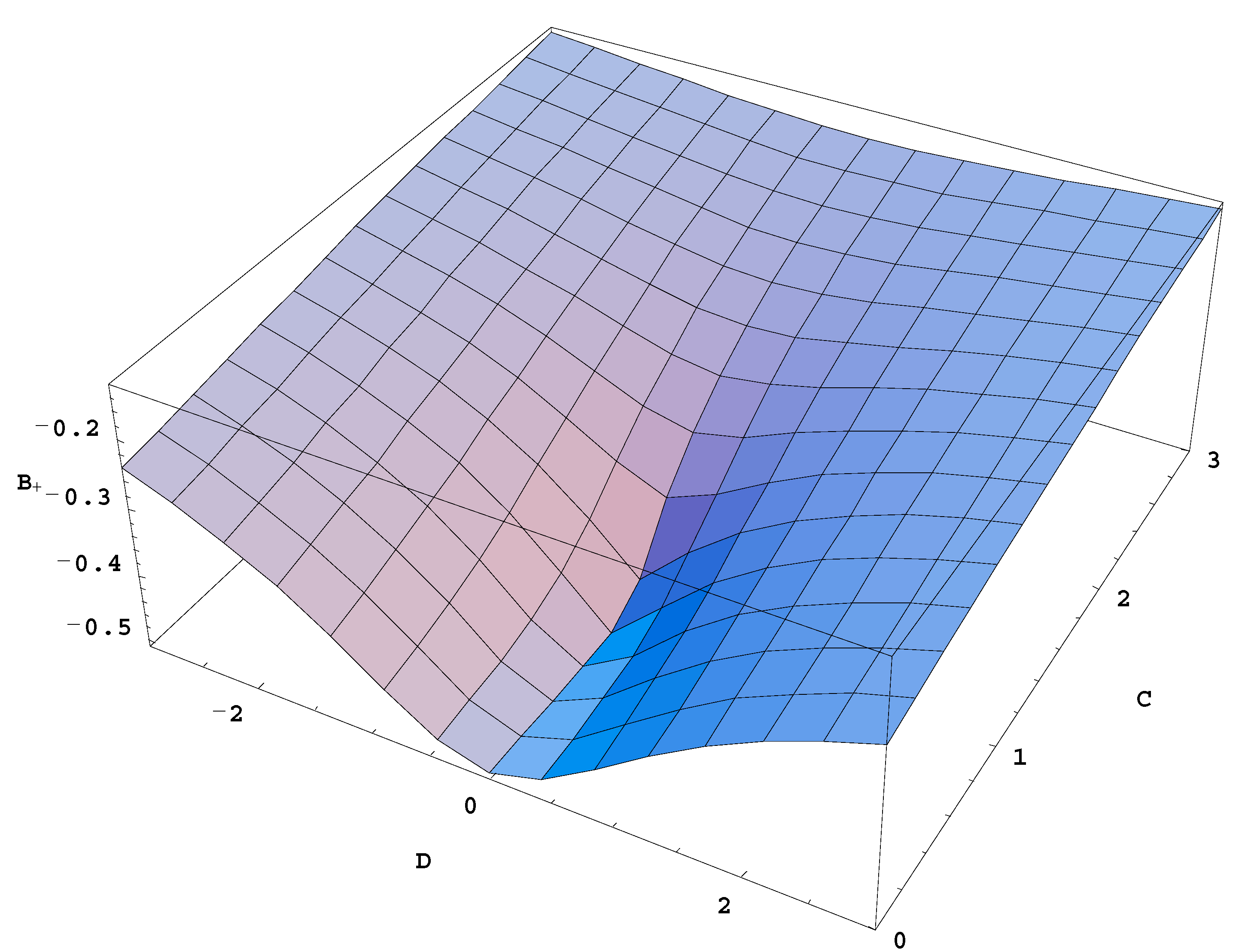
Figure 1 shows a three-dimensional plot of B11+ (denoted in the plot for brevity as B+) versus I22,0/I11,0 (denoted in the plot as C) and I12,0/I11,0 (denoted in the plot as D).
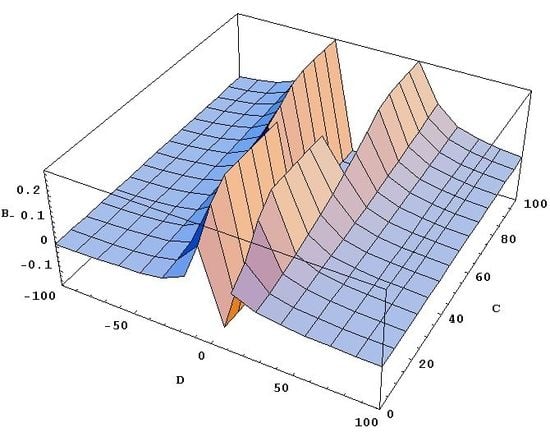
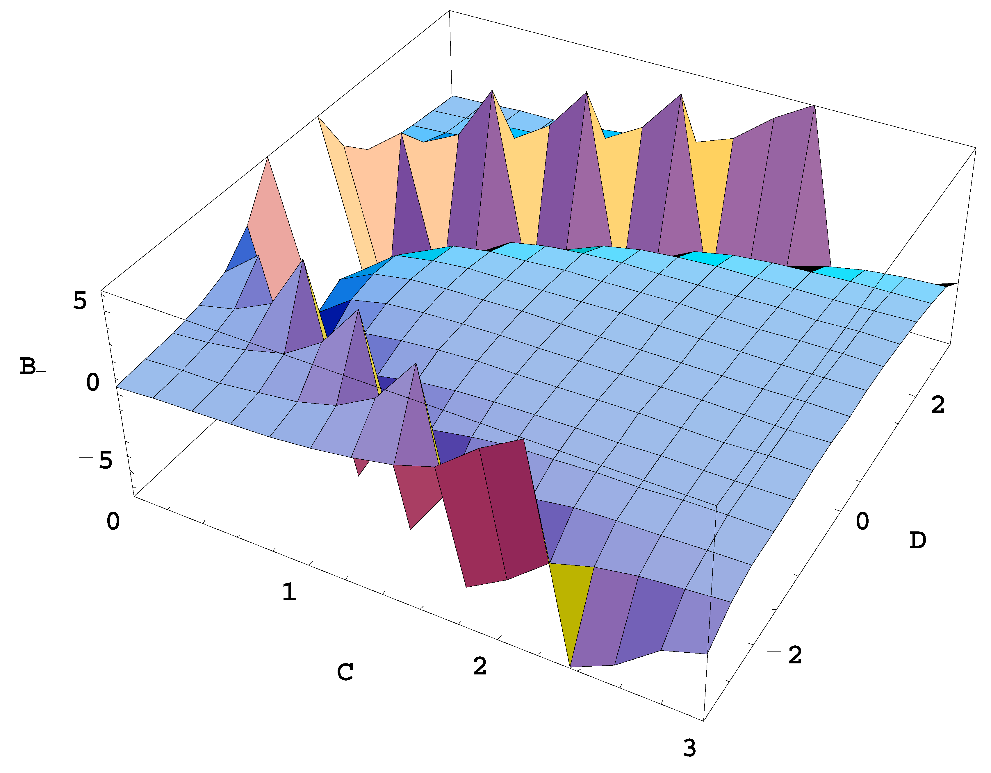
Figure 2 shows a three-dimensional plot of B11– (denoted in the plot for brevity as B–) versus I22,0/I11,0 (denoted in the plot as C) and I12,0/I11,0 (denoted in the plot as D).
Here is an intermediate summary of the above results. By employing the GHD, we have proven the existence of the classical non-radiating states of the charged spherical harmonic oscillator—similarly to the corresponding results of paper [8] for hydrogenic atoms.
Physically, this is the manifestation of a non-Einsteinian time-dilation. Time dilates more and more as the energy of the system becomes closer and closer to the energy of the classical non-radiating state:
t′ = |{1 + I22,0/I11,0 ± [(I22,0/I11,0 − 1)2 + I12,02/I11,02]1/2}B11(E) + 1|t
At the classical non-radiating state, the time gets dilated infinitely. As a result, the frequency of the revolution along an elliptical orbit ωg in Equation (41) vanishes—consequently, the radiation also vanishes.
In the important particular case of I22,0 = I11,0, corresponding to the circular orbits, the above formulas can be simplified as follows. In this case, from Equation (34) follows γ = 0, so that from Equation (35) we get α+ = 1 and α– = −1, as it should be for the circular orbits (see Equation (31)). Then Equation (36) simplifies to
where the plus sign corresponds to α = 1 and the minus sign corresponds to α = −1.
ωg/ω0 = |(2 ± |I12,0|/I11,0)B11(E) + 1|
It is seen that, in this particular case, the generalized frequency ωg vanishes (and so does the radiation) at the following values of B11(E):
and
B11+(Est) = −1/(2 + |I12,0|/I11,0) for α = 1
B11− (Est) = −1/(2 − |I12,0|/I11,0) for α = −1
Obviously, Equation (47) is valid, except if |I12,0|/I11,0 = 2. In the exceptional case, Equation (45) yields a trivial result: ωg = ω0.
The primary result for the circular orbits is non-trivial. Namely, there are classical non-radiating states, corresponding to B11(E) = B11+(Est) for α = 1 or B11(E) = B11−(Est) for α = −1.
Thus, for each direction of the revolution of the charged particle in the orbital plane, there is one value of B11(E)—given by Equations (42) and (43) in the general case of the elliptical orbits or by Equations (46) and (47) for the particular case of the circular orbits—for which the radiation vanishes. The fact that, for each direction of the revolution, there is only one value of B11(E), does not mean that there is only one classical stationary state. Indeed, if the dependence of B11 on the energy E is oscillatory (with the amplitude greater than or equal to the absolute value of the right side of Equation (42) for α = α+, or with the amplitude greater than or equal to the absolute value of the right side of Equation (43) for α = α–), then there would be an infinite number of the energies of the classical stationary states Est—just as in the corresponding quantum solution.
Here is an example, illustrating the statement from the previous sentence for the case of circular orbits—for the subcase of α = 1 chosen for definiteness. Let us consider the following dependence of B11+ on the energy E:
where Est,0 is the energy of the lowest non-radiating state (the ground state) and both E and Est,0 are measured in units of ħω0. In Equation (48), C is a constant, which is an analog of the Maslov index [18], which, for spherically symmetric potentials, is equal to 1/2 (see, e.g., the textbook [19]). With C = 1/2, Equation (48) takes the form
B11+(E) = −|cos[π(E − C)/(Est,0 − C)]|/(2 + |I12,0|/I11,0)
B11+(E) = −|cos[π(E − 1/2)/(Est,0 − 1/2)]|/(2 + |I12,0|/I11,0)
From Equation (49), it is easy to find out that E = Est,n, where
where the quantity B11+ satisfies Equation (46), so that the sequence of values Est,n from Equation (50) is the sequence of the energies of the classical non-radiating stationary states. More explicitly,
Est,n − 1/2 = (n + 1)(Est,0 − 1/2), n = 0, 1, 2, …,
Est,n = (n + 1)Est,0 − n/2
If Est,0 = 3/2, then the sequence of values Est,n from Equation (51) would coincide with the corresponding quantum results.
4. Conclusions
We extended the applications of the GHD to a charged Spherical Harmonic Oscillator (SHO). We demonstrated that, by using the higher-than-geometrical symmetry (i.e., the algebraic symmetry) of the SHO and the corresponding additional conserved quantities, it is possible to obtain classical non-radiating (stationary) states of the SHO. Generally, there is an infinite number of such states of the SHO—just as was the case for hydrogenic atoms, as was shown in paper [8]. Both the existence of the classical stationary states of the SHO and the infinite number of such states are consistent with the corresponding quantum results.
Physically, the existence of the classical stationary states is the manifestation of a non-Einsteinian time-dilation. Time dilates more and more as the energy of the system becomes closer and closer to the energy of the classical non-radiating state.
It should be emphasized that we obtained the above new results from first principles. We did not use any quantization postulates or any input from experiments.
It is worth mentioning that the SHO and hydrogenic atoms are not the only microscopic systems that can be successfully treated by the GHD. Indeed, all classical systems of N degrees of freedom have the algebraic symmetries ON+1 and SUN, and this does not depend on the functional form of the Hamiltonian. In particular, all classical spherically symmetric potentials have algebraic symmetries, namely tO4 and SU3; they possess an additional vector integral of the motion, while the quantal counterpart-operator does not exist [20,21,22]. (This fact was employed in paper [9], where the authors successfully applied the GHD to a modified Coulomb potential.) This offers possibilities that are absent in quantum mechanics, as noted in paper [8].
Since there are lots of classical systems possessing an algebraic symmetry and, therefore, having additional integrals of the motion, as mentioned in the previous paragraph, it should be obvious that the classical systems studied in papers [8,9] and in the present paper do not constitute a comprehensive list. For example, another fundamental physical system—an electron in the field of two stationary nuclei—is a good candidate to be treated by GHD. Indeed, this system has an additional integral of the motion—the projection of the super-generalized Runge–Lenz vector on the internuclear axis, the latter vector being derived in paper [23].
Funding
This research received no external funding.
Conflicts of Interest
The author declares no conflict of interest.
References
- Dirac, P.A.M. Generalized Hamiltonian dynamics. Canad. J. Math. 1950, 2, 129–148. [Google Scholar] [CrossRef]
- Dirac, P.A.M. Generalized Hamiltonian dynamics. Proc. R. Soc. A 1958, 246, 326–332. [Google Scholar] [CrossRef]
- Dirac, P.A.M. Lectures on Quantum Mechanics; Academic: New York, NY, USA, 1964; Reprinted by Dover Publications, 2001. [Google Scholar]
- Sergi, A. Generalized bracket formulation of constrained dynamics in phase space. Phys. Rev. E 2004, 69, 21109. [Google Scholar] [CrossRef] [PubMed]
- Sergi, A. Phase space flows for non-Hamiltonian systems with constraints. Phys. Rev. E 2005, 72, 31104. [Google Scholar] [CrossRef] [PubMed] [Green Version]
- Sergi, A. Non-Hamiltonian commutators in quantum mechanics. Phys. Rev. E 2005, 72, 66125. [Google Scholar] [CrossRef] [PubMed] [Green Version]
- Sergi, A. Statistical mechanics of quantum-classical systems with holonomic constraints. J. Chem. Phys. 2006, 124, 24110. [Google Scholar] [CrossRef] [PubMed] [Green Version]
- Oks, E.; Uzer, T. Application of Dirac’s generalized Hamiltonian dynamics to atomic and molecular systems. J. Phys. B At. Mol. Opt. Phys 2002, 35, 165–173. [Google Scholar] [CrossRef]
- Camarena, A.; Oks, E. Application of the generalized Hamiltonian dynamics to a modified coulomb potential. Int. Rev. At. Mol. Phys. 2010, 1, 143–160. [Google Scholar]
- Oks, E. Breaking Paradigms in Atomic and Molecular Physics; World Scientific: Singapore, 2015. [Google Scholar]
- Goedecke, G.H. Classically radiationless motions and possible implications for quantum theory. Phys. Rev. 1964, 135, B281–B288. [Google Scholar] [CrossRef]
- Raju, C.K. The Electrodynamic 2-body problem and the origin of quantum mechanics. Found. Phys. 2004, 34, 937–962. [Google Scholar] [CrossRef] [Green Version]
- Puthoff, H.E. Ground state of hydrogen as a zero-point-fluctuation-determined state. Phys. Rev. D 1987, 35, 3266–3269. [Google Scholar] [CrossRef] [PubMed]
- Cole, C.D.; Zou, Y. Quantum mechanical ground state of hydrogen obtained from classical electrodynamics. Phys. Lett. A 2003, 317, 14–20. [Google Scholar] [CrossRef] [Green Version]
- Nieuwenhuizen, T.M. On the stability of classical orbits of the hydrogen ground state in stochastic electrodynamics. Entropy 2006, 18, 135. [Google Scholar] [CrossRef] [Green Version]
- Landau, L.D.; Lifshitz, E.M. Mechanics; Pergamon Press: Oxford, UK, 1960. [Google Scholar]
- Landau, L.D.; Lifshitz, E.M. Classical Theory of Fields; Pergamon Press: Oxford, UK, 1960. [Google Scholar]
- Mukunda, N. Dynamical symmetries and classical mechanics. Phys. Rev. 1967, 155, 1383–1386. [Google Scholar] [CrossRef]
- Bacry, H.; Ruegg, H.; Souriau, J.M. Dynamical groups and spherical potentials in classical mechanics. Commun. Math. Phys. 1966, 3, 323–333. [Google Scholar] [CrossRef]
- Fradkin, D.M. Existence of the dynamic symmetries O4 and SU3 for all classical central potential problems. Progr. Theor. Phys. 1967, 37, 798–812. [Google Scholar] [CrossRef] [Green Version]
- Maslov, V.P.; Fedoriuk, M.V. Semi-Classical Approximation in Quantum Mechanics; Springer: Berlin, Germany, 1981. [Google Scholar]
- Landau, L.D.; Lifshitz, E.M. Quantum Mechanics; Pergamon Press: Oxford, UK, 1965. [Google Scholar]
- Kryukov, N.; Oks, E. Super-generalized Runge-Lenz vector in the problem of two coulomb or newton centers. Phys. Rev. A 2012, 85, 54503. [Google Scholar] [CrossRef]
Figure 1.
Three-dimensional plot of B11+ (denoted in the plot for brevity as B+) from Equation (42) versus I22,0/I11,0 (denoted in the plot as C) and I12,0/I11,0 (denoted in the plot as D).
Figure 1.
Three-dimensional plot of B11+ (denoted in the plot for brevity as B+) from Equation (42) versus I22,0/I11,0 (denoted in the plot as C) and I12,0/I11,0 (denoted in the plot as D).

Figure 2.
Three-dimensional plot of B11– (denoted in the plot for brevity as B–) from Equation (43) versus I22,0/I11,0 (denoted in the plot as C) and I12,0/I11,0 (denoted in the plot as D).
Figure 2.
Three-dimensional plot of B11– (denoted in the plot for brevity as B–) from Equation (43) versus I22,0/I11,0 (denoted in the plot as C) and I12,0/I11,0 (denoted in the plot as D).

© 2020 by the author. Licensee MDPI, Basel, Switzerland. This article is an open access article distributed under the terms and conditions of the Creative Commons Attribution (CC BY) license (http://creativecommons.org/licenses/by/4.0/).
Share and Cite
MDPI and ACS Style
Oks, E. Application of the Generalized Hamiltonian Dynamics to Spherical Harmonic Oscillators. Symmetry 2020, 12, 1130. https://0-doi-org.brum.beds.ac.uk/10.3390/sym12071130
AMA Style
Oks E. Application of the Generalized Hamiltonian Dynamics to Spherical Harmonic Oscillators. Symmetry. 2020; 12(7):1130. https://0-doi-org.brum.beds.ac.uk/10.3390/sym12071130
Chicago/Turabian StyleOks, Eugene. 2020. "Application of the Generalized Hamiltonian Dynamics to Spherical Harmonic Oscillators" Symmetry 12, no. 7: 1130. https://0-doi-org.brum.beds.ac.uk/10.3390/sym12071130
Note that from the first issue of 2016, this journal uses article numbers instead of page numbers. See further details here.