Real-Time Data Filling and Automatic Retrieval Algorithm of Road Traffic Based on Deep-Learning Method


School of Traffic and Transportation, Beijing Jiaotong University, Beijing 100044, China
*
Author to whom correspondence should be addressed.
Symmetry 2021, 13(1), 1; https://0-doi-org.brum.beds.ac.uk/10.3390/sym13010001
Submission received: 13 October 2020
/
Revised: 8 December 2020
/
Accepted: 12 December 2020
/
Published: 22 December 2020
(This article belongs to the Special Issue Mathematical Modeling and Computational Methods in Science and Engineering III)
Abstract
:In order to enhance the real-time and retrieval performance of road traffic data filling, a real-time data filling and automatic retrieval algorithm based on the deep-learning method is proposed. In image detection, the depth representation is extracted according to the detection target area of a general object. The local invariant feature is extracted to describe local attributes in the region, and it is fused with depth representation to complete the real-time data filling of road traffic. According to the results of the database enhancement, the retrieval results of the deep representation level are reordered. In the index stage, unsupervised feature updating is realized by neighborhood information to improve the performance of a feature retrieval. The experimental results show that the proposed method has high recall and precision, a short retrieval time and a low running cost.
1. Introduction
With the rapid development of the economy, urban population and vehicle ownership are growing rapidly, traffic flow is increasing, and congestion is becoming more and more serious. In order to reduce traffic pressure, the most important thing is to accurately count the traffic flow to achieve a reasonable diversion. To achieve this goal, real-time data filling and the automatic retrieval of road traffic has become a crucial step [1,2]. In addition, in recent years, the increase of road-monitoring cameras has also provided hardware conditions for vehicle detection. Therefore, it is of great practical significance to study the technology of the real-time automatic detection of vehicles by surveillance video and improve its retrieval accuracy. In the early days, the Traffic Management Department mainly used manual discrimination methods to identify the traffic status and monitored the road conditions through manual patrols and citizen reports. Later, with the rapid development of social economy and the rapid increase in the number of motor vehicles, road conditions became intricate and complicated. Manual discrimination methods can no longer meet the demand for the real-time discrimination of traffic conditions. Many domestic and foreign researchers have begun to study advanced technologies. It is an automatic identification method for the means and, finally, has achieved good results in practical applications.
Traditional methods have made great progress in video surveillance image processing, but the interference of background and light; the influence of bad weather such as rain, snow, and night; and the problem of vehicle overlap in video surveillance images are still not effective, and how time-consuming traditional methods are is too long to meet real-time needs. As one of the hottest technologies, deep-learning technology has shown amazing abilities in many fields. Using a convolution neural network to detect images is a great application of deep learning in image processing. At present, relevant experts have given some good research results; for example, Wang Xinlong proposed an image retrieval algorithm based on depth learning, which mainly uses the response values of different layers in the multi-layer depth network model as the feature expression of the image and uses the depth learning model to carry out image retrieval research. Ren Xiali et al. put forward an image retrieval algorithm based on deep-learning features. Using a convolution neural network, image features are extracted based on deep learning. By analyzing the correlations of the features, the principal component analysis algorithm is used to reduce the dimensions of the features and reduce the loss of information as much as possible. On this basis, the features are hashed, and coding is used to do a fast image retrieval. Ma Dongmei also proposed an image retrieval algorithm based on depth learning, which mainly highlighted the importance of feature learning through the depth of a neural network. Although the above methods achieved very satisfactory research results, there were still some deficiencies, which need to be further improved. On the basis of traditional methods, this paper designs and proposes a real-time data filling and automatic retrieval algorithm based on the deep-learning method. This paper proposes a road extraction model based on a deep-learning network that not only greatly improves the accuracy of image road extraction but, also, greatly enhances the fitness of the same model for road extraction in different terrain environments. The general object detector is used to detect the object of interest in the image to eliminate the interference of the background area and to overcome the changes of the image content in the spatial layout and angle of view. The depth representation is extracted from these target areas, and the local significant areas in the target are described by an effective local feature aggregation method, and the early fusion technique of the feature level is used to express the target area in a very efficient and compact manner. In the large-scale image retrieval application, a small number of object-level representations in the image are indexed by an inverted structure, and the features are compressed by product quantization so as to achieve an accurate, efficient, and economical retrieval system.
2. Algorithm
2.1. Data Missing Mechanism
There are many reasons for missing data, and the types of data missing are also different. Mastering the data missing mechanism is a prerequisite for research work. In 1976, Little and Rubin clarified the data missing mechanism and divided the data missing into three categories.
(1) Missing completely at random (MCAR)
For the data set, assumes that the attribute is missing, represents the missing state of , a value of 1 indicates that the data is complete, and a value of 0 indicates that the data is missing. The absence of has nothing to do with itself and has nothing to do with the other attributes. This situation is completely missing at random, which can be expressed by Formula (1).
(2) Missing at random (MAR)
Missing at random weakens the hypothesis of missing completely at random. The missing data in the dataset is related to other data in the dataset, not to itself. Therefore, random deletion can be regarded as a general form of completely random deletion, which can be expressed by Formula (2).
(3) Missing at Nonrandom (MNAR)
Data that is not randomly missing has a relationship with its own characteristics and has no relationship with other attributes in the dataset. In the traffic system, the cause of the MNAR is the failure of the traffic detector. In this study, because the experimental data assumes that the detector is normal, the factor of the detector failure is not considered. This part of the data can be eliminated by Formula (3).
2.2. Data Missing Processing Method
Missing data has always been a very common problem. Incomplete data information can cause research work to be blocked or even collapse; especially when the amount of data is small, the processing of missing data is crucial to research work. Scholars at home and abroad have done a lot of research on the processing of missing data. Our research only considers filling processing and does not discuss nonprocessing and deleting operations. The following is an introduction and analysis of widely used filling processing methods.
(1) Artificial filling method
Filling is done by the person who knows the missing data best, and the data obtained has the least deviations. From the effect point of view, it is the best filling method. However, it is time-consuming and inefficient, especially in the current era of data explosion; in the face of huge amounts of data and a large number of vacancies, this method is not feasible and expensive.
(2) Special value filling method
Considering the waste of data volume caused by the deletion method, the null value is treated as a special attribute value. In most database processing, the null value is often filled with “unknown” or “null”. Although the amount of data is guaranteed, it may cause data deviation and create new problems, especially when these missing data are very important attributes.
(3) Mean Fill Method
When the data attributes are more important and the amount of data is huge, it is difficult to use manual filling and special value filling; then, the mean value filling method can be used. According to the type of the dataset attribute, the data can be divided into continuous data and discrete data and processed separately. If the missing data is continuous, the average value of other attributes in the dataset where the attribute is located is used for filling; if the missing data is discrete, then according to statistical principles, the value of the attribute with the most values in other states is used as the filling value. The best application scenario of this method is that the data is normally distributed, but this method will produce biased estimates, and in actual use, it is difficult for researchers to determine the data distribution, so it should be carefully considered when using it.
(4) Return to fill
The regression filling method uses the quantitative relationship between two or more attributes to establish a statistical regression model to calculate the estimated value of the attribute, and the estimated value is used as the filling value of the missing data. This method can not only deal with the lack of a single attribute but, also, the situation where multiple attribute values are missing, but the construction of the model and the determination of the parameters require a lot of time and calculation costs, and a sufficient amount of known data is required for model selection confirmation. Therefore, only very important tasks are used to regress and fill.
2.3. Real-Time Data Filling of Road Traffic
A convolutional neural network is an important branch of the deep-learning network. A convolutional neural network is especially good at image processing, because it is a very effective structure that can extract all kinds of information of images very well [3,4]. A convolutional neural network is a special neural network structure with grid information data. Generally, when the deep-learning network model uses the convolution structure instead of the common matrix operation structure, it is called a convolution neural network.
This paper uses a convolutional neural network to realize the real-time data filling of road traffic. The flow chart of the pooling operation calculations of the convolutional neural network is shown in Figure 1.
In Figure 1, R represents register data. It can give full play to the computing power of the deep convolutional neural network model and greatly improve its efficiency. The task object of the pooling unit is the result of the convolution layer after activation processing. The maximum or average value is output through the pooling operation, which is passed to the next layer to continue to complete the pooling operation. Convolution computation is complicated, while pooling is relatively simple. Therefore, most networks are implemented by pooling.
Convolution is a common mathematical operation, and the most widely used field is signal analysis and automatic control. The following is the mathematical definition of the convolution operation of a one-dimensional continuous signal:
where represents the membership function of the -th data object of the traffic signal, and represents the Euclidean distance from the data object to the -th cluster center. The convolution operations for discrete signals are:
In the application of machine learning, the input is usually a high-dimensional data array, also known as a tensor. When the variable is two-dimensional, the discrete convolution is extended to:
where represents the membership matrix, and represents the cluster center. Convolution improves the deep-learning system by three features, which are
- (1)
- sparse interactions,
- (2)
- parameter sharing, and
- (3)
- equivariant representation.
The traditional neural network uses matrix multiplication to establish the connection between input and output. Each independent parameter of the parameter matrix describes the interaction between each input unit and each output unit. This means that each output unit interacts with each input unit. However, the convolutional neural network is characterized by sparse interaction (also known as sparse connectivity or sparse weight). This is achieved by making the size of a core much smaller than the size of the input. For example, when performing image processing, the input image may contain millions of pixels, but small, meaningful features, such as image edges, can be detected by using only cores that occupy tens to hundreds of pixels. This means less model parameters need to be stored, which can not only reduce the storage requirements of the model but, also, improve the statistical efficiency. This also means that less computations are needed to get the output. These efficiency improvements are often important for video or video tasks. In the deep convolution network, the deep element may not be directly connected to most of the inputs.
A full convolution deep-learning network can effectively transform from image to image [5,6]. By applying the full convolution deep-learning network to real-time data filling and the automatic retrieval of road traffic based on the deep-learning method, the real-time data prediction model of road traffic based on the deep-learning method can be realized. A real-time data prediction model for road traffic is a more direct method of deep-learning road extraction, which realizes the leap of road extraction results in images directly from the input network model of high-resolution remote sensing images.
The function of a deconvolution layer is a kind of up-sampling method, which can increase the size of the input feature map. The operation of deconvolution can be equivalent to adding a pixel with a value of zero between the input feature pixels and then performing the conventional convolution operation so the input feature image is used to complete the up-sampling operation of the feature image by a convolution operation [7].
The relevant parameters of the deconvolution operation are set to ensure that the length and width of the feature image are doubled when each deconvolution operation is carried out, so that it forms a symmetrical structure with the feature extraction structure layer.
The biggest disadvantage of the original full convolution network is that it can only locate the approximate position of the object in the image, and the details of the edge of the object are fuzzy. This is not good for road extraction of high-resolution remote-sensing images, because, in the high-resolution remote-sensing image, the low-level roads are all the details of the image, and the proportions in the image are very small. The structure of the original FCN (fully convolutional network) is difficult to extract the low-level road. In order to extract the low-level road from the original image, this paper makes the following improvements on the basis of the FCN:
(1) Increasing the connection between peer-to-peer networks.
According to the understanding of this paper, the function of the front part of the full convolution network is image feature decomposition, the function of the middle part is feature transformation, and the function of the back part is image feature reconstruction. The structure of the whole network should be a symmetrical structure, but the original FCN does not do so, not a symmetrical structure.
(2) The number of features in the peer layer is consistent.
In the original FCN, because the number of features in the image feature decomposition layer is not equal to the number of features in the image reconstruction layer, the FCN author makes the number of image features equal to the number of output features after the convolution feature extraction operation on the feature decomposition layer [8,9] and then establishes the connection between the feature decomposition and the feature reconstruction through the addition operation.
In this paper, the redesign of the real-time data prediction model for road traffic based on deep learning is to keep the same number of features in image feature decomposition and image feature reconstruction, so that the relationship between all peer layers can be established directly.
In order to make the designed deep-learning model applicable in practice [10], it must be trained and studied before application. A network model initialized randomly is meaningless. The first step of training a neural network is to acquire and make datasets for training and testing.
The deep-learning model of this paper needed to solve the problem of automatic road extraction from high-resolution optical remote-sensing ortho images. Therefore, the input of the neural network model was naturally the high-resolution optical ortho images. Since the original remote-sensing images were huge and the computer computing resources were limited, it could not be directly input into the neural network for training, so the original high-resolution remote-sensing images needed to be stored in blocks first. The work of block storage can be realized by programming using Envi, GDAL, MATLAB, and other image-processing platforms.
After the block processing, the original images of the training dataset were obtained. The next step was to mark the road in the remote-sensing images and get the corresponding marked images as the goal of the fully supervised learning [11,12]. The collection and marking of training database data in deep learning has always been a difficult problem for researchers and users of deep learning. To solve this problem, there are various open-training databases for researchers to use. However, for this problem, these databases were not suitable. The training data of this paper was a high-resolution optical remote-sensing image; the data source can be downloaded and purchased from the network, but the data annotation is a huge workload and boring work that needs a lot of time. The convenience and flexibility of data annotation tools determine the accuracy and efficiency of data annotation. In this paper, a software tool for road extraction and annotation of the remote sensing image was specially designed for the problem of data annotation.
The formula of the ultimate performance of the model can be obtained through the analysis
where represents the fuzzy weighted index. Based on the above analysis, local invariant features were extracted and fused with the depth representation to complete the real-time data filling of road traffic.
2.4. Real-Time Data Filling and the Automatic Retrieval Algorithm of Road Traffic
As in Section 2.3, the same global feature extraction method based on depth representation [13,14] was used as the original data feature expression. Specifically, for a piece of data to be extracted, input it into a convolutional neural network model (AlexNet model) pretrained on the classification task and use the network response of the middle layer as the data feature. In the following research, the following two characteristics were tested:
(1) 256 dimensional layer output features.
The same settings as in Section 2.2 were used, which did not change the aspect ratio of the traffic data, and took a mean value for each channel of the response to the layer.
(2) 4096 dimensional Fc7 layer output features.
The database of traffic data retrieval is set as , where is the feature expression vector of the -th database traffic data, and is the size of the database. Given a query image , the similarity calculation of with respect to the database traffic data is as follows:
since all image features were normalized; namely,
In the query stage, the original traffic data features are used to perform an initial retrieval operation [15], and some of the database traffic data with the highest rankings are defined as the neighborhood of the query traffic data, expressed as . Then, one or more anchors are calculated in the neighborhood, expressed as
where M is the number of anchors. Then, the query traffic data feature and the database traffic data in the neighborhood are represented as the residual vector relative to the anchor point, and the similarity between them will be recalculated through the cosine distance between the residual vectors [16,17]. Finally, through the similarity of the new calculations, the image in the neighborhood is reordered to get the final retrieval results.
In the field of the nearest neighbor search, there are two most popular neighborhood definition methods: k-neighborhood and ∈-neighborhood. In high-dimensional feature space, the k-neighborhood is defined as k feature points closest to the query feature, while ∈-neighborhood is defined as all feature points whose distance from the query feature are not greater than ∈. Since the cosine distance is used to measure the feature distance [18,19], ∈ is defined as the minimum similarity between the feature distance and query feature distance in a neighborhood.
Obviously, the k-neighborhood considers a fixed number of features, regardless of the local distribution of those features near the query traffic data features, while the ∈-neighborhood considers the fixed range of the neighborhood near the query features, regardless of the number of feature points to be introduced, so the number of features in the neighborhood can be adaptively selected according to the feature density near the query features.
The definition of the anchor point aims to make the generated residual vector contain useful information to the maximum extent and improve the retrieval performance [20]. This goal is not easy to achieve, because monitoring information is not available. However, the context dissimilarity measure mentioned in the relevant reference hopes that the local residual expression can improve the symmetry of the neighboring relationship between the features in the neighborhood; that is, the related image features can become the neighborhood features of each other at the same time.
Intuitively speaking, a very direct anchor setting method is to set it as the mean vector of all features in the neighborhood, including query features, so that the anchor will be closer to the clustered feature points and make the distribution of features more uniform when the cosine distance is used to measure the similarity of the residual vectors [21]. Similarly, the anchor can be set as the median vector of these eigenvectors, so it is expected to eliminate the influence of abnormal eigenvector points around the query features. These two anchor calculation methods are, respectively, expressed as and .
In order to consider more detailed residual information, more than one anchor point is used to express the residual of the feature vector. In this way, each feature vector in the query feature neighborhood is spliced by its residual vectors about all anchors. Specifically, if there are multiple anchors , the residual vector of the query feature or database traffic data feature 2 can be calculated as
where the symbol ⊕ represents the splicing operation of the vectors. The normalization is performed on each segment of the stitched feature vector, so the similarity between the two residual feature vectors and can be directly obtained by the inner product operation , which is equivalent to the sum of the cosine distance of each segment of the feature. Obviously, the more anchors are used, and the more feature dimensions will be obtained.
The algorithm is used to calculate clustering centers for the features in the neighborhood, which are used as anchor points to represent the more detailed local feature distribution. This method of calculating multiple anchors is called . It is noted that, when , this expression degenerates to the method mentioned earlier.
The nonsimilarity measure of the context is an effective method to improve the feature distance measures by using the local distribution of the feature spaces. In this method, each image feature in the database is assigned a neighborhood distance factor, which is used to represent the average distance between the feature and the feature in its neighborhood. It is defined as
where is the -nearest neighbors of feature . Then, the distance between the query traffic data feature and database image feature is calculated by the following formula:
where is Euclidean distance; that is:
In the initial query stage, the neighborhood distance factor is calculated by the original eigenvector, while, in the reorder stage, the factor is calculated by the normalized residual vector.
In addition to considering the neighborhood of query traffic data features, a very intuitive extension is to also use its neighborhood local residual expression for each feature in the database traffic data and query it in the query stage. The characteristics of the traffic flow data are also expressed accordingly, and stronger constraints are used to improve the accuracy of the feature matching. That is, different traffic flow data needs to have sufficient similarity in their respective local residual expressions. The above method is a database supplement.
Specifically, if an anchor is calculated in the neighborhood of the query traffic data features and an anchor is calculated in the neighborhood of the database traffic data features, then there are two local residual expressions about anchor , respectively:
The local residual calculation formula of the anchor point is as follows:
The distance calculation formula for features and can be expressed in the following forms:
This matching score considers that two features to be compared need to have enough similarity in their respective local neighborhood distributions. In the formula, the two scores are integrated by adding instead of multiplying, because their values may be negative. In the algorithm, the process of using a database supplementary method to search is summarized.
In general, considering a larger neighborhood, it can get a higher recall rate when reordering, but it may lose the local feature distribution information around the query feature to some extent. Next, the performance of the image retrieval in a different neighborhood is tested.
In this section, database enhancement and query results reordering are carried out at the depth representation level, and the retrieval performance is enhanced with minimal computation and storage costs at the offline index stage and online query stage, respectively. In the index stage, the unsupervised feature updating is realized by using the relationship between database traffic data and neighborhood information, which makes the obtained features have a better real-time performance of road traffic data retrieval.
3. Simulation Experiment
In order to verify the comprehensive effectiveness of the proposed real-time data filling and automatic retrieval algorithm for road traffic based on the deep-learning method, simulation experiments are needed. The experimental environment is Intel(R) Pentium(R)4, CPU 2.30 GHz, 2 GB of memory, and the operating system Microsoft Windows 7 (64 bit).
(1) Traffic data filling results
In order to more intuitively show the error of the filling model under different missing rates, a histogram of the MAE (Mean Absolute Error, It represents the average of the absolute deviations of all individual observations from the arithmetic mean), MSE (Mean Squared Error, The mean square error is the expected value of the square of the difference between the estimated and true values of the parameter), and RMSE (Root Mean Square error, It is the square root of the square root of the deviation between the observed value and the truth value and the ratio of the observed times) is drawn. The MAE histogram of the filling model under different missing rates is shown in Figure 2.
From the error statistics under different missing rates and the MAE histogram, it can be seen that, as the missing rate increases, the accuracy of the filling decreases, but the fluctuation is small and relatively stable. The minimum value of the MAE was obtained when the missing rate was 15%, which was 8.559, and the maximum value was obtained when the missing rate was 45%, which was 10.365. The average MAE under different missing rates was 9.261.
The MRE histogram of the filling model under different missing rates is shown in Figure 3.
From the error statistical results under different missing rates and the histogram of the MRE, it can be seen that the filling model is stable. The minimum value of the MRE is obtained when the missing rate is 10%, which is 0.169, and the maximum value is obtained when the missing rate is 50%, which is 0.213, and the average MRE under different deletion rates is 0.181.
The RMSE histogram of the filling model under different missing rates is shown in Figure 4.
From the error statistics results under different missing rates and the histogram of the RMSE, it can be seen that, as the missing data increases, the overall performance of the model is stable. When the missing rate is 15%, the RMSE achieves a minimum value of 11.936. When the missing rate is 50%, the RMSE achieves a maximum of 15.608.
(2) Missing data filling effect
In order to measure the performance of the filling model proposed in this article, this section compares the filling method based on deep learning with the historical average and neural network. The historical average is the most basic method of filling missing data. The neural network processes nonlinear data. Higher accuracy is a more advanced technology. The trained model is used to fill in the missing data of the traffic flow, and the statistical results of the three evaluation indicators of the filling results are shown in Table 1.
It can be seen from the comparison of the deep-learning and historical average methods, neural network methods in filling results under different missing rates, and the comparison of the MAE, MRE, RMSE histograms drawn from the filling results that, as the missing rate increases, the error of the filling model appears. On the upward trend, the historical average method and deep-learning method are relatively stable, but the historical average method has a low filling accuracy, while the neural network method fluctuates greatly. On the whole, the filling results of deep learning are significantly better than the historical average and neural network methods.
Figure 5 shows the filling effect of one week of traffic flow data when the missing data of the method based on deep learning fills up the missing traffic flow when the missing rate is 20%, which shows the data filling effect more clearly.
Analyzing Figure 5, it can be seen that the method in this paper can effectively fill the missing data of traffic flow with a 20% missing rate.
(3) Retrieval effect comparison
In order to verify the effectiveness of the proposed algorithm, two indexes are selected as evaluation indexes—namely, recall and precision. The comparison results of the recall and precision of different algorithms are given in the table below. The recall rates of different methods are shown in Table 2.
According to Table 2, the recall of different algorithms is different. When the number of the hidden layer nodes is 50, the recall rate of the algorithm in Reference [4] is 95%, the recall rate of the algorithm in Reference [5] is 90%, and the recall rate of the proposed algorithm is 98%. When the number of hidden layer nodes is 300, the recall rate of the algorithm in Reference [4] is 90%, the recall rate of the algorithm in Reference [5] is 88%, and the recall rate of the proposed algorithm is 95%. When the number of hidden layer nodes is 700, the recall rate of the algorithm in Reference [4] is 92%, the recall rate of the algorithm in Reference [5] is 87%, and the recall rate of the proposed algorithm is 97%. The recall rate of the proposed method is always higher, which shows that the retrieval performance of the proposed method is good.
The accuracy change rates of different methods are shown in Table 3.
An analysis of the experimental data in Table 3 shows that, with the continuous increase of the number of hidden layer nodes, the precision rate of various algorithms also changes. When the number of hidden layer nodes is 100, the precision rate of the algorithm in Reference [4] is 92%, that of the algorithm in Reference [5] is 85%, and that of the proposed algorithm is 98%. When the number of hidden layer nodes is 500, the precision rate of the algorithm in Reference [4] is 92%, the precision rate of the algorithm in Reference [5] is 87%, and the precision rate of the proposed algorithm is 99%. When the number of hidden layer nodes is 750, the precision rate of the algorithm in Reference [4] is 92%, the precision rate of the algorithm in Reference [5] is 90%, and the precision rate of the proposed algorithm is 98%.
An analysis of the above two groups of experiments shows that the retrieval effect of the proposed method is the best of the three algorithms.
(4) Retrieval time/(min)
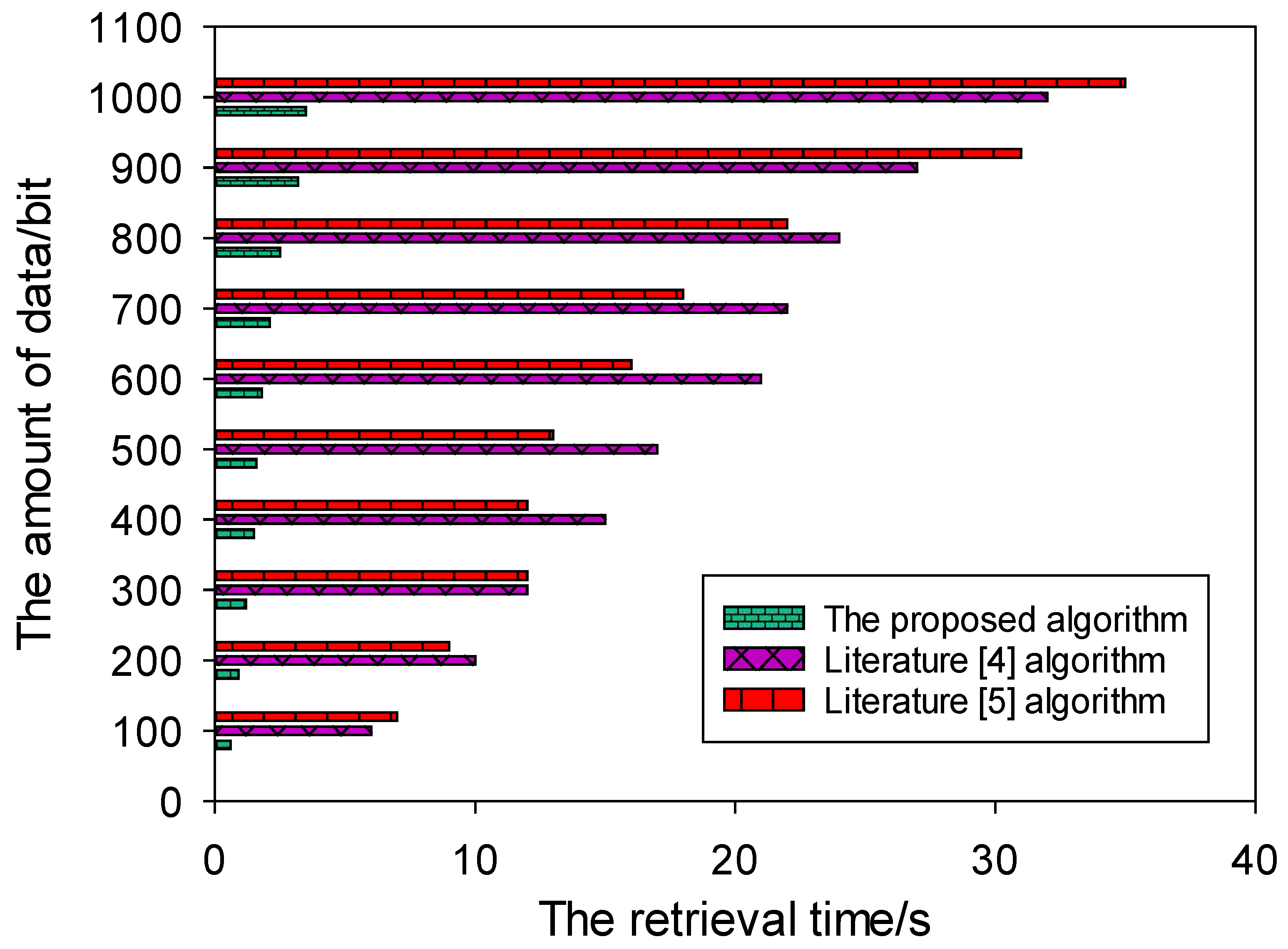
In order to further verify the effectiveness of the proposed algorithm, it needs to compare the retrieval time of the three algorithms as follows, and the specific comparison results are shown in the following figure.
An analysis of the experimental data in Figure 6 shows that the retrieval times of different retrieval algorithms are different under different data amounts. When the amount of data is 200 bits, the retrieval time of the proposed method is 0.9 s, that of the algorithm in Reference [4] is 10 s, and that of the algorithm in Reference [5] is 9 s. When the data volume is 600 bits, the retrieval time of the proposed method is 1.8 s, the retrieval time of the algorithm in Reference [4] is 21 s, and the retrieval time of the algorithm in Reference [5] is 16 s. When the amount of data is 1000 bits, the retrieval time of the proposed method is 3.5 s, the retrieval time of the algorithm in Reference [4] is 32 s, and the retrieval time of the algorithm in Reference [5] is 35 s. According to the overall situation, the retrieval time of the proposed algorithm is the shortest among the three retrieval algorithms, and the retrieval efficiency is the highest.
(5) Operation cost/(10,000 yuan)
The operation costs of the three retrieval algorithms are compared as follows, and the specific comparison results are shown in the Table 4 below.
An analysis of the above experimental data shows that the running cost of different algorithms is different. When the number of experiments is 20, the running cost of the proposed algorithm is 10,500 yuan, that of the algorithm in Reference [4] is 13,800 yuan, and that of the algorithm in Reference [5] is 18,800 yuan. When the number of experiments changes to 50 times, the running cost of the proposed algorithm is 12,600 yuan, the running cost of the algorithm in Reference [4] is 18,600 yuan, and the running cost of the algorithm in Reference [5] is 27,800 yuan. When the number of experiments increases to 80, the running cost of the proposed algorithm is 15,000 yuan, that of the algorithm in Reference [4] is 25,000 yuan, and that of the algorithm in Reference [5] is 36,800 yuan. The operation cost of the proposed method is kept at the lowest throughout the experiment, which shows the superiority of the proposed method.
4. Conclusions
Aiming at the problems of the traditional retrieval methods, such as the long retrieval time, high operation cost, and unsatisfactory retrieval effect, this paper designs and proposes a real-time data filling and automatic retrieval algorithm based on the deep-learning method and obtains the following conclusions:
- (1)
- The automatic extraction of road information from images has been proposed by many methods, but at present, the accuracy of these methods for image road extraction and the adaptability of road extraction in different terrain environments are not very high, which cannot meet the needs of practical application. This paper proposes a road extraction model based on a deep-learning network that not only greatly improves the accuracy of image road extraction but, also, greatly enhances the adaptability of the same model for road extraction in different terrain environments.
- (2)
- The general object detector is used to detect the interesting objects in the image in order to eliminate the interference of the background area, as well as to overcome the changes of the image contents in the spatial layout and perspective scales. In these target regions, the depth representation is extracted, the local significant regions are described through the effective local feature aggregation method, and the early fusion technology of the feature level is used to express the target region very effectively and compactly. In large-scale image retrieval applications, a small number of target-level representations in the image are indexed by an inverted structure, and the product quantization method is used for feature compression to achieve an accurate, efficient, and economic retrieval system.
- (3)
- It focuses on how to further improve the retrieval performance in the representation layer after obtaining the depth representation of the image. In this stage, two effective methods are proposed to enhance the retrieval performance by using the relevant information between the database image features starting from the offline index stage and the online query stage.
Author Contributions
Conceptualization, J.Z.; Data curation, W.X. All authors have read and agreed to the published version of the manuscript.
Funding
This research was supported by the National Natural Science Foundation of China General Projects Grants Nos. 61672002 and 41701120.
Conflicts of Interest
The authors declare no conflict of interest.
References
- Hong, Y.F.; Wei, B.Z.; Liu, C.; Han, Z.Y.; Li, T.Y. Deep multi-level study of foraminal stenosis based on deep learning. J. Intell. Syst. 2019, 14, 708–715. [Google Scholar]
- Yang, J.S.; Yang, Y.N.; Li, T.J. Traffic sign recognition algorithm based on deep separable convolution. LCD Disp. 2019, 34, 1191–1201. [Google Scholar]
- Han, L.Y.; Huang, Y.Z.; Dou, H.R.; Bai, W.J.; Liu, Q. Deep segmentation of left atrial appendage in ultrasound images based on deep learning. Comput. Appl. 2019, 39, 3361–3365. [Google Scholar]
- Liu, F.; Li, G.; Hu, X.; Jin, Z. Research Progress on Program Understanding Based on Deep Learning. Comput. Res. Dev. 2019, 56, 1605–1620. [Google Scholar]
- Guo, M.Z.; Wang, P.Y.; Zhao, L.L. Travel pattern recognition method based on deep learning. J. Harbin Inst. Technol. 2019, 51, 1–7. [Google Scholar]
- Hu, Z.P.; Diao, P.C.; Zhang, R.X.; Li, S.F.; Zhao, M.Y. Attention mechanism based time-group deep network behavior recognition algorithm. Pattern Recognit. Artif. Intell. 2019, 32, 892–900. [Google Scholar]
- Luo, H.B.; Xu, L.Y.; Hui, B.; Chang, Z. Research Status and Prospect of Target Tracking Methods Based on Deep Learning. Infrared Laser Eng. 2017, 46, 14–20. [Google Scholar]
- Li, Y.; Luo, Z.G.; Guan, N.Y.; Yin, X.Y.; Wang, B.; Bo, X.C.; Li, F. Application of deep learning methods in biomedical data analysis. Adv. Biochem. Biophys. 2016, 43, 472–483. [Google Scholar]
- Zuo, P.F.; Hua, Y.; Xie, X.F.; Hu, X.; Xie, Y.; Feng, D. A secure encryption method for deep learning accelerators. Comput. Res. Dev. 2019, 56, 1161–1169. [Google Scholar]
- Yan, W.; Jin, W.; Fu, R.D. Image retrieval combining vlad features and sparse representation. Telecommun. Sci. 2016, 32, 80–85. [Google Scholar]
- Wang, H.Q.; Nie, Z. Application of fast search density peak clustering in image retrieval. Comput. Eng. Des. 2016, 37, 3045–3050. [Google Scholar]
- Zhou, Y.; Zeng, F.Z. Image retrieval algorithm based on two-dimensional compressed sensing and layered features. Chin. J. Electron. 2016, 44, 453–460. [Google Scholar] [CrossRef]
- Li, L.; Feng, L.; Wu, J.; Liu, S.L. Image retrieval based on semi-circular local binary pattern structure correlation descriptors. J. Dalian Univ. Technol. 2016, 56, 532–538. [Google Scholar]
- Gong, Z.T.; Chen, G.X.; Ren, X.L.; Cao, J.S. Image retrieval method based on convolutional neural network and hash coding. J. Intell. Syst. 2016, 11, 391–400. [Google Scholar]
- Li, Z.G.; Hu, D.Y.; Li, J.H.; Cen, J. Content-based remote sensing image database urban area retrieval. Remote Sens. Land Resour. 2016, 28, 67–72. [Google Scholar]
- Duan, Y.J.; Lv, Y.S.; Zhang, J.; Zhao, X.L.; Wang, F.Y. Current Status and Prospects of Deep Learning in the Control Field. J. Autom. 2016, 42, 643–654. [Google Scholar]
- Guo, L.; Gao, H.; Zhang, Y.W.; Huang, H.F. Research on bearing state recognition based on deep learning theory. Vib. Shock 2016, 35, 166–170. [Google Scholar]
- Chen, D.J.; Zhang, W.S.; Yang, Y. Detection and recognition of high-speed railway catenary locator based on deep learning. J. Univ. Sci. Technol. China 2017, 47, 320–327. [Google Scholar]
- Zhao, D.D.; Pan, X.; Liu, X.; Gao, X. Palmprint recognition based on lifting wavelet and deep learning. Comput. Simul. 2016, 33, 338–342. [Google Scholar]
- Fabio, A.; Giovanni, P.; Alessandro, S. V2X Communications Applied to Safety of Pedestrians and Vehicles. J. Sens. Actuator Netw. 2019, 9, 3. [Google Scholar]
- Arena, F.; Pau, G.; Severino, A. An Overview on the Current Status and Future Perspectives of Smart Cars. Infrastructures 2020, 5, 53. [Google Scholar] [CrossRef]
Figure 1.
Flow chart of the pooling operation calculations of the convolutional neural network.

Figure 2.
MAE of the imputation results under different missing rates.

Figure 3.
MRE of the imputation results under different missing rates.

Figure 4.
RMSE of the imputation results under different missing rates.

Figure 5.
Traffic flow series after imputation under a 20% missing rate.

Figure 6.
Comparison results of the retrieval time of different retrieval algorithms.


Table 1.
Comparison of the model imputation results under different missing rates.
| Missing Rate (%) | MAE | MRE | RMSE | ||||||
|---|---|---|---|---|---|---|---|---|---|
| Historical Average | Neural Networks | Deep Learning | Historical Average | Neural Networks | Deep Learning | Historical Average | Neural Networks | Deep Learning | |
| 5 | 11.805 | 13.565 | 8.808 | 0.24 | 0.298 | 0.178 | 17.066 | 19.999 | 12.26 |
| 10 | 11.205 | 12.634 | 9.141 | 0.227 | 0.232 | 0.169 | 15.471 | 17.9 | 12.593 |
| 15 | 11.276 | 10.737 | 8.579 | 0.248 | 0.241 | 0.173 | 16.436 | 16.132 | 11.936 |
| 20 | 11.5 | 11.561 | 9.183 | 0.239 | 0.334 | 0.177 | 16.186 | 16.337 | 12.83 |
| 25 | 11.301 | 10.904 | 8.784 | 0.225 | 0.241 | 0.173 | 15.961 | 15.799 | 12.162 |
| 30 | 11.583 | 11.213 | 8.883 | 0.234 | 0.275 | 0.181 | 16.353 | 16.636 | 12.355 |
| 35 | 11.541 | 10.805 | 9.537 | 0.232 | 0.267 | 0.18 | 16.299 | 15.849 | 13.193 |
| 40 | 11.5 | 10.972 | 9.194 | 0.238 | 0.275 | 0.182 | 16.193 | 15.792 | 12.916 |
| 45 | 11.571 | 11.905 | 10.365 | 0.233 | 0.293 | 0.183 | 16.246 | 17.352 | 14.504 |
| 50 | 11.278 | 11.385 | 10.139 | 0.238 | 0.335 | 0.213 | 15.845 | 16.782 | 15.608 |
| average value | 11.456 | 11.568 | 9.261 | 0.235 | 0.279 | 0.181 | 16.206 | 16.858 | 13.036 |
Table 2.
Recall changes of different algorithms.
| Number of Hidden Layer Nodes | Recall Rate/(%) | ||
|---|---|---|---|
| The Proposed Algorithm | The Algorithm in Reference [4] | The Algorithm in Reference [5] | |
| 50 | 98 | 95 | 90 |
| 100 | 97 | 93 | 88 |
| 150 | 96 | 90 | 89 |
| 200 | 98 | 92 | 87 |
| 250 | 97 | 91 | 90 |
| 300 | 95 | 90 | 88 |
| 350 | 99 | 94 | 88 |
| 400 | 98 | 93 | 87 |
| 450 | 97 | 91 | 86 |
| 500 | 99 | 90 | 88 |
| 550 | 99 | 92 | 89 |
| 600 | 98 | 93 | 87 |
| 650 | 99 | 91 | 86 |
| 700 | 97 | 92 | 87 |
| 750 | 96 | 90 | 88 |
Table 3.
Accuracy change rates of different methods.
| Number of Hidden Layer Nodes | Precision Rate/(%) | ||
|---|---|---|---|
| Method of This Article | Reference [4] | Reference [5] | |
| 50 | 98 | 94 | 88 |
| 100 | 98 | 92 | 85 |
| 150 | 97 | 90 | 83 |
| 200 | 99 | 91 | 82 |
| 250 | 99 | 89 | 84 |
| 300 | 96 | 87 | 87 |
| 350 | 98 | 88 | 86 |
| 400 | 99 | 89 | 88 |
| 450 | 99 | 91 | 89 |
| 500 | 99 | 92 | 87 |
| 550 | 97 | 87 | 85 |
| 600 | 98 | 89 | 84 |
| 650 | 97 | 90 | 85 |
| 700 | 98 | 91 | 86 |
| 750 | 98 | 90 | 88 |
Table 4.
Operation cost changes of different algorithms.
| Number of Experiments | Operation Cost/(10,000 Yuan) | ||
|---|---|---|---|
| The Proposed Algorithm | The Algorithm in Reference [4] | The Algorithm in Reference [4] | |
| 10 | 0.98 | 1.20 | 1.58 |
| 15 | 1.02 | 1.27 | 1.70 |
| 20 | 1.05 | 1.38 | 1.88 |
| 25 | 1.08 | 1.49 | 1.96 |
| 30 | 1.11 | 1.56 | 2.12 |
| 35 | 1.14 | 1.63 | 2.23 |
| 40 | 1.18 | 1.70 | 2.48 |
| 45 | 1.22 | 1.77 | 2.60 |
| 50 | 1.26 | 1.86 | 2.78 |
| 55 | 1.30 | 1.97 | 2.89 |
| 60 | 1.34 | 2.04 | 3.05 |
| 65 | 1.38 | 2.20 | 3.20 |
| 70 | 1.42 | 2.28 | 3.34 |
| 75 | 1.46 | 2.39 | 3.47 |
| 80 | 1.50 | 2.50 | 3.68 |
Publisher’s Note: MDPI stays neutral with regard to jurisdictional claims in published maps and institutional affiliations. |
© 2020 by the authors. Licensee MDPI, Basel, Switzerland. This article is an open access article distributed under the terms and conditions of the Creative Commons Attribution (CC BY) license (http://creativecommons.org/licenses/by/4.0/).
Share and Cite
MDPI and ACS Style
Zhu, J.; Xu, W. Real-Time Data Filling and Automatic Retrieval Algorithm of Road Traffic Based on Deep-Learning Method. Symmetry 2021, 13, 1. https://0-doi-org.brum.beds.ac.uk/10.3390/sym13010001
AMA Style
Zhu J, Xu W. Real-Time Data Filling and Automatic Retrieval Algorithm of Road Traffic Based on Deep-Learning Method. Symmetry. 2021; 13(1):1. https://0-doi-org.brum.beds.ac.uk/10.3390/sym13010001
Chicago/Turabian StyleZhu, Jie, and Weixiang Xu. 2021. "Real-Time Data Filling and Automatic Retrieval Algorithm of Road Traffic Based on Deep-Learning Method" Symmetry 13, no. 1: 1. https://0-doi-org.brum.beds.ac.uk/10.3390/sym13010001
Note that from the first issue of 2016, this journal uses article numbers instead of page numbers. See further details here.