Singularities in Euler Flows: Multivalued Solutions, Shockwaves, and Phase Transitions

Abstract

In this paper, we analyze various types of critical phenomena in one-dimensional gas flows described by Euler equations. We give a geometrical interpretation of thermodynamics with a special emphasis on phase transitions. We use ideas from the geometrical theory of partial differential equations (PDEs), in particular symmetries and differential constraints, to find solutions to the Euler system. Solutions obtained are multivalued and have singularities of projection to the plane of independent variables. We analyze the propagation of the shockwave front along with phase transitions.

1. Introduction

Various types of critical phenomena, such as singularities, discontinuities, wave fronts and phase transitions, have always been of interest from both mathematical [1,2,3] and practical [4] viewpoints. In the context of gases, discontinuous solutions to the Euler system, describing their motion, are usually treated as shockwaves. In the past decades, such phenomena have widely been studied (see, e.g., [5] for the case of Chaplygin gases [6,7], where the weak shocks are considered). It is also worth mentioning the works in [8,9], where the influence of turbulence on shocks and detonations is emphasized.

This paper can be seen as a natural continuation of the work in [10], where have considered the case of ideal gas flows. Here, we use the van der Waals model of gases, which is more complicated and at the same time more interesting from the singularity theory viewpoint. The van der Waals model is known to be one of the most popular in the description of phase transitions. Thus, singularities of shockwave type that can be viewed as in some sense singular solutions to the Euler system are analyzed together with singularities of purely thermodynamic nature, phase transitions. Our approach to finding and investigating such phenomena is essentially based on the geometric theory of PDEs [11,12,13,14,15]. Namely, we find a class of multivalued solutions to the Euler system (see also [16]), and singularities of their projection to the plane of independent variables are exactly what drives the appearance of the shockwave [17]. Similar ideas are used in a series of works [18,19,20], where multivalued solutions to filtration equations are obtained along with analysis of shocks. To find such solutions, we use the idea of adding a differential constraint to the original PDE in such a way that the resulting overdetermined system of PDEs is compatible [21]. The same concepts were also used by Schneider [22], who found a general solution to the Hunter–Saxton equation; LY1 [23], who considered the two-dimensional Euler system; and LY2 [24], who applied this approach to the Khokhlov–Zabolotskaya equation.

The paper is organized as follows. Section 2 presents the preliminary concepts, where we describe the necessary concepts from thermodynamics. In Section 3, we analyze a multivalued solution to Euler equations and its singularities, including shockwaves and phase transitions. In the last section, we discuss the results. The essential computations for this paper were made with the DifferentialGeometry package [25] in Maple.

2. Thermodynamics

In this section, we give necessary concepts from thermodynamics. As shown below, geometrical interpretation of thermodynamic states allows one to use Arnold’s ideas from the theory of Legendrian and Lagrangian singularities [1,2,3], which are crucial in description of phase transitions. The geometrical approach to thermodynamics was already initiated by Gibbs [26]. It was further developed, for example, by the authors of [27,28] and, more recently, by Lychagin [29]. For more detailed analysis regarding the geometrical methods in thermodynamics, we also refer to [30].

2.1. Legendrian and Lagrangian Manifolds

Consider the contact space $\left({\mathbb{R}}^5,\theta \right)$ with coordinates $(s,e,\rho ,p,T)$ standing for specific entropy, specific inner energy, density, pressure and temperature. The contact structure $\theta$ is given by

$$\theta =T^{-1}de-ds-p{T}^{-1}{\rho }^{-2}d\rho .$$

(1)

Then, a thermodynamic state is a Legendrian manifold $\widehat{L}\subset \left({\mathbb{R}}^5,\theta \right)$, i.e., $\theta \left|{}_{\widehat{L}}\right.=0$ and $dim\widehat{L}=2$. From the physical viewpoint, this means that the first law of thermodynamics holds on $\widehat{L}$. Due to (1), it is natural to choose $(e,\rho )$ as coordinates on $\widehat{L}$. Then, a two-dimensional manifold $\widehat{L}\subset \left({\mathbb{R}}^5,\theta \right)$ is given by

$$\widehat{L}=\left\{s=S(e,\rho ),T=\frac{1}{S_e},p=-{\rho }^2\frac{S_{\rho }}{S_e}\right\},$$

(2)

where the function $S(e,\rho )$ specifies the dependence of the specific entropy on e and $\rho$.

Note that determining a Legendrian manifold $\widehat{L}$ by means of (2) requires the knowledge of $S(e,\rho )$, while in experiments one usually obtains relations among pressure, density and temperature. Thus, we get rid of the specific entropy s by means of projection $\pi :{\mathbb{R}}^5\to {\mathbb{R}}^4$, $\pi (s,e,\rho ,p,T)=(e,\rho ,p,T)$ and consider an immersed Lagrangian manifold $\pi \left(\widehat{L}\right)=L\subset \left({\mathbb{R}}^4,\Omega \right)$ in a symplectic space $\left({\mathbb{R}}^4,\Omega \right)$, where the structure symplectic form $\Omega$ is

$$\Omega =d\theta =d\left(T^{-1}\right)\wedge de-d\left(p{T}^{-1}{\rho }^{-2}\right)\wedge d\rho .$$

Then, one can treat thermodynamic state manifolds as Lagrangian manifolds $L\subset \left({\mathbb{R}}^4,\Omega \right)$, i.e., $\Omega \left|{}_L\right.=0$. In coordinates $(T,\rho )$, a thermodynamic Lagrangian manifold L is given by two functions

$$L=\left\{p=P(T,\rho ),e=E(T,\rho )\right\}.$$

(3)

Since $\Omega \left|{}_L\right.=0$, the functions $P(T,\rho )$ and $E(T,\rho )$ are not arbitrary, but are related by

$$\left[p-P(T,\rho ),e-E(T,\rho )\right]\left|{}_L\right.=0,$$

(4)

where $[f,g]$ is the Poisson bracket of functions f and g on $\left({\mathbb{R}}^4,\Omega \right)$ uniquely defined by the relation

$$[f,g]\Omega \wedge \Omega =df\wedge dg\wedge \Omega .$$

Equation (4) forces the following relation between $P(T,\rho )$ and $E(T,\rho )$: ${(-{\rho }^{-2}{T}^{-1}P)}_T={\left(T^{-2}E\right)}_{\rho }$, and therefore the following theorem is valid:

Theorem 1.

The Lagrangian manifold L is given by means of the Massieu–Planck potential $\varphi (\rho ,T)$

$$p=-{\rho }^{2}T{\varphi }_{\rho },e=T^2{\varphi }_T.$$

(5)

Remark 1.

Having given the Lagrangian manifold L by means of (3), one can find the entropy function $S(e,\rho )$ solving the overdetermined system

$$T=\frac{1}{S_e},p=-{\rho }^2\frac{S_{\rho }}{S_e}$$

with compatibility condition (4).

2.2. Riemannian Structures, Singularities, Phase Transitions

There is one more important structure arising, as shown in [29], from measurement approach to thermodynamics. Indeed, if one considers equilibrium thermodynamics as a theory of measurement of random vectors, whose components are inner energy and volume $v={\rho }^{-1}$, one drives to the universal quadratic form on $({\mathbb{R}}^4,\Omega )$ of signature $(2,2)$:

$$\kappa =d\left(T^{-1}\right)·de-{\rho }^{-2}d\left(p{T}^{-1}\right)·d\rho ,$$

where · is the symmetric product of differential forms, and areas on L, where the restriction ${\kappa |}_L$ of $\kappa$ to L is negative, are those where the variance of a random vector $(e,v={\rho }^{-1})$ is positive [29,31]. Using (5), we get

$${\kappa |}_L=-(2T^{-1}{\varphi }_T+{\varphi }_{TT})dT·dT+(2{\rho }^{-1}{\varphi }_{\rho }+{\varphi }_{\rho \rho })d\rho ·d\rho ,$$

(6)

and, taking into account (5), we conclude that the condition of positive variance is satisfied at points on L, where

$$e_T>0,p_{\rho }>0,$$

which is known as the condition of the thermodynamic stability.

Let us now explore singularities of Lagrangian manifolds. We are interested in the singularities of their projection to the plane of intensive variables $(p,T)$, i.e., points where the form $dp\wedge dT$ degenerates. We assume that extensive variables $(e,\rho )$ may serve as global coordinates on L, i.e., the form $de\wedge d\rho$ is non-degenerate everywhere. The set where $dp\wedge dT=0$ coincides with that where $2{\rho }^{-1}{\varphi }_{\rho }+{\varphi }_{\rho \rho }=0$, or, equivalently, where the from ${\kappa |}_L$ degenerates. A manifold L turns out to be divided into submanifolds $L_i$, where both $(e,\rho )$ and $(p,T)$ may serve as coordinates, or, equivalently, the form (6) is non-degenerate. Such $L_i$ are called phases. Additionally, those of $L_i$, where (6) is negative, are called applicable phases. Thus, we end up with the observation that singularities of projection of thermodynamic Lagrangian manifolds are related with the theory of phase transitions. Indeed, by a phase transition of the first order, we mean a jump from one applicable state to another, governed by the conservation of intensive variables p and T and specific Gibbs potential

$$\gamma =e-Ts+p/\rho ,$$

which in terms of the Massieu–Planck potential is expressed as $\gamma =-T(\varphi +\rho {\varphi }_{\rho })$ [30]. Consequently, to find the points of phase transition, one needs to solve the system

$$p=-{\rho }_1^{2}T{\varphi }_{\rho }(T,{\rho }_1),p=-{\rho }_2^{2}T{\varphi }_{\rho }(T,{\rho }_2),\varphi (T,{\rho }_1)+{\rho }_1{\varphi }_{\rho }(T,{\rho }_1)=\varphi (T,{\rho }_2)+{\rho }_2{\varphi }_{\rho }(T,{\rho }_2),$$

(7)

where p and T are the pressure and temperature of the phase transition and ${\rho }_1$ and ${\rho }_2$ are the densities of gas and liquid phases.

Example 1

(Ideal gas). The simplest example of a gas is an ideal gas model. In this case, the Legendrian manifold is given by

$$\widehat{L}=\left\{p=R\rho T,e=\frac{n}{2}RT,s=Rln\left(\frac{T^{n/2}}{\rho }\right)\right\},$$

(8)

where R is the universal gas constant and n is the degree of freedom. The differential quadratic form ${\kappa |}_L$ is

$${\kappa |}_L=-\frac{Rn}{2}\frac{d{T}^2}{T^2}-R{\rho }^{-2}d{\rho }^2.$$

It is negative definite on the entire $\widehat{L}$, and there are neither phase transitions nor singularities of projection of $\widehat{L}$ to the $p-T$ plane.

Example 2 (van der Waals gas).

To define the Legendrian manifold for van der Waals gases, we use reduced state equations:

$$\widehat{L}=\left\{p=\frac{8T\rho }{3-\rho }-3{\rho }^2,e=\frac{4nT}{3}-3\rho ,s=ln\left(T^{4n/3}{(3{\rho }^{-1}-1)}^{8/3}\right)\right\}.$$

(9)

The differential quadratic form ${\kappa |}_L$ is

$${\kappa |}_L=-\frac{4n}{3T^2}d{T}^2+\frac{6({\rho }^3-6{\rho }^2-4T+9\rho )}{{\rho }^{2}T{(\rho -3)}^2}d{\rho }^2.$$

In this case, it changes its sign; the manifold $\widehat{L}$ has a singularity of cusp type. The singular set of $\widehat{L}$, called also caustic, and the curve of phase transition are shown in Figure 1.

3. Euler Equations

In this paper, we study non-stationary, one-dimensional flows of gases, described by the following system of differential equations:

• Conservation of momentum:

  $$\rho (u_t+u{u}_x)=-p_x$$

  (10)
• Conservation of mass:

  $${\rho }_t+{\left(\rho u\right)}_x=0$$

  (11)
• Conservation of entropy along the flow:

  $$s_t+u{s}_x=0$$

  (12)

Here, $u(t,x)$ is the flow velocity, $\rho (t,x)$ is the density of the medium, and $s(t,x)$ is the specific entropy. System (10)–(12) is incomplete. It becomes complete once extended by equations of thermodynamic state (2). We are interested in homentropic flows, i.e., those with $s(t,x)=s_0$. On the one hand, this assumption satisfies (12) identically. On the other hand, it allows us to express all the thermodynamic variables in terms of $\rho$. Indeed, the entropy s has the following expression in terms of the Massieu–Planck potential $\varphi (T,\rho )$: $s=\varphi +T{\varphi }_T$ [30]. Putting $s=s_0$, we get the equation $s_0=\varphi +T{\varphi }_T$, which determines $T\left(\rho \right)$ uniquely, since the derivative of its right-hand side with respect to T is positive due to the negativity of ${\kappa |}_L$. Substituting $T\left(\rho \right)$ into (3), one gets $p=p\left(\rho \right)$. Thus, we end up with the following two-component system of PDEs:

$$u_t+u{u}_x+A\left(\rho \right){\rho }_x=0,{\rho }_t+{\left(\rho u\right)}_x=0,$$

(13)

where $A\left(\rho \right)=p^{\prime }\left(\rho \right)/\rho$.

We do not specify the function $A\left(\rho \right)$ yet; we do this while solving (13).

3.1. Finding Solutions

To find solutions to system (13), we use the idea of adding a differential constraint to (13), compatible with the original system. It is worth mentioning that a solution is an integral manifold of the Cartan distribution on (13) (see [11,12,13] for details). This geometrical interpretation of a solution to a PDE allows finding ones in the form of manifolds, which, in general, may not be globally given by functions. This approach gives rise to investigation of singularities in a purely geometrical manner, which is shown in this paper.

In general, finding differential constraints is not a trivial problem. However, having found ones, the problem of finding solutions is reduced to the integration of a completely integrable Cartan distribution of the resulting compatible overdetermined system. In rgw case the Cartan distribution has a solvable transversal symmetry algebra, whose dimension equals the codimension of the Cartan distribution, we are able to get explicit solutions in quadratures by applying the Lie–Bianchi theorem (for details, see [11,12,13]).

We look for a differential constraint compatible with (13) in the form of a quasilinear equation

$$u_x-{\rho }_x\left(\alpha \left(\rho \right)u+\beta \left(\rho \right)\right)=0,$$

(14)

where functions $\alpha \left(\rho \right)$ and $\beta \left(\rho \right)$ are to be determined. We denote system (13) and (14) by $\mathcal{E}$.

Theorem 2.

System (13) and (14) is compatible if

$$\alpha \left(\rho \right)=-\frac{1}{\rho (C_3\rho -1)},\beta \left(\rho \right)=\frac{C_2}{\rho (C_3\rho -1)},A\left(\rho \right)=C_1+\frac{C_5}{{\rho }^3}{\left(C_3+\frac{C_7}{\rho }\right)}^{C_6},$$

(15)

where $C_i$ are constants.

The proof of Theorem 2 is more technical rather than conceptual. First, we lift system (13) and (14) to the space of 3-jets $J^3\left({\mathbb{R}}^2\right)$ by applying total derivatives

$$\begin{array}{ccc}\hfill D_t& =& {\partial }_t+u_t{\partial }_u+{\rho }_t{\partial }_{\rho }+u_{tt}{\partial }_{u_t}+{\rho }_{tt}{\partial }_{{\rho }_t}+\dots ,\hfill \\ \hfill D_x& =& {\partial }_x+u_x{\partial }_u+{\rho }_x{\partial }_{\rho }+u_{xx}{\partial }_{u_x}+{\rho }_{xx}{\partial }_{{\rho }_x}+\dots .\hfill \end{array}$$

to equations of $\mathcal{E}$ the required number of times, consequently. The resulting system ${\mathcal{E}}_3\subset J^3\left({\mathbb{R}}^2\right)$, consisting of equations only of the third order, contains nine equations for eight variables of purely third order: $u_{ttt}$, $u_{xxx}$, $u_{txx}$, $u_{ttx}$, ${\rho }_{ttt}$, ${\rho }_{xxx}$, ${\rho }_{txx}$ and ${\rho }_{ttx}$. Eliminating them from ${\mathcal{E}}_3$, we get seven relations (six obtained by lifting $\mathcal{E}$ to $J^2({\mathbb{R}}^2$) plus one remaining from eliminations of third-order variables). Again, we eliminate all the variables of the second order and we get four relations of the first order. Eliminating $u_x$, $u_t$ and ${\rho }_t$, we end up with an expression of the form ${\rho }_x^{3}G(\rho ,u)=0$, where $G(\rho ,u)$ is a polynomial in u, whose coefficients are ordinary differential equations (ODEs) on $\alpha \left(\rho \right)$, $\beta \left(\rho \right)$ and $A\left(\rho \right)$, solving which we get (15). It is worth stating that these computations are algebraic and well suited for computer algebra systems.

Remark 2.

Using (8) and (9), one can show that the function $A\left(\rho \right)=p^{\prime }\left(\rho \right)/\rho$ given in (15) corresponds to that of:

• ideal gas in the case of

  $$C_1=C_3=0,C_5=R\left(1+\frac{2}{n}\right)exp\left(\frac{2s_0}{Rn}\right),C_6=-2-\frac{2}{n},C_7=1;$$
• van der Waals gas in the case of

  $$C_1=-6,C_3=-1,C_5=24\left(1+\frac{2}{n}\right)exp\left(\frac{3s_0}{4n}\right),C_6=-2-\frac{2}{n},C_7=3.$$

  (16)

The case of ideal gases was thoroughly investigated by LR2 [10]. Here, we are interested in the case of van der Waals gases.

Summarizing, we have a compatible overdetermined system of PDEs

$$\mathcal{E}=\left\{F_1=u_t+u{u}_x+A\left(\rho \right){\rho }_x=0,F_2={\rho }_t+{\left(\rho u\right)}_x=0,F_3=u_x-{\rho }_x\left(\alpha \left(\rho \right)u+\beta \left(\rho \right)\right)=0\right\}\subset J^1\left({\mathbb{R}}^2\right),$$

where functions $\alpha \left(\rho \right)$, $\beta \left(\rho \right)$ and $A\left(\rho \right)$ are specified in (15). This system is a smooth manifold $\mathcal{E}$ in the space of 1-jets $J^1\left({\mathbb{R}}^2\right)$ of functions on ${\mathbb{R}}^2$. Since $dim{J}^1\left({\mathbb{R}}^2\right)=8$, and $\mathcal{E}$ consists of three relations on $J^1\left({\mathbb{R}}^2\right)$, $dim\mathcal{E}=5$. The dimension of the Cartan distribution ${\mathcal{C}}_{\mathcal{E}}$ on $\mathcal{E}$ equals 2, therefore $\mathrm{codim}{\mathcal{C}}_{\mathcal{E}}=3$. Let us choose $(t,x,u,\rho ,{\rho }_x)$ as internal coordinates on $\mathcal{E}$. Then, the Cartan distribution ${\mathcal{C}}_{\mathcal{E}}$ is generated by differential 1-forms

$$\begin{array}{ccc}\hfill {\omega }_1& =& du-u_{x}dx-u_{t}dt,\hfill \end{array}$$

(17)

$$\begin{array}{ccc}\hfill {\omega }_2& =& d\rho -{\rho }_{x}dx-{\rho }_{t}dt,\hfill \end{array}$$

(18)

$$\begin{array}{ccc}\hfill {\omega }_3& =& d{\rho }_x-{\rho }_{xx}dx-{\rho }_{xt}dt,\hfill \end{array}$$

(19)

where ${\rho }_{xx}$, ${\rho }_{xt}$, $u_t$, $u_x$, ${\rho }_t$ are expressed due to $\mathcal{E}$ and its prolongation ${\mathcal{E}}_2=\{D_t\left(F_1\right)=0,$$D_t\left(F_2\right)=0,$$D_t\left(F_3\right)=0,D_x\left(F_1\right)=0,D_x\left(F_2\right)=0,D_x\left(F_3\right)=0\}$:

$${\rho }_{xx}=\frac{{\rho }_x^2\left(\rho {(C_3\rho -1)}^3{A}^{\prime }+{(C_3\rho -1)}^{2}A+3C_3{(C_2-u)}^2\right)}{(C_3\rho -1)\left({(C_2-u)}^2-A\rho {(C_3\rho -1)}^2\right)},{\rho }_t=\frac{{\rho }_x(C_3\rho u+C_2-2u)}{1-C_3\rho },$$

(20)

$$u_x=\frac{{\rho }_x(C_2-u)}{\rho (C_3\rho -1)},u_t=-\frac{{\rho }_x\left(A\rho (C_3\rho -1)+u(C_2-u)\right)}{\rho (C_3\rho -1)},$$

(21)

$$\begin{array}{cc}\hfill {\rho }_{xt}=& \frac{{\rho }_x^2}{\rho {(C_3\rho -1)}^2\left(A\rho {(C_3\rho -1)}^2-{(C_2-u)}^2\right)}\left({\rho }^2{(C_3\rho -1)}^3(C_3\rho u+C_2-2u)A^{\prime }\right.+\hfill \\ & +\left.\rho A{(C_3\rho -1)}^2(C_3\rho u+3C_2-4u)+{(C_2-u)}^2(3C_3^2{\rho }^{2}u+3C_3\rho (C_2-2u)-2C_2+2u)\right),\hfill \end{array}$$

(22)

where $A\left(\rho \right)$ is given by (15). We look for integrals of the distribution (17)–(22), which give us an (implicit) solution to (13) and (14).

Theorem 3.

The distribution (17)–(22) is a completely integrable distribution with a three-dimensional Lie algebra $\mathfrak{g}$ of transversal infinitesimal symmetries generated by vector fields

$$X_1=t{\partial }_t+x{\partial }_x-{\rho }_x{\partial }_{{\rho }_x},X_2={\partial }_t,X_3={\partial }_x$$

with brackets $[X_1,X_3]=-X_3$, $[X_1,X_2]=-X_2$, $[X_2,X_3]=0$.

The Lie algebra $\mathfrak{g}$ is solvable, and its sequence of derived algebras is

$$\mathfrak{g}=\langle X_1,X_2,X_3\rangle \supset \langle X_2,X_3\rangle \supset 0.$$

Thus, the Lie–Bianchi theorem [11,12,13] can be applied to integrate (17)–(22).

Let us choose another basis $\langle {\varkappa }_1,{\varkappa }_2,{\varkappa }_3\rangle$ in ${\mathcal{C}}_{\mathcal{E}}$ by the following way:

$$\left(\begin{array}{c}{\varkappa }_1\\ {\varkappa }_2\\ {\varkappa }_3\end{array}\right)={\left(\begin{array}{ccc}{\omega }_1\left(X_1\right)& {\omega }_1\left(X_2\right)& {\omega }_1\left(X_3\right)\\ {\omega }_2\left(X_1\right)& {\omega }_2\left(X_2\right)& {\omega }_2\left(X_3\right)\\ {\omega }_3\left(X_1\right)& {\omega }_3\left(X_2\right)& {\omega }_3\left(X_3\right)\end{array}\right)}^{-1}\left(\begin{array}{c}{\omega }_1\\ {\omega }_2\\ {\omega }_3\end{array}\right).$$

Due to the structure of the symmetry Lie algebra $\mathfrak{g}$, the form ${\varkappa }_1$ is closed [11,12], and therefore locally exact, i.e., ${\varkappa }_1=d{Q}_1$, where $Q_1\in C^{\infty }\left(J^1\right)$, while restrictions ${\varkappa }_2{|}_{M_1}$ and ${\varkappa }_3{|}_{M_1}$ to the manifold $M_1=\left\{Q_1=\mathrm{const}\right\}$ are closed and locally exact too. Integrating the differential 1-form ${\varkappa }_1$ we observe that variables u, $\rho$, t, x can be chosen as local coordinates on $M_1$ and

$$M_1=\left\{{\rho }_x=\frac{{\alpha }_1{\rho }^2(C_3\rho -1)}{\rho A{(C_3\rho -1)}^2-{(C_2-u)}^2}\right\},$$

where ${\alpha }_1$ is a constant. Integrating restrictions ${\varkappa }_2{|}_{M_1}$ and ${\varkappa }_3{|}_{M_1}$, we get two more relations that give us a solution to (13) and (14) implicitly:

$$t+{\alpha }_2+\frac{C_2-u}{{\alpha }_1\rho }+\frac{C_{3}u}{{\alpha }_1}=0,$$

(23)

and

$$\begin{array}{cc}\hfill 0& =x+{\alpha }_3+\frac{1}{{\alpha }_1}\left(C_{1}ln\rho -C_1{C}_3\rho +\frac{C_3{u}^2}{2}+\frac{u(C_2-u)}{\rho }-C_5{\left(C_3+\frac{C_7}{\rho }\right)}^{C_6+1}·\right.\hfill \\ & ·\left.\frac{2{\rho }^2{C}_3^2-C_7^2(C_6+1)(C_3\rho (C_6+3)-C_6-2)+C_3{C}_7\rho (C_3\rho (C_6+3)-2C_6-2)}{(C_6+1)(C_6+2)(C_6+3)C_7^3{\rho }^2}\right),\hfill \end{array}$$

(24)

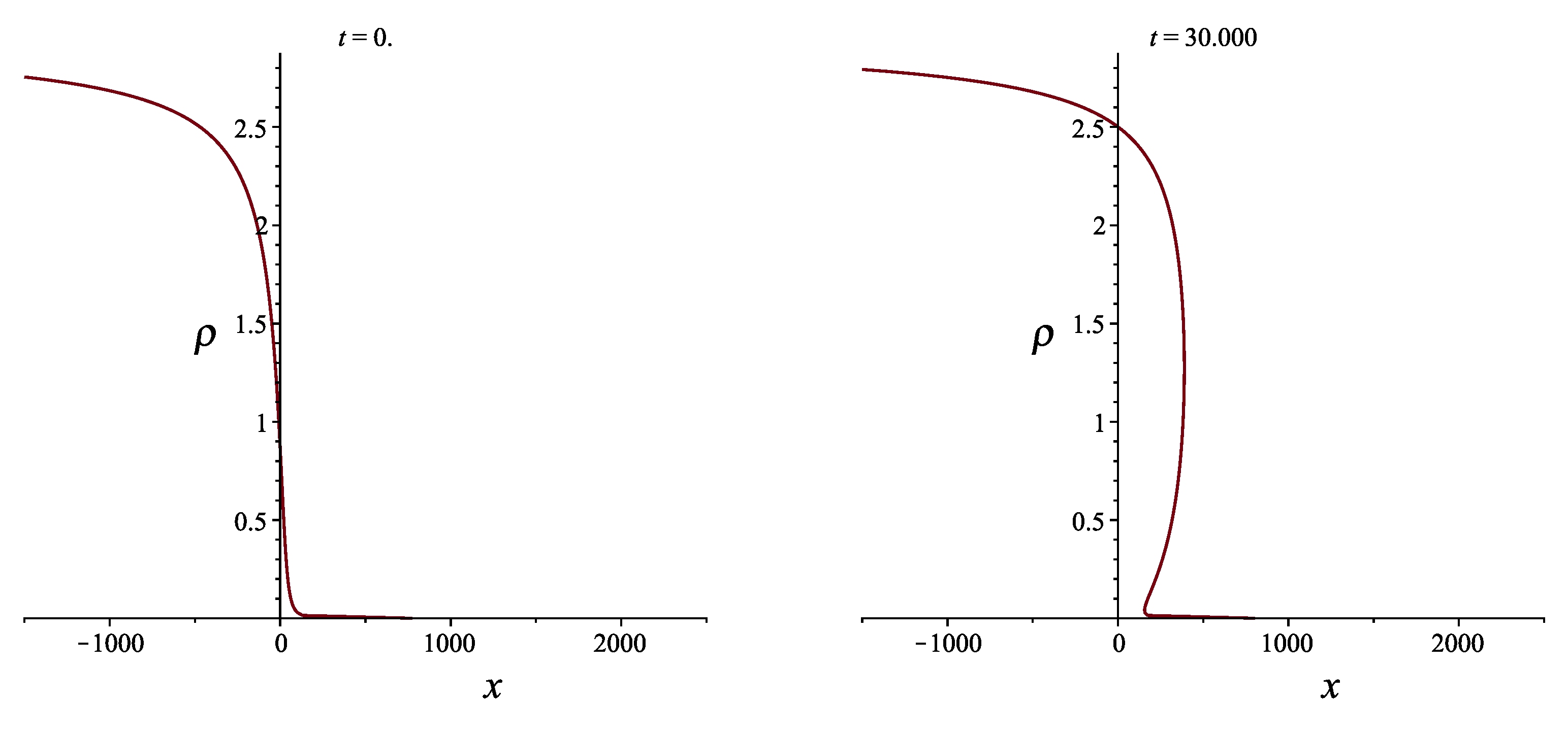
where we have already substituted $A\left(\rho \right)$ from (15), and ${\alpha }_2$, ${\alpha }_3$ are constants. The graph of a multivalued solution for the density is shown in Figure 2. We used substitution (16), where $C_5=240$, $n=3$, together with $C_2=1$, ${\alpha }_1=1$, ${\alpha }_2=2$, ${\alpha }_3=1$.

3.2. Caustics and Shockwaves

We can see that solution given by (23) and (24) is, in general, multivalued. To figure out where the two-dimensional manifold N given by (23) and (24) has singularities of projection to the plane of independent variables, one needs to find zeroes of the two-form $dt\wedge dx$. Condition ${(dt\wedge dx)|}_N=0$ gives us a curve in the plane ${\mathbb{R}}^2(t,x)$ called caustic. Choosing $\rho$ as a coordinate on the caustic, we get its equations in a parametric form:

$$\begin{array}{cc}\hfill x\left(\rho \right)& =-\frac{1}{2{\alpha }_1}\left(2C_{1}ln\rho +C_1(C_3^3{\rho }^3-4{\rho }^2{C}_3^2+3C_3\rho -2)+C_3{C}_2^3+2{\alpha }_1{\alpha }_3\right)\pm \hfill \\ & \pm \frac{C_2{(C_3\rho -1)}^2}{{\alpha }_1{\rho }^2}\sqrt{C_1{\rho }^3+C_5{\left(C_3+\frac{C_7}{\rho }\right)}^{C_6}}-\frac{C_5{\left(C_3+\frac{C_7}{\rho }\right)}^{C_6}}{2(C_6+2)(C_6+3)C_7^3{\alpha }_1(C_6+1){\rho }^3}·\hfill \\ & ·\left(C_3^3(-4+C_7^3(C_6^3+6C_6^2+11C_6+6)+(-2C_6-6)C_7){\rho }^3\right.-\hfill \\ & -2C_7(\left(2(C_6^3+6C_6^2+11C_6+6)\right)C_7^2+(-C_6^2-3C_6)C_7-C_6)C_3^2{\rho }^2+\hfill \\ & +\left.C_7^2(C_6+1)((C_6+3)(5C_6+12)C_7-2C_6)C_3\rho -2C_7^3(C_6+4)(C_6+2)(C_6+1)\right),\hfill \end{array}$$

(25)

$$t\left(\rho \right)=-{\alpha }_2-\frac{C_2{C}_3}{{\alpha }_1}\pm \frac{{(C_3\rho -1)}^2}{{\alpha }_1{\rho }^2}\sqrt{C_1{\rho }^3+C_5{\left(C_3+\frac{C_7}{\rho }\right)}^{C_6}}.$$

(26)

To construct a discontinuous solution from the multivalued one given by (23) and (24), we use the mass conservation law. Equation (11) with the velocity u found from (23) in terms of t and $\rho$ takes the form:

$${\rho }_t+{\left(\rho \frac{{\alpha }_1\rho (t+{\alpha }_2)+C_2}{1-C_3\rho }\right)}_x=0,$$

and therefore the conservation law is

$$\Theta =\rho dx-\rho \frac{{\alpha }_1\rho (t+{\alpha }_2)+C_2}{1-C_3\rho }dt.$$

Its restriction ${\Theta |}_N$ to the manifold N given by (23) and (24) is a closed form, locally ${\Theta |}_N=dH$, and the potential $H(\rho ,t)$ equals

$$\begin{array}{cc}\hfill H(\rho ,t)& =\frac{\rho }{2{\alpha }_1{(C_3\rho -1)}^2}\left(C_1{C}_3^3{\rho }^3-4C_1{C}_3^2{\rho }^2+\rho \left(C_2^2{C}_3^2+(2C_2(t+{\alpha }_2){\alpha }_1+5C_1)C_3+{\alpha }_1^2{(t+{\alpha }_2)}^2\right)-2C_1\right)-\hfill \\ & -\frac{C_5{\left(C_3+\frac{C_7}{\rho }\right)}^{C_6}}{(C_6+2){\alpha }_1{C}_7^2(C_6+1){\rho }^2}(C_3\rho +C_7)(C_3(1+(C_6+2)C_7)\rho -(C_6+1)C_7).\hfill \end{array}$$

The discontinuity line, or a shockwave front, is found from the system of equations

$$H({\rho }_1,t)=H({\rho }_2,t),x({\rho }_1,t)=x({\rho }_2,t),$$

where $x(\rho ,t)$ is obtained from (23) and (24) by eliminating u. Caustics along with the shockwave front are shown in Figure 3. Note that the picture is similar to that in the case of phase transitions.

The final result here is the expression for the time interval, within which the solution (23) and (24) is smooth.

Theorem 4.

The solution given by (23) and (24) is smooth and unique in the time interval $t\in [0,t^{*})$, where

$$t^{*}=\frac{1}{{\alpha }_1}\left(-C_2{C}_3-{\alpha }_1{\alpha }_2+{(C_3-3)}^2\sqrt{\frac{C_1}{27}+C_5{(C_3+3C_7)}^{C_6}}\right),$$

and in the case of (16), where $C_5=240$, $n=3$, together with $C_2=1$, ${\alpha }_1=1$, ${\alpha }_2=2$, ${\alpha }_3=1$ approximately $t^{*}=12.53$.

3.3. Phase Transitions

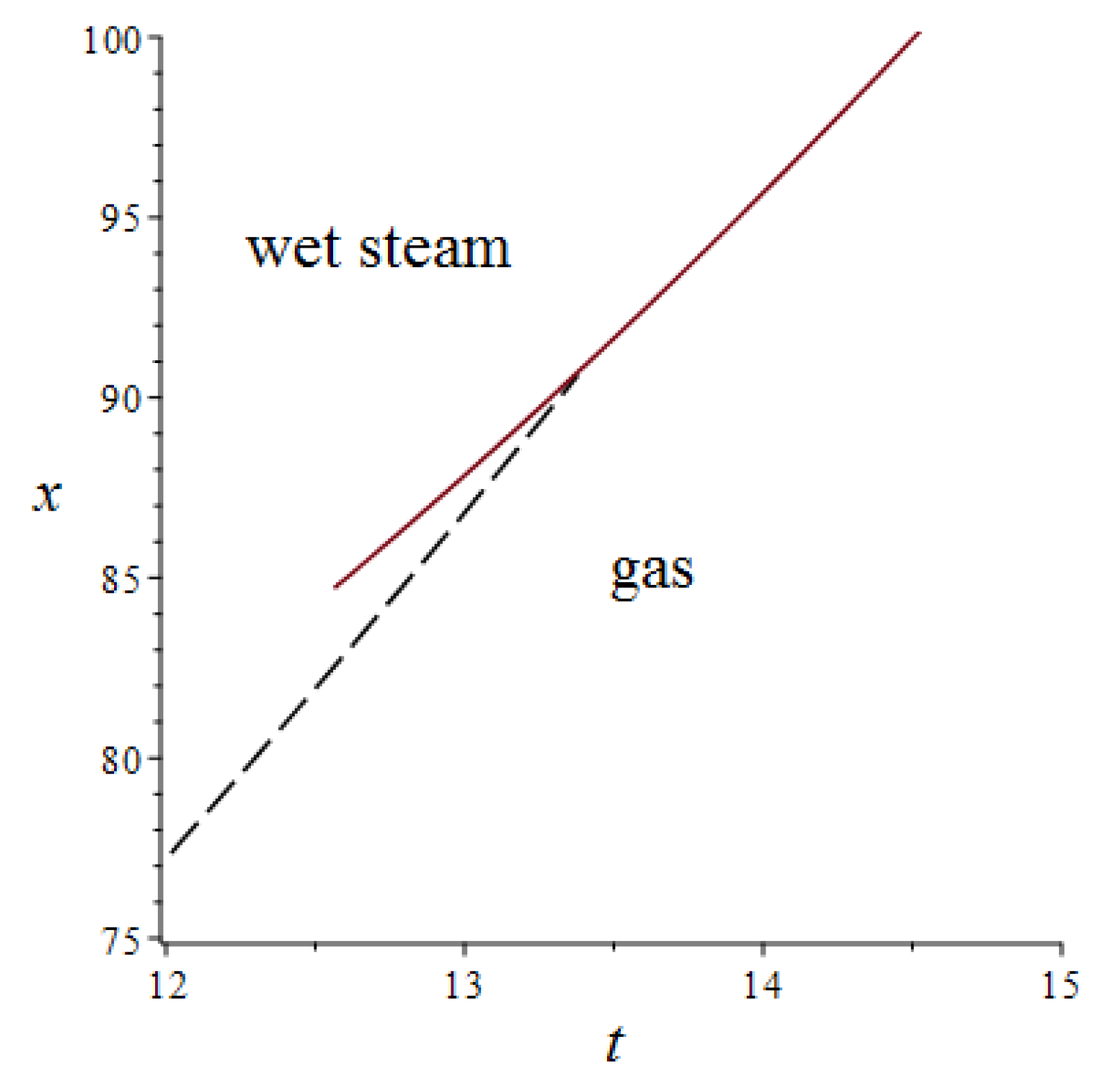
Having a solution, one can remove the phase transition curve from the space of thermodynamic variables to ${\mathbb{R}}^2(t,x)$. Indeed, on the one hand, we have all the thermodynamic parameters as functions of $(t,x)$. On the other hand, we have conditions on phase transitions (7) in the space of thermodynamic variables. In combination, they give us a curve of phase transitions in $(t,x)$ plane. Phase transitions together with the shockwave are presented in Figure 4. We use substitution (16), where $C_5=240$, $n=3$, together with $C_2=1$, ${\alpha }_1=1$, ${\alpha }_2=2$, ${\alpha }_3=1$.

4. Discussion

In the present work, we analyze critical phenomena in gas flows of purely thermodynamic nature, which are phase transitions and shockwaves arising from singularities of solutions to the Euler system. To obtain such solutions, we use a differential constraint compatible with the original system. In this work, it is found in a purely computational way, and how to get it in a more constructive way seems interesting. One possible way to find such constraints is using differential invariants. Then, constraints can be found constructively by solving quotient PDEs (see [32] for details), which was successfully realized by Schneider [22]. We hope to make use of this method in future research. The analysis of phase transitions shows that sometimes shockwaves can be accompanied with phase transitions, which is shown in Figure 4, since the phase transition curve intersects the shockwave front, and on the one side of the discontinuity curve we observe a pure gas phase, while on the other side we can see a wet steam.

References

- Arnold, V. Singularities of Caustics and Wave Fronts; Springer: Dordrecht, The Netherlands, 1990. [Google Scholar]
- Arnold, V. Catastrophe Theory; Springer: Berlin/Heidelberg, Germany, 1984. [Google Scholar]
- Arnold, V.; Gusein-Zade, S.; Varchenko, A. Singularities of Differentiable Maps; Birkhäuser: Basel, Switzerland, 1985. [Google Scholar]
- Zeldovich, A.; Kompaneets, I. Theory of Detonation; Academic Press: Cambridge, MA, USA, 1960. [Google Scholar]
- Huang, S.J.; Wang, R. On blowup phenomena of solutions to the Euler equations for Chaplygin gases. Appl. Math. Comput. 2013, 219, 4365–4370. [Google Scholar] [CrossRef]
- Rosales, R.; Tabak, E. Caustics of weak shock waves. Phys. Fluids 1997, 10, 206–222. [Google Scholar] [CrossRef] [Green Version]
- Chaturvedi, R.; Gupta, P.; Singh, L.P. Evolution of weak shock wave in two-dimensional steady supersonic flow in dusty gas. Acta Astronaut. 2019, 160, 552–557. [Google Scholar] [CrossRef]
- Poludnenko, A.; Oran, E. The interaction of high-speed turbulence with flames: Global properties and internal flame structure. Combust. Flame 2010, 157, 995–1011. [Google Scholar] [CrossRef] [Green Version]
- Poludnenko, A.; Gardiner, T.; Oran, E. Spontaneous Transition of Turbulent Flames to Detonations in Unconfined Media. Phys. Rev. Lett. 2011, 107, 054501. [Google Scholar] [CrossRef] [PubMed]
- Lychagin, V.; Roop, M. Shock waves in Euler flows of gases. Lobachevskii J. Math. 2020, 41, 2466–2472. [Google Scholar]
- Kushner, A.; Lychagin, V.; Rubtsov, V. Contact Geometry and Nonlinear Differential Equations; Cambridge University Press: Cambridge, UK, 2007. [Google Scholar]
- Vinogradov, A.; Krasilshchik, I. (Eds.) Symmetries and Conservation Laws for Differential Equations of Mathematical Physics; Factorial: Moscow, Russia, 1997. [Google Scholar]
- Vinogradov, A.; Krasilshchik, I.; Lychagin, V. Geometry of Jet Spaces and Nonlinear Partial Differential Equations; Gordon and Breach: New York, NY, USA, 1996. [Google Scholar]
- Ovsiannikov, L. Group Analysis of Differential Equations; Academic Press: Cambridge, MA, USA, 1982. [Google Scholar]
- Olver, P. Applications of Lie Groups to Differential Equations; Springer: New York, NY, USA, 1986. [Google Scholar]
- Tunitsky, D. On multivalued solutions of equations of one-dimensional gas flow. In Proceedings of the 12th International Conference “Management of Large-Scale System Development” (MLSD), Moscow, Russia, 1–3 October 2019. [Google Scholar]
- Lychagin, V. Singularities of multivalued solutions of nonlinear differential equations, and nonlinear phenomena. Acta Appl. Math. 1985, 3, 135–173. [Google Scholar] [CrossRef]
- Akhmetzyanov, A.; Kushner, A.; Lychagin, V. Control of displacement front in a model of immiscible two-phase flow in porous media. Dokl. Math. 2016, 94, 378–381. [Google Scholar] [CrossRef]
- Akhmetzyanov, A.; Kushner, A.; Lychagin, V. Integrability of Buckley-Leverett’s filtration model. IFAC PapersOnLine 2016, 49, 1251–1254. [Google Scholar]
- Akhmetzyanov, A.; Kushner, A.; Lychagin, V. Shock waves in initial boundary value problem for filtration in two-phase 2-dimensional porous media. Glob. Stoch. Anal. 2016, 3, 41–46. [Google Scholar]
- Kruglikov, B.; Lychagin, V. Compatibility, Multi-Brackets and Integrability of Systems of PDEs. Acta Appl. Math. 2010, 109, 151–196. [Google Scholar] [CrossRef] [Green Version]
- Schneider, E. Solutions of second-order PDEs with first-order quotients. arXiv 2020, arXiv:2005.06794. [Google Scholar]
- Lychagin, V.; Yumaguzhin, V. On Geometric Structures of 2-Dimensional Gas Dynamics Equations. Lobachevskii J. Math. 2009, 30, 327–332. [Google Scholar] [CrossRef]
- Lychagin, V.; Yumaguzhin, V. Minkowski Metrics on Solutions of the Khokhlov-Zabolotskaya Equation. Lobachevskii J. Math. 2009, 30, 333–336. [Google Scholar] [CrossRef]
- Anderson, I.; Torre, C.G. The Differential Geometry Package. Downloads. 2016, Paper 4. Available online: http://digitalcommons.usu.edu/dg_downloads/4 (accessed on 27 November 2020).
- Gibbs, J.W. A Method of Geometrical Representation of the Thermodynamic Properties of Substances by Means of Surfaces. Trans. Conn. Acad. 1873, 1, 382–404. [Google Scholar]
- Mrugala, R. Geometrical formulation of equilibrium phenomenological thermodynamics. Rep. Math. Phys. 1978, 14, 419–427. [Google Scholar] [CrossRef]
- Ruppeiner, G. Riemannian geometry in thermodynamic fluctuation theory. Rev. Mod. Phys. 1995, 67, 605–659. [Google Scholar] [CrossRef]
- Lychagin, V. Contact Geometry, Measurement, and Thermodynamics. In Nonlinear PDEs, Their Geometry and Applications; Kycia, R., Schneider, E., Ulan, M., Eds.; Birkhäuser: Cham, Switzerland, 2019; pp. 3–52. [Google Scholar]
- Lychagin, V.; Roop, M. Critical phenomena in filtration processes of real gases. Lobachevskii J. Math. 2020, 41, 382–399. [Google Scholar] [CrossRef]
- Kushner, A.; Lychagin, V.; Roop, M. Optimal Thermodynamic Processes for Gases. Entropy 2020, 22, 448. [Google Scholar] [CrossRef] [PubMed]
- Kruglikov, B.; Lychagin, V. Global Lie-Tresse theorem. Selecta Math. 2016, 22, 1357–1411. [Google Scholar] [CrossRef] [Green Version]
Figure 1.
Singularities of the van der Waals Legendrian manifold: caustic (black line) and phase transition curve (red line) in coordinates (a); and the curve of phase transition in (b). Points of the phase transition curve with the same values of pressure p and temperature T and different values of density correspond to the liquid phase and the gas phase, respectively, while points between and correspond to wet steam.
Figure 2.
Graph of the density in case of for time moments , .
Figure 3.
Caustic (black) and shockwave front (red) for .
Figure 4.
Phase transition curve (dash line) and shockwave front (red line).
Publisher’s Note: MDPI stays neutral with regard to jurisdictional claims in published maps and institutional affiliations. |
© 2020 by the authors. Licensee MDPI, Basel, Switzerland. This article is an open access article distributed under the terms and conditions of the Creative Commons Attribution (CC BY) license (http://creativecommons.org/licenses/by/4.0/).
Share and Cite
MDPI and ACS Style
Lychagin, V.; Roop, M. Singularities in Euler Flows: Multivalued Solutions, Shockwaves, and Phase Transitions. Symmetry 2021, 13, 54. https://0-doi-org.brum.beds.ac.uk/10.3390/sym13010054
AMA Style
Lychagin V, Roop M. Singularities in Euler Flows: Multivalued Solutions, Shockwaves, and Phase Transitions. Symmetry. 2021; 13(1):54. https://0-doi-org.brum.beds.ac.uk/10.3390/sym13010054
Chicago/Turabian StyleLychagin, Valentin, and Mikhail Roop. 2021. "Singularities in Euler Flows: Multivalued Solutions, Shockwaves, and Phase Transitions" Symmetry 13, no. 1: 54. https://0-doi-org.brum.beds.ac.uk/10.3390/sym13010054
Note that from the first issue of 2016, this journal uses article numbers instead of page numbers. See further details here.