Influence of Time Delay on Controlling the Non-Linear Oscillations of a Rotating Blade

Abstract

Time delay is an obstacle in the way of actively controlling non-linear vibrations. In this paper, a rotating blade’s non-linear oscillations are reduced via a time-delayed non-linear saturation controller (NSC). This controller is excited by a positive displacement signal measured from the sensors on the blade, and its output is the suitable control force applied onto the actuators on the blade driving it to the desired minimum vibratory level. Based on the saturation phenomenon, the blade vibrations can be saturated at a specific level while the rest of the energy is transferred to the controller. This can be done by adjusting the controller natural frequency to be one half of the blade natural frequency. The whole behavior is governed by a system of first-order differential equations gained by the method of multiple scales. Different responses are included to show the influences of time delay on the closed-loop control process. Also, a good agreement can be noticed between the analytical curves and the numerically simulated ones.

1. Introduction

The rotating blade is considered the cornerstone of the turbo-machinery industry. Due to its high spinning speed and distributed mass, it may suffer from unwanted vibrations. A huge number of researchers have focused their attention on analyzing and/or controlling (passively or actively) such vibrations for safe operation. Active control techniques have proved their flexibility and adaptation to the control process than passive control techniques that were used as a back-up for active control. However, active control techniques have inherently exhibited a huge issue of time delay. This issue arose because of the delay in acquiring the feedback signal and/or applying the control signal. Yao et al. [1] worked on a thin-walled rotating blade and considered a preliminary twisting, a preliminary setting for this blade. They also examined the whole behavior in case of rotating speed variation. They utilized the Hamilton principle for extracting the blade’s equations of motion. Wang and Zhang [2] discussed a spinning blade stability where it had periodic time-varying coefficients for both the linear and non-linear geometric models. Yao et al. [3] investigated the air velocity variation which caused uncertainties in the aerodynamic load, the geometric non-linearity, the perturbed angular speed, and the centrifugal force. Sina and Haddadpour [4] examined both the axial and torsional vibrations of a thin-walled rotating box beam with preliminary twisting and primary-secondary warping. Wang and Qu [5] focused on the torsional excitation affecting a rotating beam which involved both quadratic and cubic non-linearities. Pesek et al. [6] achieved experimental and numerical works on a rotating blade’s interaction utilizing a frictional element that was placed in the shroud between the blade heads. Hamed and Amer [7] presented a non-linear saturation controller (NSC) study to suppress a non-linear structural composite beam’s vibration amplitude at the simultaneous resonance of sub-harmonic and internal cases. Bian et al. [8] examined the effects of the simultaneous resonance (primary resonance and $2:1$ internal resonance) on the chaotic dynamics and global bifurcations of a thin-walled compressor blade. Kim and Chung [9] introduced an accurate non-linear model of a rotating beam with elastic deformations for an efficient dynamic analysis. Li et al. [10] proposed an accurate analytical technique for studying the forced Mathieu oscillator based on the parameters variation method. Luo et al. [11] considered the centrifugal stress to investigate the accurate design prototype’s dynamic characteristics of a thin-walled rotating plate. Zhang et al. [12] utilized analytical and numerical techniques to study the local bifurcation and stability of a rotating blade accompanied by extremely hot supersonic gas flow. Zhao et al. [13] considered the thermal shock and tip-rub in a rotating plate to obtain its dynamic characteristics. Asghari and Hashemi [14] utilized the modified couple stress theory to consider the small-scale effects for analyzing the micro-spinning Rayleigh beams 3D vibrations. Cao et al. [15] investigated an aero-engine turbine blade’s vibrational behavior with preliminary twisting, preliminary setting angle, and thermal barrier coating layers. Kandil and Eissa [16] suppressed the two peaks of the positive position feedback (PPF) controller’s performance with imposed V-curves by coupling two additional non-linear saturation controllers (NSC) to the rotating blade. Farsadi et al. [17] modeled structurally thin-walled beams to study the aeroelastic behavior of the preliminary twisting and the high aspect ratio wings. Kandil and El-Gohary [18,19] studied the effects of time delay on the vibration control performance for reducing the oscillations of a rotating beam via proportional derivative (PD) and NSC controllers. Khaniki [20] concluded the disability of the nonlocal elastic theory differential form for presenting a reliable investigation on transverse vibrational behavior of rotating beams. Li et al. [21] built their dynamic model based on the finite element method in order to analyze the non-linear characteristics of a flexible blade contained in a centrifugal force field. Yao et al. [22] investigated the varying-rotating-speed blade dynamic responses to the supersonic airflow and the cross-section warping effect. Gu et al. [23] used the shallow shell theory considering the torsion and neglecting two radii of curvatures for treating the rotating blade as a cantilever pre-twisted panel with initial exponential function. The authors [24,25] presented the functionally graded rotating composite Timoshenko beams that were reinforced by carbon nanotubes or graphene platelets for studying their linear and non-linear free vibrations. Umer and Botto [26] studied experimentally the non-linear contact forces effect on the vibration amplitude of a rotating blade. Yang et al. [27] investigated the presence of $1:2$ internal resonance, primary parametric resonance, and $1/2$ subharmonic resonance to explore the non-linear vibrations of a carbon fiber-reinforced polymer laminated cylindrical shell. Yao et al. [28] considered a preliminary setting angle in building the model of a rotating cylindrical shell to investigate the aero-engine compressor blade non-linear dynamic responses. Zhang et al. [29] revealed the simultaneous resonance (both primary and internal $2:1$) of a rotating preliminary twisting blade which was subjected to a flap-wise gas excitation with thermal gradient. Khosravi et al. [30] presented the rotating composite beams that were reinforced by carbon nanotubes for studying the influence of uniform temperature elevation leading to instability. Han et al. [31] formulated the steady-state dynamic responses of rotating bending-torsion coupled composite Timoshenko beams subjected to distributive and/or concentrated harmonic loadings. Hamed et al. [32,33] applied either time-delayed PPF or PD controllers on a multi-excitation atomic force microscopy (AFM) model in order to extract the time delay effects on the vibration control process. It is worth mentioning the importance of the homotopy perturbation method (HPM) in solving linear and non-linear problems. He [34,35,36] proposed a new perturbation technique coupled with the homotopy technique where the equation’s small parameters were not required leading to eliminating the limitations of the traditional techniques. Noeiaghdam et al. [37] proposed the HPM to study the second-kind linear Volterra integral equations with a discontinuous kernel. They validated the solution’s accuracy by analyzing the convergence and error of the studied formulation. Hussain et al. [38] used the HPM to find an approximate analytical solution of the bi-stable Allen–Cahn equation. They observed a good agreement between the analytical and numerical solutions when recording the error estimates. Javeed et al. [39] presented the HPM for solving fractional-derivative partial differential equations, even though the ordinary-derivative partial differential equations were not defined in the given domain.

This work focuses on actively controlling a rotating blade’s non-linear oscillation via macro fiber composite (MFC) and non-linear saturation control algorithm. According to the active control process shown in Figure 1, the closed-loop control may suffer from time delay in acquiring the feedback signal (from MFC sensors) and/or applying the control signal (into MFC actuators). The wafers of sensors and actuators are implanted in the centroids of the bottom and top of the rotating blade, respectively. They are distributed along the blade’s length as shown in Figure 1. Based on the saturation controller, the blade vibrations can be saturated at a specific level while the rest of the energy is transferred to the controller. This can be done by adjusting the controller frequency ${\mathsf{\omega }}_{\mathrm{c}}$ to be one half of the blade frequency $\mathsf{\omega }$. In this work, all we care about in the measurement process is the time delay and its effect on the control process. The measurement noise was not considered in this model in order to focus our discussion on the time delay effect. We are including this issue in future work to make our controller more realistic. The whole behavior is governed by a system of first-order differential equations gained by the method of multiple scales. The stability criteria can be extracted due to Lyapunov’s linearization technique to indicate the time delay borders at which the whole system switches its stability.

2. The Amplitudes and Phases Equations of the Blade and Controller

This model derivation is given briefly in the Appendix A. As seen in Figure 1, the horizontal and vertical deflections of the blade’s cross-section have been represented by $x\left(t\right)$ and $y\left(t\right)$, respectively. This cross-section, subjected to harmonic excitation, is governed by the following equations of motion [1]:

$$\ddot{x}+2\mu \dot{x}+{\omega }^{2}x+{\alpha }_1\dot{y}+{\alpha }_{21}y+{\alpha }_3\left[x^3+x{y}^2\right]-{\alpha }_{41}x\left[2f_{0}f\cos \left(\mathsf{\Omega }t\right)+f^2{\cos }^2\left(\mathsf{\Omega }t\right)\right]=f{\alpha }_5\mathsf{\Omega }\sin \left(\mathsf{\Omega }t\right)$$

(1a)

$$\ddot{y}+2\mu \dot{y}+{\omega }^{2}y+{\alpha }_1\dot{x}+{\alpha }_{22}x+{\alpha }_3\left[y^3+x^{2}y\right]-{\alpha }_{42}y\left(2f_{0}f\cos \left(\mathsf{\Omega }t\right)+f^2{\cos }^2\left(\mathsf{\Omega }t\right)\right)=0,$$

(1b)

where $\mu$ is the viscous damping, $\omega$ is the natural frequency, {${\alpha }_1$, ${\alpha }_{21}$, ${\alpha }_{22}$} are the linear coupling parameters, ${\alpha }_3$ is the non-linear coupling parameter, {${\alpha }_{41}$, ${\alpha }_{42}$} are the parametric excitation coefficients, ${\alpha }_5$ is the external excitation coefficient, {$f_0$, $f$} are the excitation force amplitudes, and $\mathsf{\Omega }$ is the rotating blade’s angular speed. Applying the time-delayed saturation controller signal $u\left(t\right)$ to Equation (1), the overall equations will be:

$$\ddot{x}+2\mu \dot{x}+{\omega }^{2}x+{\alpha }_1\dot{y}+{\alpha }_{21}y+{\alpha }_3\left[x^3+x{y}^2\right]-{\alpha }_{41}x\left[2f_{0}f\cos \left(\mathsf{\Omega }t\right)+f^2{\cos }^2\left(\mathsf{\Omega }t\right)\right]=f{\alpha }_5\mathsf{\Omega }\sin \left(\mathsf{\Omega }t\right)+c_1{u}_{{\tau }_2}^2$$

(2a)

$$\ddot{y}+2\mu \dot{y}+{\omega }^{2}y+{\alpha }_1\dot{x}+{\alpha }_{22}x+{\alpha }_3\left[y^3+x^{2}y\right]-{\alpha }_{42}y\left(2f_{0}f\cos \left(\mathsf{\Omega }t\right)+f^2{\cos }^2\left(\mathsf{\Omega }t\right)\right)=0$$

(2b)

$$\ddot{u}+2{\mu }_c\dot{u}+{\omega }_c^{2}u=c_2{x}_{{\tau }_1}u,$$

(2c)

where ${\mu }_c$ is the controller’s damping, ${\omega }_c$ is its natural frequency, {$c_1$, $c_2$} are gains of the control and feedback signals, {${\tau }_1$, ${\tau }_2$} are delay times, $x_{{\tau }_1}=x\left(t-{\tau }_1\right)$ is the time-delayed feedback signal, and $u_{{\tau }_2}=u\left(t-{\tau }_2\right)$ is the time-delayed control signal. We can scale some parameters in Equation (2) to make them appear later in the perturbation equations by assuming the following:

$${\alpha }_1=\epsilon {\widehat{\alpha }}_1,{\alpha }_{21}=\epsilon {\widehat{\alpha }}_{21},{\alpha }_{22}=\epsilon {\widehat{\alpha }}_{22},{\alpha }_3=\epsilon {\widehat{\alpha }}_3,{\alpha }_{41}=\epsilon {\widehat{\alpha }}_{41},{\alpha }_{42}=\epsilon {\widehat{\alpha }}_{42},{\alpha }_5=\epsilon {\widehat{\alpha }}_5,c_{1, 2}=\epsilon {\widehat{c}}_{1, 2},\mu =\epsilon \widehat{\mu },{\mu }_c=\epsilon {\widehat{\mu }}_c,$$

(3)

where $\epsilon$ is an extremely small perturbation parameter. Hence, the multiple time scales ($T_0=t$ and $T_1=\epsilon t$) can be used to suppose approximate solutions of the following expansion forms [40]:

$$x\left(t;\epsilon \right)=x_0\left(T_0,T_1\right)+\epsilon x_1\left(T_0,T_1\right)+O\left({\epsilon }^2\right)$$

(4a)

$$y\left(t;\epsilon \right)=y_0\left(T_0,T_1\right)+\epsilon y_1\left(T_0,T_1\right)+O\left({\epsilon }^2\right)$$

(4b)

$$u\left(t;\epsilon \right)=u_0\left(T_0,T_1\right)+\epsilon u_1\left(T_0,T_1\right)+O\left({\epsilon }^2\right)$$

(4c)

$$x_{{\tau }_1}\left(t;\epsilon \right)=x_{0{\tau }_1}\left(T_0,T_1\right)+\epsilon x_{1{\tau }_1}\left(T_0,T_1\right)+O\left({\epsilon }^2\right)$$

(4d)

$$u_{{\tau }_2}\left(t;\epsilon \right)=u_{0{\tau }_2}\left(T_0,T_1\right)+\epsilon u_{1{\tau }_2}\left(T_0,T_1\right)+O\left({\epsilon }^2\right).$$

(4e)

Also, the first and second time derivatives in Equation (2) can be transformed into:

$$\frac{d}{dt}=\frac{\partial }{\partial T_0}+\epsilon \frac{\partial }{\partial T_1}+O\left({\epsilon }^2\right)=D_0+\epsilon D_1+O\left({\epsilon }^2\right)$$

(5a)

$$\frac{d^2}{d{t}^2}=\frac{{\partial }^2}{\partial T_0^2}+2\epsilon \frac{{\partial }^2}{\partial T_0\partial T_1}+O\left({\epsilon }^2\right)=D_0^2+2\epsilon D_0{D}_1+O\left({\epsilon }^2\right).$$

(5b)

Substituting Equations (3)–(5) into Equation (2) then comparing the powers of $\epsilon$ on both sides yield:

$$O\left({\epsilon }^0\right):\hspace{1em}\hspace{1em}\hspace{1em}\hspace{1em}\hspace{1em}\hspace{1em}\hspace{1em}\hspace{1em}\hspace{1em}\hspace{1em}\hspace{1em}\hspace{1em}\hspace{1em}\hspace{1em}\hspace{1em}\hspace{1em}$$

$$D_0^2{x}_0+{\omega }^2{x}_0=0$$

(6a)

$$D_0^2{y}_0+{\omega }^2{y}_0=0$$

(6b)

$$D_0^2{u}_0+{\omega }_c^2{u}_0=0$$

(6c)

$$O\left({\epsilon }^1\right):\hspace{1em}\hspace{1em}\hspace{1em}\hspace{1em}\hspace{1em}\hspace{1em}\hspace{1em}\hspace{1em}\hspace{1em}\hspace{1em}\hspace{1em}\hspace{1em}\hspace{1em}\hspace{1em}\hspace{1em}\hspace{1em}$$

$$\begin{gathered} D_0^2{x}_1+{\omega }^2{x}_1=-2D_1{D}_0{x}_0-2\widehat{\mu }{D}_0{x}_0-{\widehat{\alpha }}_1{D}_0{y}_0-{\widehat{\alpha }}_{21}{y}_0-{\widehat{\alpha }}_3\left[x_0^3+x_0{y}_0^2\right] \\ +{\widehat{\alpha }}_{41}{x}_0\left[f_{0}f\left(e^{i\mathsf{\Omega }{T}_0}+e^{-i\mathsf{\Omega }{T}_0}\right)+\frac{f^2}{4}{\left(e^{i\mathsf{\Omega }{T}_0}+e^{-i\mathsf{\Omega }{T}_0}\right)}^2\right]-i\frac{f{\widehat{\alpha }}_5\mathsf{\Omega }}{2}\left(e^{i\mathsf{\Omega }{T}_0}-e^{-i\mathsf{\Omega }{T}_0}\right)+{\widehat{c}}_1{u}_{0{\tau }_2}^2 \end{gathered}$$

(7a)

$$\begin{gathered} D_0^2{y}_1+{\omega }^2{y}_1=-2D_1{D}_0{y}_0-2\widehat{\mu }{D}_0{y}_0-{\widehat{\alpha }}_1{D}_0{x}_0-{\widehat{\alpha }}_{22}{x}_0-{\widehat{\alpha }}_3\left[y_0^3+x_0^2{y}_0\right] \\ +{\widehat{\alpha }}_{42}{y}_0\left[f_{0}f\left(e^{i\mathsf{\Omega }{T}_0}+e^{-i\mathsf{\Omega }{T}_0}\right)+\frac{f^2}{4}{\left(e^{i\mathsf{\Omega }{T}_0}+e^{-i\mathsf{\Omega }{T}_0}\right)}^2\right] \end{gathered}$$

(7b)

$$D_0^2{u}_1+{\omega }_c^2{u}_1=-2D_1{D}_0{u}_0-2{\widehat{\mu }}_c{D}_0{u}_0+{\widehat{c}}_2{x}_{0{\tau }_1}{u}_0.$$

(7c)

The complex form solutions of Equation (6) and the time-delayed signals can be expressed as follows:

$$x_0=A_1{e}^{i\omega T_0}+{\overline{A}}_1{e}^{-i\omega T_0}$$

(8a)

$$x_{0{\tau }_1}\cong A_1{e}^{i\omega \left(T_0-{\tau }_1\right)}+{\overline{A}}_1{e}^{-i\omega \left(T_0-{\tau }_1\right)}$$

(8b)

$$y_0=A_2{e}^{i\omega T_0}+{\overline{A}}_2{e}^{-i\omega T_0}$$

(8c)

$$u_0=A_3{e}^{i{\omega }_c{T}_0}+{\overline{A}}_3{e}^{-i{\omega }_c{T}_0}$$

(8d)

$$u_{0{\tau }_2}\cong A_3{e}^{i{\omega }_c\left(T_0-{\tau }_2\right)}+{\overline{A}}_3{e}^{-i{\omega }_c\left(T_0-{\tau }_2\right)},$$

(8e)

where the coefficients $A_1$ to $A_3$ and their complex conjugates (${\overline{A}}_1$ to ${\overline{A}}_3$) are functions of the slow time $T_1$. We have initially tested the simultaneous resonance case ($\mathsf{\Omega }=\omega =2{\omega }_c$) as the worst resonance case. This can be described by the parameters ${\sigma }_1$ and ${\sigma }_2$ to represent the differences in the proposed resonance case as $\mathsf{\Omega }=\omega +{\sigma }_1=\omega +\epsilon {\widehat{\sigma }}_1$ and $2{\omega }_c=\omega +{\sigma }_2=\omega +\epsilon {\widehat{\sigma }}_2$. They are used with Equation (8) into Equation (7) to get the solvability conditions:

$$\begin{gathered} -2i\omega {\dot{A}}_1-2i\mu \omega A_1-i\omega {\alpha }_1{A}_2-{\alpha }_{21}{A}_2-3{\alpha }_3{A}_1^2{\overline{A}}_1-{\alpha }_3{\overline{A}}_1{A}_2^2-2{\alpha }_3{A}_1{A}_2{\overline{A}}_2+\frac{{\alpha }_{41}{f}^2}{2}{A}_1+\frac{{\alpha }_{41}{f}^2}{4}{\overline{A}}_1{e}^{2i{\sigma }_{1}t} \\ -\frac{i}{2}{\alpha }_5\mathsf{\Omega }f{e}^{i{\sigma }_{1}t}+c_1{A}_3^2{e}^{i\left({\sigma }_{2}t-2{\omega }_{\mathrm{c}}{\tau }_2\right)}=0 \end{gathered}$$

(9a)

$$-2i\omega {\dot{A}}_2-2i\mu \omega A_2-i\omega {\alpha }_1{A}_1-{\alpha }_{22}{A}_1-3{\alpha }_3{A}_2^2{\overline{A}}_2-{\alpha }_3{A}_1^2{\overline{A}}_2-2{\alpha }_3{A}_1{\overline{A}}_1{A}_2+\frac{{\alpha }_{42}{f}^2}{2}{A}_2+\frac{{\alpha }_{42}{f}^2}{4}{\overline{A}}_2{e}^{2i{\sigma }_{1}t}=0$$

(9b)

$$-2i{\omega }_c{\dot{A}}_3-2i{\mu }_c{\omega }_c{A}_3+c_2{A}_1{\overline{A}}_3{e}^{-i\left({\sigma }_{2}t+\omega {\tau }_1\right)}=0.$$

(9c)

The quantities ${\mathrm{A}}_n$ ($n=1$, $2$, $3$) can be rewritten in the exponential form, including the amplitudes $a_n$ and phases ${\beta }_n$ as follows:

$$A_n=\frac{1}{2}{a}_n{e}^{i{\beta }_n}\Rightarrow {\dot{A}}_n=\frac{{\dot{a}}_n}{2}{e}^{i{\beta }_n}+i\frac{a_n}{2}{\dot{\beta }}_n{e}^{i{\beta }_n}.$$

(10)

An autonomous system of differential equations can be obtained by substituting Equation (10) into Equation (9) as:

$$\begin{gathered} {\dot{a}}_1=-\mu a_1-\frac{{\alpha }_1}{2}{a}_2\cos {\varphi }_2-\frac{{\alpha }_{21}}{2\omega }{a}_2\sin {\varphi }_2-\frac{{\alpha }_3}{8\omega }{a}_1{a}_2^2\sin \left(2{\varphi }_2\right)+\frac{{\alpha }_{41}{f}^2}{8\omega }{a}_1\sin \left(2{\varphi }_1\right)-\frac{{\alpha }_5\mathsf{\Omega }f}{2\omega }\cos {\varphi }_1 \\ +\frac{c_1}{4\omega }{a}_3^2\sin \left({\varphi }_3-2{\omega }_c{\tau }_2\right) \end{gathered}$$

(11a)

$$\begin{gathered} {\dot{\varphi }}_1={\sigma }_1+\frac{{\alpha }_1}{2}\frac{a_2}{a_1}\sin {\varphi }_2-\frac{{\alpha }_{21}}{2\omega }\frac{a_2}{a_1}\cos {\varphi }_2-\frac{{\alpha }_3}{4\omega }{a}_2^2-\frac{{\alpha }_3}{8\omega }{a}_2^2\cos \left(2{\varphi }_2\right)-\frac{3{\alpha }_3}{8\omega }{a}_1^2+\frac{{\alpha }_{41}{f}^2}{8\omega }\cos \left(2{\varphi }_1\right)+\frac{{\alpha }_{41}{f}^2}{4\omega } \\ +\frac{{\alpha }_5\mathsf{\Omega }f}{2\omega }\frac{\sin {\varphi }_1}{a_1}+\frac{c_1}{4\omega }\frac{a_3^2}{a_1}\cos \left({\varphi }_3-2{\omega }_c{\tau }_2\right) \end{gathered}$$

(11b)

$${\dot{a}}_2=-\mu a_2-\frac{{\alpha }_1}{2}{a}_1\cos {\varphi }_2+\frac{{\alpha }_{22}}{2\omega }{a}_1\sin {\varphi }_2+\frac{{\alpha }_3}{8\omega }{a}_1^2{a}_2\sin \left(2{\varphi }_2\right)+\frac{{\alpha }_{42}{f}^2}{8\omega }{a}_2\sin \left(2{\varphi }_1-2{\varphi }_2\right)$$

(11c)

$$\begin{gathered} {\dot{\varphi }}_2=\frac{{\alpha }_1}{2}\frac{a_1}{a_2}\sin {\varphi }_2+\frac{{\alpha }_{22}}{2\omega }\frac{a_1}{a_2}\cos {\varphi }_2+\frac{{\alpha }_3}{4\omega }{a}_1^2+\frac{{\alpha }_3}{8\omega }{a}_1^2\cos \left(2{\varphi }_2\right)+\frac{3{\alpha }_3}{8\omega }{a}_2^2-\frac{{\alpha }_{42}{f}^2}{8\omega }\cos \left(2{\varphi }_1-2{\varphi }_2\right)-\frac{{\alpha }_{42}{f}^2}{4\omega } \\ +\frac{{\alpha }_1}{2}\frac{a_2}{a_1}\sin {\varphi }_2-\frac{{\alpha }_{21}}{2\omega }\frac{a_2}{a_1}\cos {\varphi }_2-\frac{{\alpha }_3}{4\omega }{a}_2^2-\frac{{\alpha }_3}{8\omega }{a}_2^2\cos \left(2{\varphi }_2\right)-\frac{3{\alpha }_3}{8\omega }{a}_1^2+\frac{{\alpha }_{41}{f}^2}{8\omega }\cos \left(2{\varphi }_1\right)+\frac{{\alpha }_{41}{f}^2}{4\omega } \\ +\frac{{\alpha }_5\mathsf{\Omega }f}{2\omega }\frac{\sin {\varphi }_1}{a_1}+\frac{c_1}{4\omega }\frac{a_3^2}{a_1}\cos \left({\varphi }_3-2{\omega }_c{\tau }_2\right) \end{gathered}$$

(11d)

$${\dot{a}}_3=-{\mu }_c{a}_3-\frac{c_2}{4{\omega }_c}{a}_1{a}_3\sin \left({\varphi }_3+\omega {\tau }_1\right)$$

(11e)

$$\begin{gathered} {\dot{\varphi }}_3={\sigma }_2-\frac{c_2}{2{\omega }_c}{a}_1\cos \left({\varphi }_3+\omega {\tau }_1\right)+\frac{{\alpha }_1}{2}\frac{a_2}{a_1}\sin {\varphi }_2-\frac{{\alpha }_{21}}{2\omega }\frac{a_2}{a_1}\cos {\varphi }_2-\frac{{\alpha }_3}{4\omega }{a}_2^2-\frac{{\alpha }_3}{8\omega }{a}_2^2\cos \left(2{\varphi }_2\right)-\frac{3{\alpha }_3}{8\omega }{a}_1^2+\frac{{\alpha }_{41}{f}^2}{4\omega } \\ +\frac{{\alpha }_{41}{f}^2}{8\omega }\cos \left(2{\varphi }_1\right)+\frac{{\alpha }_5\mathsf{\Omega }f}{2\omega }\frac{\sin {\varphi }_1}{a_1}+\frac{c_1}{4\omega }\frac{a_3^2}{a_1}\cos \left({\varphi }_3-2{\omega }_c{\tau }_2\right), \end{gathered}$$

(11f)

where ${\varphi }_1={\sigma }_{1}t-{\beta }_1$, ${\varphi }_2={\beta }_2-{\beta }_1$, and ${\varphi }_3={\sigma }_{2}t+2{\beta }_3-{\beta }_1$. The steady-state analysis of the studied blade model can be fulfilled by imposing the conditions ${\dot{a}}_n={\dot{\varphi }}_n=0$ into Equation (11). The resulting non-linear algebraic equations system cannot be solved analytically, leading us to adopt the Newton–Raphson numerical technique. The extracted equilibrium solutions of the amplitudes $a_n$ and phases ${\varphi }_n$ can be classified as either stable or unstable, according to Lyapunov’s linearization technique [7,16,18,19,32,33,40].

3. Results and Discussion

3.1. Relation between the Parameters and the Steady-State Amplitudes

This subsection involves the steady-state response curves of the blade vibrational amplitudes versus different parameters. These curves are plotted depending on the fixed points of Equation (11). In the following figures, the solid lines refer to stable trajectories, while the dashed lines refer to unstable ones. The asterisks refer to bifurcation points where SN is the Saddle-Node point, H is Hopf point, and PF is the pitchfork point. Regarding the whole system safe operation, the adopted parameter’s values are: $\mu =0.5$, ${\mu }_c=0.001$, $\mathsf{\Omega }=\omega =2{\omega }_c=100$, ${\alpha }_1=-0.82$, ${\alpha }_{21}=-0.003$, ${\alpha }_{22}=-0.001$, ${\alpha }_3=0.9$, ${\alpha }_{41}=0.55$, ${\alpha }_{42}=0.5$, ${\alpha }_5=6.55$, $f_0=7$, $f=2$, $c_1=5$, $c_2=15$, ${\sigma }_1={\sigma }_2=0$, ${\tau }_1={\tau }_2=0$. Figure 2 shows the effect of the feedback signal delay ${\tau }_1$ on the blade and controller vibrational amplitudes at no control signal delay (${\tau }_2=0$). The amplitudes switch from stability to instability at ${\tau }_1\cong 0.0039,$ which is considered a border value of the stable amplitudes region. Figure 3 clarifies the effect of ${\tau }_2$ on the blade and controller vibrational amplitudes at ${\tau }_1=0$. It is the same as in Figure 2 where ${\tau }_2\cong 0.0039$ is considered a border value of the stable amplitudes region. This guides us to conclude a border line equation of the stable amplitudes region based on Figure 2 and Figure 3 to be ${\tau }_1+{\tau }_2=0.0039$. As a result, the constraint ${\tau }_1+{\tau }_2<0.0039$ is guaranteeing stable amplitudes, as shown in the shaded region of Figure 4.

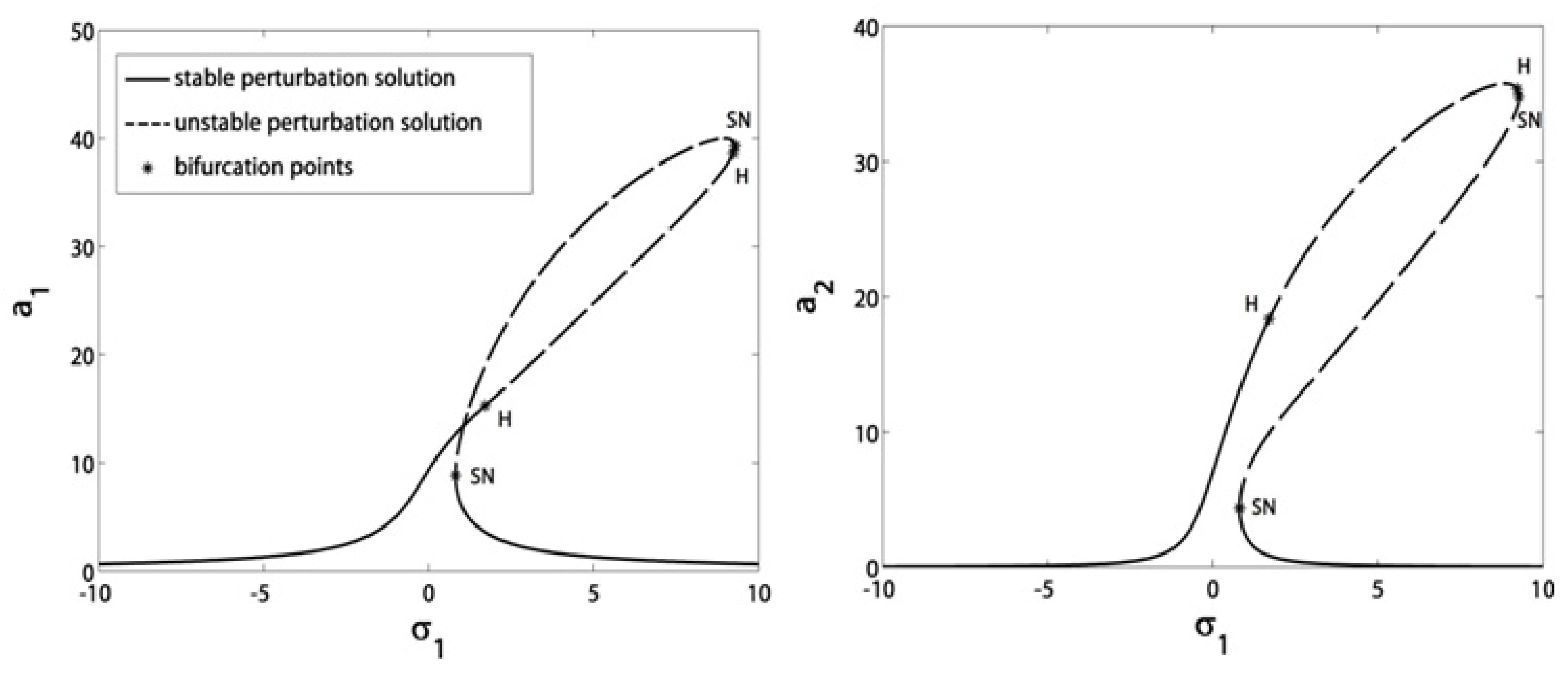
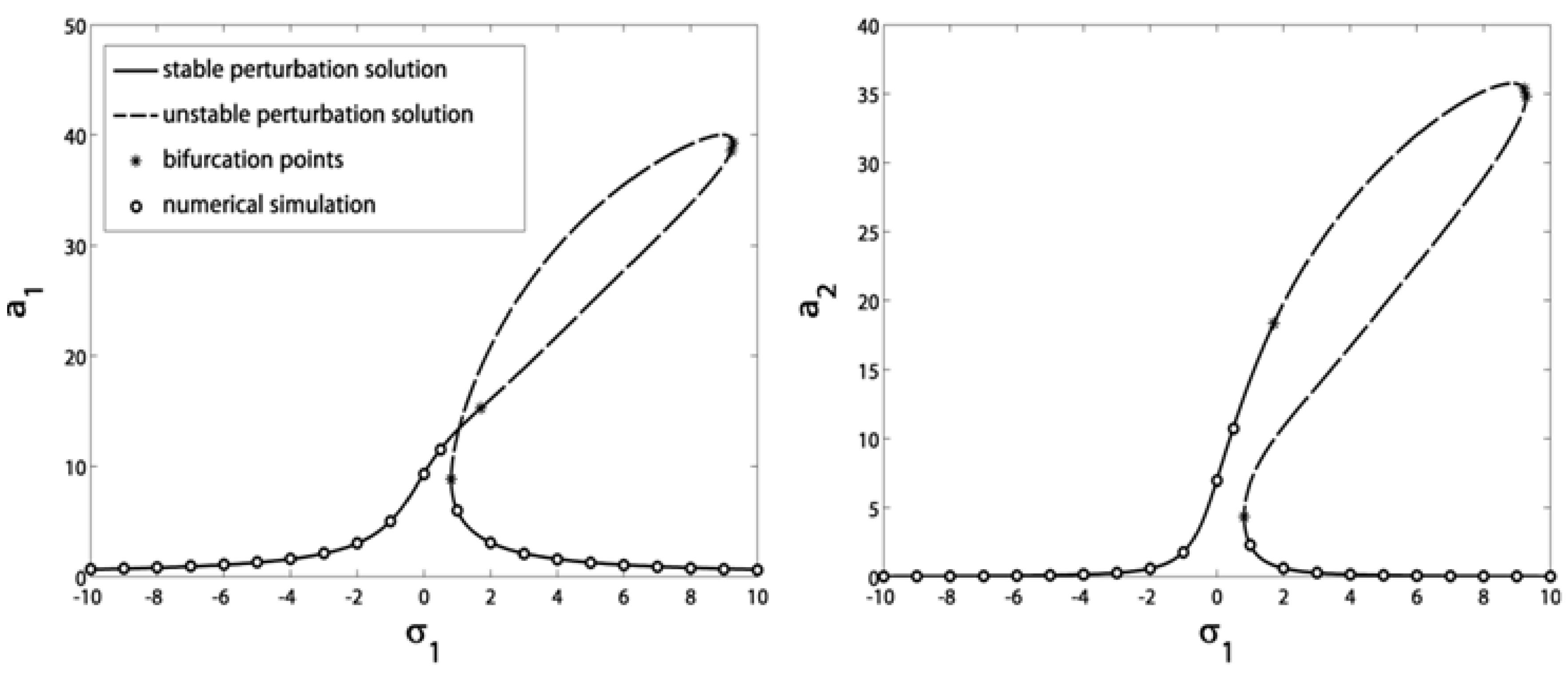
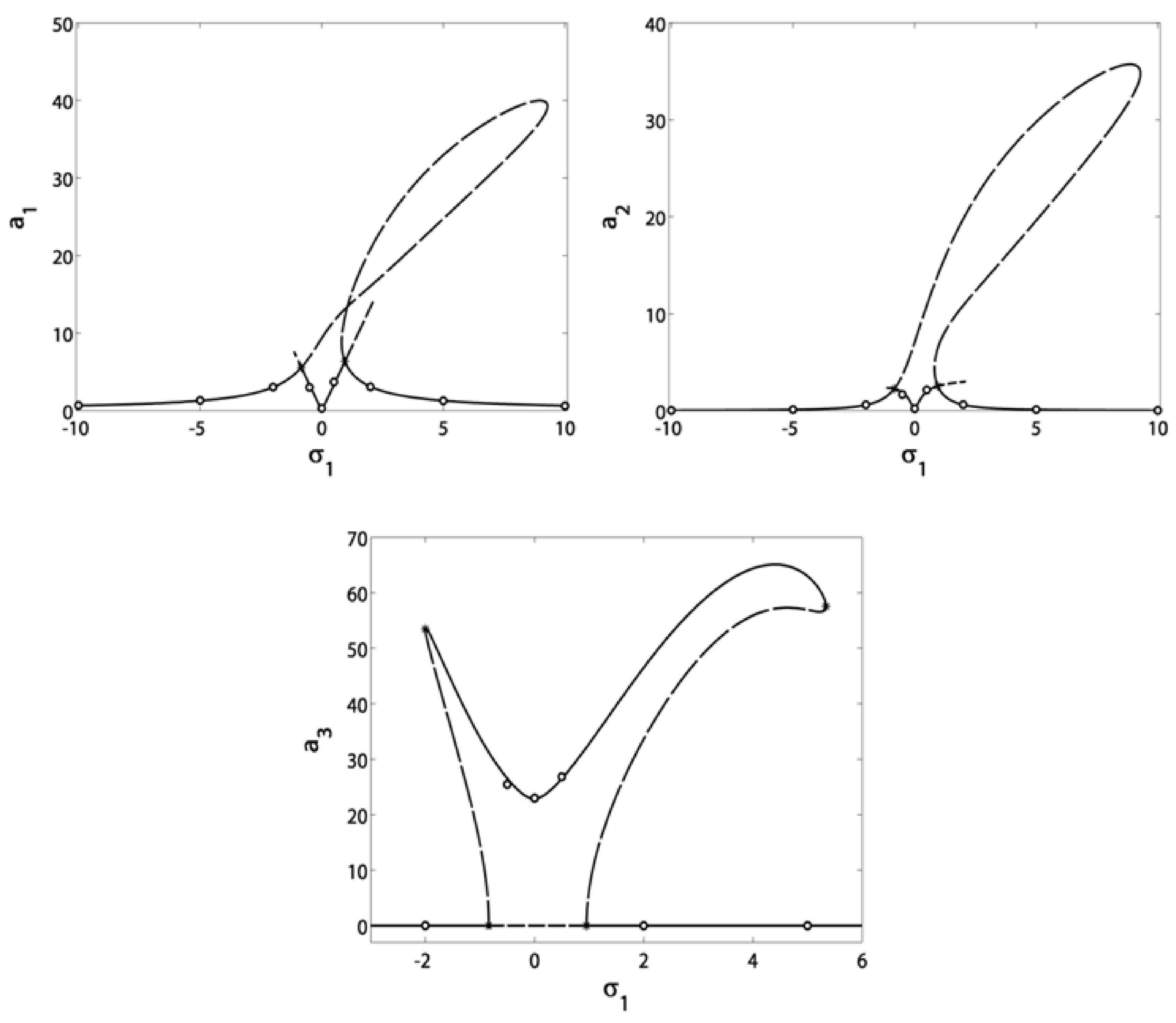
We are interested in studying how the rotating speed $\mathsf{\Omega }$ (${\sigma }_1=\mathsf{\Omega }-\omega$) affects the vibrational amplitudes of the blade and controller. Figure 5 shows the dependence of the blade vibrational amplitudes on the detuning ${\sigma }_1$ before control. For ${\sigma }_1>0$, it can be seen that the blade amplitudes increase and pass through SN points leading to jump phenomena, and pass through H points leading to stability switching. That is why we want to control the response in this region. Figure 6 depicts the same discussion in Figure 5 but with applying the saturation control algorithm at various combination values ${\tau }_1+{\tau }_2$. All SN and H points in Figure 5 have disappeared in Figure 6, while PF points have appeared to invert the blade amplitudes’ path to the V-shaped curve. This makes the blade leave the old response trajectory (before control) into a new V-curve trajectory. As seen in the figure, the blade amplitudes have been notched down to minimum values at ${\sigma }_1=0$ and they are not affected by changing the time delays combination ${\tau }_1+{\tau }_2$ within their safe constraint. On the other hand, the controller has amplitude peaks that have risen directly by increasing the time delays combination.

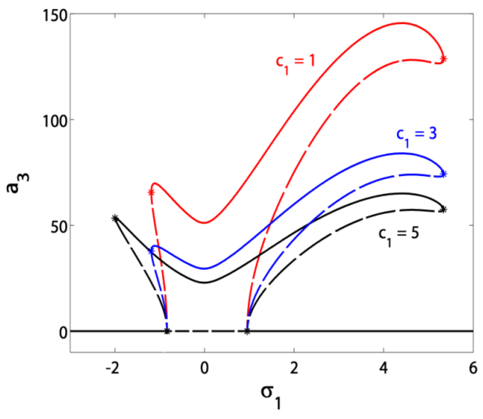
Figure 7 and Figure 8 have been plotted to demonstrate the effects of varying the control signal gain $c_1$ and the feedback signal gain $c_2$ on the blade and controller amplitudes response to ${\sigma }_1$ at ${\tau }_1+{\tau }_2=0.0025$. The steady-state form of Equations (11e) and (11f) shows that the amplitude $a_1$ (and so $a_2$) is only dependent on the parameter $c_2$ (in the case that $a_3\ne 0$). Thus, the parameter $c_1$ affects only the controller amplitude $a_3$ without any extra effects on the blade amplitudes ($a_1$ and $a_2$) as seen in Figure 7. It also shows that the controller amplitude is inversely proportional to $c_1$. On the other hand in Figure 8, increasing (decreasing) $c_2$ widens (tightens) the bandwidth of the V-shaped curve to extend the work of the controller.

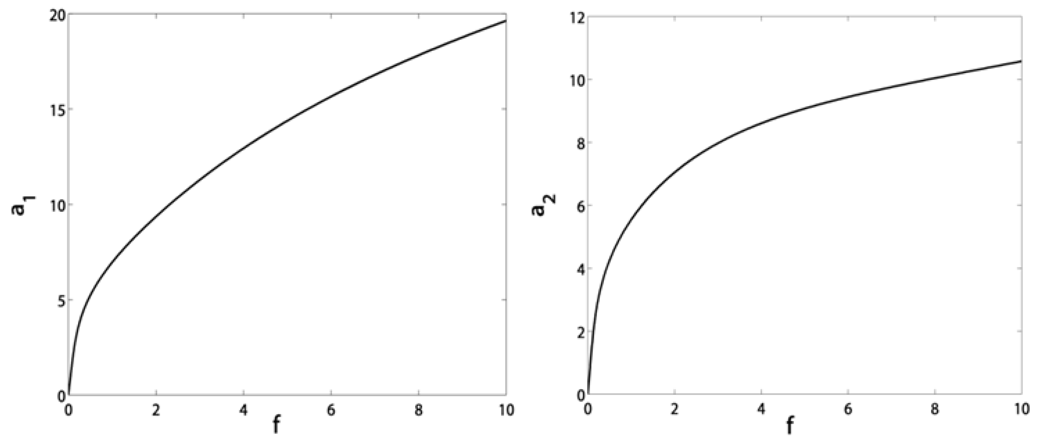
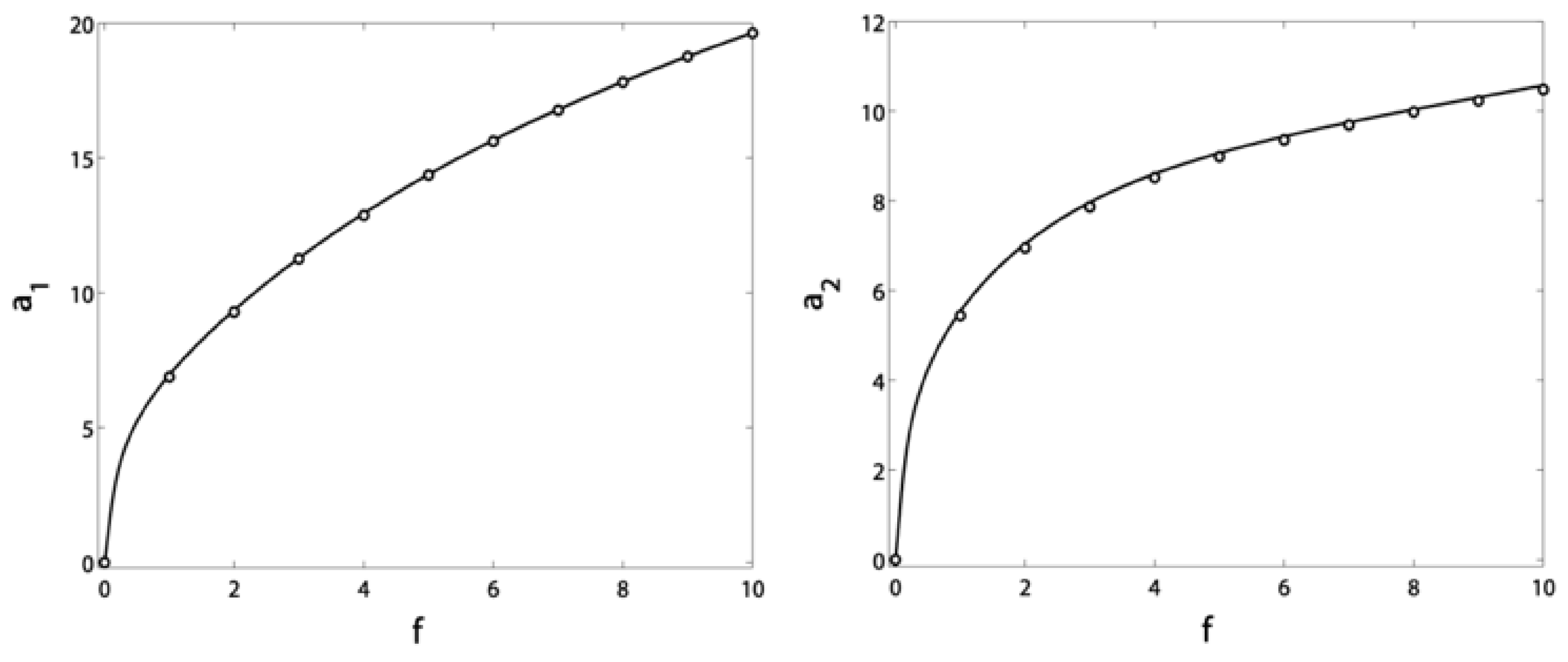
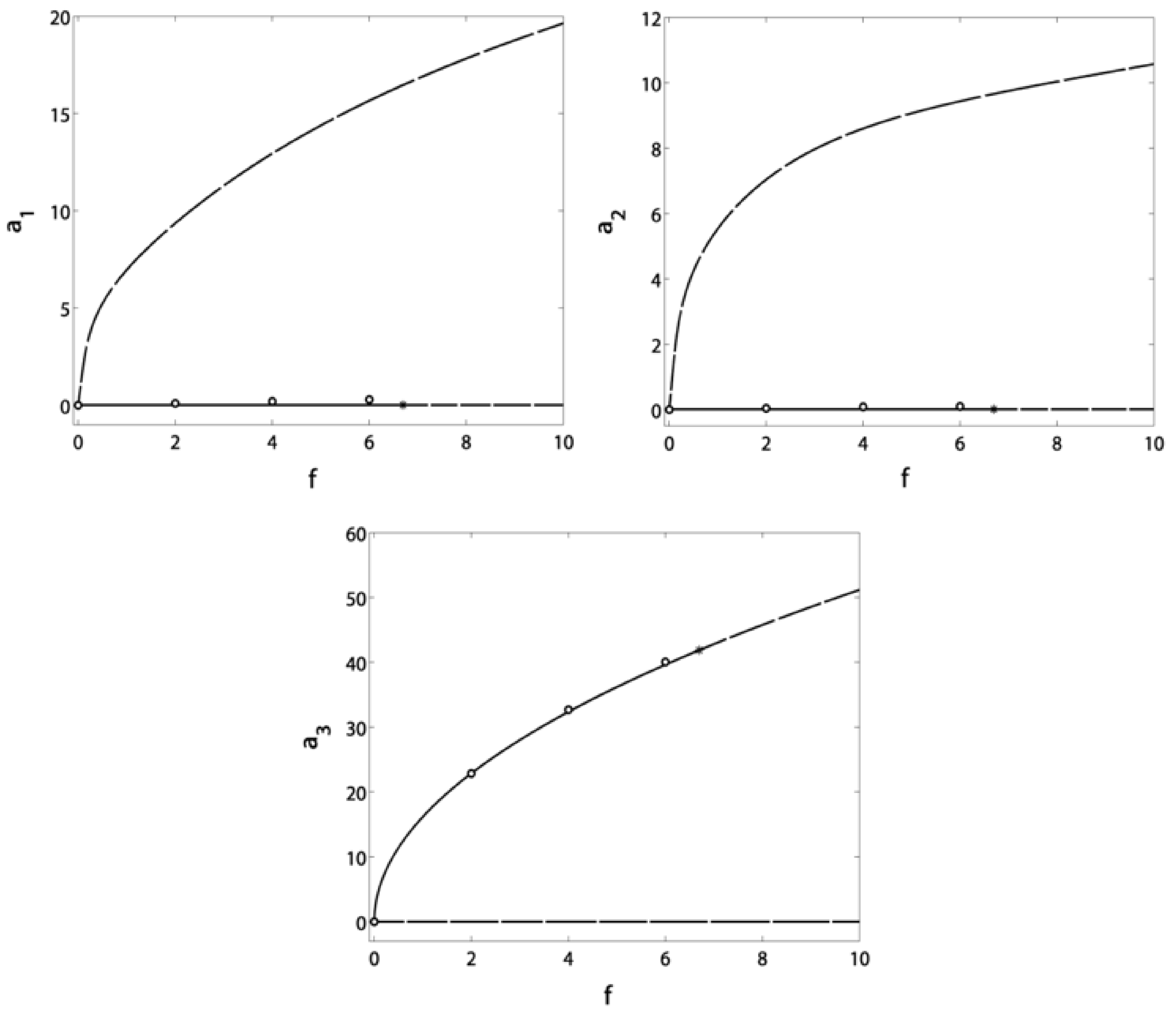
Figure 9 and Figure 10 clarify the response of the blade and controller amplitudes to the excitation force $f$ before and after control at ${\sigma }_1=0$. It is shown in Figure 9 that the increase in $f$ makes a sharp increase in the blade amplitudes before control. After control in Figure 10, we notice the saturation phenomenon where the blade vibrations are saturated at the zero level, which is the main advantage of NSC. The rest of the vibration energy is channeled to the controller, as shown. The main drawback, appearing due to the time delay, is that the force $f$ should not exceed the value $f\cong 6.5$; otherwise, the blade will pass through the H point and exhibit unstable motions.

3.2. Time Response and Phase Plane

The incoming figures show the blade responses to the time before and after control, besides the phase planes for indicating the blade equilibrium behavior after control. These figures are plotted using the fourth-order Runge–Kutta algorithm by numerically integrating Equation (2). Before control, the blade responses to time are shown in Figure 11, while Figure 12 presents the blade and controller time responses after control at zero time delays. We can see that the blade horizontal and vertical oscillations have been suppressed by about $97\%$ of their uncontrolled levels. Regarding the time delay effect, Figure 13 clarifies the blade and controller time responses after control at safe time delays (${\tau }_1+{\tau }_2=0.0025$). Here, the blade horizontal and vertical oscillations have been suppressed by about $96\%$ of their uncontrolled levels. This guides us to assure that the reduction ratio (with safe time delays) has decreased slightly where it cannot be noticed. In Figure 14, we impose unsafe time delays (${\tau }_1+{\tau }_2=0.005$) on the control process. The blade and controller oscillations have unstable waveforms meaning that the controller loses its efficiency in mitigating the blade vibrations as long as the time delays have passed the border line ${\tau }_1+{\tau }_2=0.0039$. All the steady-state oscillations are in the form of multi-limit cycles, as shown in the figure.

3.3. Verification of the Analytical Solutions

Here in this section, we present comparison figures (Figure 15, Figure 16, Figure 17 and Figure 18) to clarify the good agreement between the analytical and numerical solutions. It is also a verification of the analytical solutions approached by the multiple scales method.

4. Conclusions

In this research, rotating blade non-linear oscillations were reduced via a time-delayed non-linear saturation controller (NSC). This controller was excited by a positive displacement signal measured from the blade, while its output was the control force to be applied on the blade. Based on the saturation phenomenon, the blade vibrations could be saturated at a specific level forcing the rest of the energy to be transferred to the controller. The whole behavior was governed by a system of first-order differential equations gained by the method of multiple scales. Different responses were included to show the influences of time delay on the closed-loop control process. From this analysis, we could conclude the following items:

• The time delays constraint τ₁ + τ₂ < 0.0039 is a safe guarantee for stable blade vibrations after control.
• The bifurcation points (SN and H), that were present before control, were eliminated after control.
• After control, the bifurcation points (PF) have appeared to switch the blade speed response to a V-shaped curve, making it reach a minimum value at σ₁ = 0.
• The control gain c₁ affected only the controller without any extra effects on the blade amplitudes.
• The blade vibrations were saturated at zero level due to the saturation phenomenon, while vibration energy was channeled to the controller.
• The existence of the time delay diminished the excitation force’s stable range to make it not exceed a critical value; otherwise, the blade would pass through H point and exhibit unstable motions.
• This encourages us to suggest that the reduction ratio (with safe time delays) has decreased slightly where it cannot be noticed.
• Safe time delay occurrence has slightly reduced the vibration reduction ratio from about 97% to about 96% where it could not be noticed.
• The blade and controller exhibited multi-limit cycles as long as the time delays have passed the border line τ₁ + τ₂ = 0.0039.

References

- Yao, M.; Chen, Y.P.; Zhang, W. Nonlinear vibrations of blade with varying rotating speed. Nonlinear Dyn. 2012, 68, 487–504. [Google Scholar] [CrossRef]
- Wang, F.; Zhang, W. Stability analysis of a nonlinear rotating blade with torsional vibrations. J. Sound Vib. 2012, 331, 5755–5773. [Google Scholar] [CrossRef]
- Yao, M.; Zhang, W.; Chen, Y.P. Analysis on nonlinear oscillations and resonant responses of a compressor blade. Acta Mech. 2014, 225, 3483–3510. [Google Scholar] [CrossRef]
- Sina, S.; Haddadpour, H. Axial–torsional vibrations of rotating pretwisted thin walled composite beams. Int. J. Mech. Sci. 2014, 80, 93–101. [Google Scholar] [CrossRef]
- Wang, F.; Qu, Y. Period Doubling Motions of a Nonlinear Rotating Beam at 1:1 Resonance. Int. J. Bifurc. Chaos 2014, 24, 1450159. [Google Scholar] [CrossRef]
- Pešek, L.; Hajžman, M.; Ust, L.P.; Zeman, V.; Byrtus, M.; Brůha, J. Experimental and numerical investigation of friction element dissipative effects in blade shrouding. Nonlinear Dyn. 2014, 79, 1711–1726. [Google Scholar] [CrossRef]
- Hamed, Y.S.; Amer, Y.A. Nonlinear saturation controller for vibration supersession of a nonlinear composite beam. J. Mech. Sci. Technol. 2014, 28, 2987–3002. [Google Scholar] [CrossRef]
- Bian, X.; Chen, F.; An, F. Global Dynamics of a Compressor Blade with Resonances. Math. Probl. Eng. 2016, 2016, 3275750. [Google Scholar] [CrossRef] [Green Version]
- Kim, H.; Chung, J. Nonlinear modeling for dynamic analysis of a rotating cantilever beam. Nonlinear Dyn. 2016, 86, 1981–2002. [Google Scholar] [CrossRef]
- Li, X.; Hou, J.; Chen, J. An analytical method for Mathieu oscillator based on method of variation of parameter. Commun. Nonlinear Sci. Numer. Simul. 2016, 37, 326–353. [Google Scholar] [CrossRef]
- Luo, Z.; Wang, Y.; Zhai, J.; Zhu, Y. Accurate prediction approach of dynamic characteristics for a rotating thin walled annular plate considering the centrifugal stress requirement. J. Vibroeng. 2016, 18, 3104–3116. [Google Scholar] [CrossRef]
- Zhang, X.; Chen, F.; Zhang, B.; Jing, T. Local bifurcation analysis of a rotating blade. Appl. Math. Model. 2016, 40, 4023–4031. [Google Scholar] [CrossRef]
- Zhao, T.-Y.; Yuan, H.-Q.; Li, B.-B.; Li, Z.-J.; Liu, L.-M. Analytical Solution for Rotational Rub-Impact Plate under Thermal Shock. J. Mech. 2016, 32, 297–311. [Google Scholar] [CrossRef]
- Asghari, M.; Hashemi, M. The couple stress-based nonlinear coupled three-dimensional vibration analysis of microspinning Rayleigh beams. Nonlinear Dyn. 2016, 87, 1315–1334. [Google Scholar] [CrossRef]
- Cao, D.-X.; Liu, B.; Yao, M.; Zhang, W. Free vibration analysis of a pre-twisted sandwich blade with thermal barrier coatings layers. Sci. China Ser. E Technol. Sci. 2017, 60, 1747–1761. [Google Scholar] [CrossRef]
- Kandil, A.; Eissa, M. Improvement of positive position feedback controller for suppressing compressor blade oscillations. Nonlinear Dyn. 2017, 90, 1727–1753. [Google Scholar] [CrossRef]
- Farsadi, T.; Rahmanian, M.; Kayran, A. Geometrically nonlinear aeroelastic behavior of pretwisted composite wings modeled as thin walled beams. J. Fluids Struct. 2018, 83, 259–292. [Google Scholar] [CrossRef]
- Kandil, A.; El-Gohary, H. Investigating the performance of a time delayed proportional–derivative controller for rotating blade vibrations. Nonlinear Dyn. 2018, 91, 2631–2649. [Google Scholar] [CrossRef]
- Kandil, A.; El-Gohary, H.A. Suppressing the nonlinear vibrations of a compressor blade via a nonlinear saturation controller. J. Vib. Control 2016, 24, 1488–1504. [Google Scholar] [CrossRef]
- Khaniki, H.B. Vibration analysis of rotating nanobeam systems using Eringen’s two-phase local/nonlocal model. Phys. E Low-Dimens. Syst. Nanostruct. 2018, 99, 310–319. [Google Scholar] [CrossRef]
- Li, C.; Shen, Z.; Zhong, B.; Wen, B. Study on the Nonlinear Characteristics of a Rotating Flexible Blade with Dovetail Interface Feature. Shock. Vib. 2018, 2018, 4923898. [Google Scholar] [CrossRef]
- Yao, M.; Ma, L.; Zhang, W. Nonlinear Dynamics of the High-Speed Rotating Plate. Int. J. Aerosp. Eng. 2018, 2018, 1–23. [Google Scholar] [CrossRef] [Green Version]
- Gu, X.; Hao, Y.; Zhang, W.; Liu, L.; Chen, J. Free vibration of rotating cantilever pre-twisted panel with initial exponential function type geometric imperfection. Appl. Math. Model. 2019, 68, 327–352. [Google Scholar] [CrossRef]
- Heidari, M.; Arvin, H. Nonlinear free vibration analysis of functionally graded rotating composite Timoshenko beams reinforced by carbon nanotubes. J. Vib. Control 2019, 25, 2063–2078. [Google Scholar] [CrossRef]
- Niu, Y.; Zhang, W.; Guo, X.-Y. Free vibration of rotating pretwisted functionally graded composite cylindrical panel reinforced with graphene platelets. Eur. J. Mech. A/Solids 2019, 77, 103798. [Google Scholar] [CrossRef]
- Umerc, M.; Botto, D. Measurement of contact parameters on under-platform dampers coupled with blade dynamics. Int. J. Mech. Sci. 2019, 159, 450–458. [Google Scholar] [CrossRef]
- Yang, S.; Zhang, W.; Mao, J. Nonlinear vibrations of carbon fiber reinforced polymer laminated cylindrical shell under non-normal boundary conditions with 1:2 internal resonance. Eur. J. Mech. A/Solids 2019, 74, 317–336. [Google Scholar] [CrossRef]
- Yao, M.; Niu, Y.; Hao, Y. Nonlinear dynamic responses of rotating pretwisted cylindrical shells. Nonlinear Dyn. 2019, 95, 151–174. [Google Scholar] [CrossRef]
- Zhang, B.; Zhang, Y.-L.; Yang, X.-D.; Chen, L.-Q. Saturation and stability in internal resonance of a rotating blade under thermal gradient. J. Sound Vib. 2019, 440, 34–50. [Google Scholar] [CrossRef]
- Khosravi, S.; Arvin, H.; Kiani, Y. Vibration analysis of rotating composite beams reinforced with carbon nanotubes in thermal environment. Int. J. Mech. Sci. 2019, 164, 105187. [Google Scholar] [CrossRef]
- Han, H.; Liu, L.; Cao, D. Dynamic modeling for rotating composite Timoshenko beam and analysis on its bending-torsion coupled vibration. Appl. Math. Model. 2020, 78, 773–791. [Google Scholar] [CrossRef]
- Hamed, Y.; Albogamy, K.; Sayed, M. Nonlinear vibrations control of a contact-mode AFM model via a time-delayed positive position feedback. Alex. Eng. J. 2021, 60, 963–977. [Google Scholar] [CrossRef]
- Hamed, Y.S.; Albogamy, K.M.; Sayed, M. A proportional derivative (PD) controller for suppression the vibrations of the a contact-mode AFM model. IEEE Access 2020, 8, 214061–214070. [Google Scholar] [CrossRef]
- He, J.-H. Homotopy perturbation technique. Comput. Methods Appl. Mech. Eng. 1999, 178, 257–262. [Google Scholar] [CrossRef]
- He, J.-H. A coupling method of a homotopy technique and a perturbation technique for non-linear problems. Int. J. Non-Linear Mech. 2000, 35, 37–43. [Google Scholar] [CrossRef]
- He, J.-H. Homotopy perturbation method: A new nonlinear analytical technique. Appl. Math. Comput. 2003, 135, 73–79. [Google Scholar] [CrossRef]
- Noeiaghdam, S.; Dreglea, A.; He, J.-H.; Avazzadeh, Z.; Suleman, M.; Araghi, M.A.F.; Sidorov, D.; Sidorov, N.A. Error Estimation of the Homotopy Perturbation Method to Solve Second Kind Volterra Integral Equations with Piecewise Smooth Kernels: Application of the CADNA Library. Symmetry 2020, 12, 1730. [Google Scholar] [CrossRef]
- Hussain, S.; Shah, A.; Ayub, S.; Ullah, A. An approximate analytical solution of the Allen-Cahn equation using homotopy perturbation method and homotopy analysis method. Heliyon 2019, 5, e03060. [Google Scholar] [CrossRef] [Green Version]
- Javeed, S.; Baleanu, D.; Waheed, A.; Khan, M.S.; Affan, H. Analysis of Homotopy Perturbation Method for Solving Fractional Order Differential Equations. Mathematics 2019, 7, 40. [Google Scholar] [CrossRef] [Green Version]
- Nayfeh, A.H.; Mook, D.T. Nonlinear Oscillations; Wiley: New York, NY, USA, 1995. [Google Scholar] [CrossRef]
Figure 1.
Closed-loop control process of the rotating blade.
Figure 2.
Effect of the feedback signal delay on the blade and controller vibrational amplitudes at no control signal delay ().
Figure 3.
Effect of the control signal delay on the blade and controller vibrational amplitudes at no feedback signal delay ().
Figure 4.
Border line between stable and unstable amplitudes based on and values.
Figure 5.
Vibrational amplitudes of the blade in terms of the speed detuning before control.
Figure 6.
Vibrational amplitudes of the blade and controller in terms of the speed detuning at different combinations .
Figure 7.
The control signal gain effect on the controller amplitude at .
Figure 8.
The feedback signal gain effect on the blade and controller amplitudes at .
Figure 9.
Response of the blade amplitudes to the excitation force at before control.
Figure 10.
Response of the blade and controller amplitudes to the excitation force at and .
Figure 11.
The blade responses to time before control.
Figure 12.
The blade and controller responses to time at .
Figure 13.
Figure 14.
The blade and controller time responses and phase planes at .
Figure 15.
Verification of the blade vibrational amplitudes in terms of the speed detuning before control.
Figure 16.
Verification of the blade and controller vibrational amplitudes in terms of the speed detuning at .
Figure 17.
Verification of the blade amplitudes response to the excitation force at before control.
Figure 18.
Verification of the blade and controller amplitudes response to the excitation force at and .
Publisher’s Note: MDPI stays neutral with regard to jurisdictional claims in published maps and institutional affiliations. |
© 2021 by the authors. Licensee MDPI, Basel, Switzerland. This article is an open access article distributed under the terms and conditions of the Creative Commons Attribution (CC BY) license (http://creativecommons.org/licenses/by/4.0/).
Share and Cite
MDPI and ACS Style
Hamed, Y.S.; Kandil, A. Influence of Time Delay on Controlling the Non-Linear Oscillations of a Rotating Blade. Symmetry 2021, 13, 85. https://0-doi-org.brum.beds.ac.uk/10.3390/sym13010085
AMA Style
Hamed YS, Kandil A. Influence of Time Delay on Controlling the Non-Linear Oscillations of a Rotating Blade. Symmetry. 2021; 13(1):85. https://0-doi-org.brum.beds.ac.uk/10.3390/sym13010085
Chicago/Turabian StyleHamed, Yasser Salah, and Ali Kandil. 2021. "Influence of Time Delay on Controlling the Non-Linear Oscillations of a Rotating Blade" Symmetry 13, no. 1: 85. https://0-doi-org.brum.beds.ac.uk/10.3390/sym13010085
Note that from the first issue of 2016, this journal uses article numbers instead of page numbers. See further details here.