Using C++ to Calculate SO(10) Tensor Couplings

Bhagwagar, Azadan; Syed, Raza M.

doi:10.3390/sym13101871

Open AccessArticle

Using C++ to Calculate SO(10) Tensor Couplings

by

Azadan Bhagwagar

^1,† and

Raza M. Syed

^2,*,†,‡

¹

Department of Computer Science and Engineering, American University of Sharjah, Sharjah P.O. Box 26666, United Arab Emirates

²

Department of Physics, American University of Sharjah, Sharjah P.O. Box 26666, United Arab Emirates

^*

Author to whom correspondence should be addressed.

^†

These authors contributed equally to this work.

^‡

Current address: Department of Physics, Northeastern University, Boston, MA 02115-5000, USA.

Symmetry 2021, 13(10), 1871; https://0-doi-org.brum.beds.ac.uk/10.3390/sym13101871

Submission received: 8 August 2021 / Revised: 10 September 2021 / Accepted: 24 September 2021 / Published: 4 October 2021

(This article belongs to the Special Issue Symmetry, Collider Phenomenology and High Energy Physics)

Download

Browse Figure

Versions Notes

Abstract

:

Model building in

SO (10)

, which is the leading grand unification framework, often involves large Higgs representations and their couplings. Explicit calculations of such couplings is a multi-step process that involves laborious calculations that are time consuming and error prone, an issue which only grows as the complexity of the coupling increases. Therefore, there exists an opportunity to leverage the abilities of computer software in order to algorithmically perform these calculations on demand. This paper outlines the details of such software, implemented in C++ using in-built libraries. The software is capable of accepting invariant couplings involving an arbitrary number of

SO (10)

Higgs tensors, each having up to five indices. The output is then produced in LaTeX, so that it is universally readable and sufficiently expressive. Through the use of this software,

SO (10)

coupling analysis can be performed in a way that minimizes calculation time, eliminates errors, and allows for experimentation with couplings that have not been computed before in the literature. Furthermore, this software can be expanded in the future to account for similar Higgs–Spinor coupling analysis, or extended to include further

SO (N)

invariant couplings.

Keywords:

SO(10); C++; Higgs couplings

1. Introduction

The standard model of particle physics, including the strong and electroweak interactions comprising the group

SU {(3)}_{C} \times SU {(2)}_{L} \times U {(1)}_{Y}

, is highly successful [1,2,3,4,5]. One of the important challenges for particle physicists is to determine the underlying scheme where these forces are all unified. The aim of grand unified theories is three-fold: (1) To accomplish these unifications; (2) to provide an understanding of the three generations of quarks and leptons; (3) to provide an explanation of the hierarchy of their masses and of other properties. A more ambitious goal is to extend these ideas to encompass gravity, which requires the framework of superstring theory.

Grand unified models based on the gauge group

SO (10)

[6,7] have the most desirable features. They provide a framework for the unification of electroweak and strong interactions. They also allow for all the quarks and leptons of one generation to reside in a single

16

–plet irreducible spinor representation. Additionally, this complex representation contains a right-handed singlet state, needed for the generation of neutrino masses via the seesaw mechanism.

SO (10)

models also solve—in a relatively natural way—the doublet-triplet splitting problem without fine tuning. Next, they possess gauge interactions that conserve parity.

SO (10)

are aslo free from all gauge anomalies. Supersymmetric

SO (10)

models have the additional feature that they manage to unify the gauge couplings, and solve the hierarchy problem.

The Higgs sector of

SO (10)

models is largely unconstrained consisting of numerous possible representations. An avenue to the computation of the

SO (10)

couplings is via the decomposition of these in terms of

SU (5) \times U (1)

invariant couplings and then the further decomposition of them in terms of the

SU {(3)}_{C} \times SU {(2)}_{L} \times U {(1)}_{Y}

invariant couplings. The formalism to accomplish this was carried out in [8,9,10,11]. However, the explicit analyses of the couplings can be laborious and time consuming. For instance the complexity of computation involving large Higgs representations can be seen in the works of [12,13,14]. Thus various models employ elaborate Higgs representations to break the

SO (10)

grand unified theory (GUT) symmetry down to the Standard Model (SM) gauge group

SU {(3)}_{C} \times SU {(2)}_{L} \times U {(1)}_{Y}

. These consist of both small and large Higgs representations of

SO (10)

such as

10, 16 + \bar{16}, 45, 54, 120, 126 + \bar{126}, 144 + \bar{144}, 210

and

560 + \bar{560}

. This enormous freedom of choosing symmetry breaking patterns allows one to construct

SO (10)

models with natural splitting of Higgs doublets and Higgs triplets to accomplish electroweak symmetry breaking [12,13,14,15] and models with a one-scale breaking of

SO (10)

GUT symmetry [16,17,18,19,20]. However, there are restrictions on the Higgs content of a GUT model, such as the strict proton decay limits [21,22]. There are two commonly used symmetry breaking paths: One through the

SU (5) \times U (1)

maximal subgroup [8,9,10,11,23,24] and the other through the

SU (4) \times SU {(2)}_{L} \times SU {(2)}_{R}

maximal subgroup [25,26].

The Higgs-Higgs interactions, appearing in supersymmetric and non-supersymmetric

SO (10)

models, are necessary to break the GUT and electroweak symmetries. Additionally, a thorough study of higher dimensional operators arising from three point, four point and higher Higgs-Higgs Interactions and matter-Higgs interactions is necessary to explore physics beyond the SM. For example, from matter-Higgs interactions, a top-down approach [14] has been used to find dimension five, seven and nine

B - L = - 2

operators within the supersymmetric

SO (10)

grand unification framework. This is in stark contrast to the bottom-up approach that exists prominently in the literature. These

B - L

violating operators are important in the investigation of seesaw neutrino masses, baryogenesis, proton decay and

n - \bar{n}

oscillations.

In this paper, we use the techniques (see Appendix B.4) developed in [8,9,11] for the analysis of such

SO (2 N)

invariant interactions which allows a full exhibition of the

SU (N)

invariant content of tensor representations. In particular, in this paper, we focus on the analytic determination of

SO (10)

tensor interactions in terms of irreducible

SU (5)

fields. It would then be very straightforward to expand all the

SU (5)

invariants in terms of SM group invariants using the particle assignments. We wish to point out that our approach here is field theoretic rather than group theoretic [27,28] or other technique [29,30]. Our method is specially suited for the computation of

SO (N)

tensor couplings.

Manually preforming such tensor calculations can be a time-consuming endeavor that can very easily lead to errors. There are numerous intermediate calculations, each posing the risk of making an error, which may propagate throughout, affecting the final result. Therefore, there exists a compelling argument to use computer software to perform these calculations automatically, as proposed in this paper.

This C++ program allows users to perform Higgs-Higgs

SO (10)

coupling calculations rapidly and automatically, reducing the time needed to complete them and eliminating calculation errors.

With this program, the user is able to enter a coupling via a simple text-based interface. Next, the user is provided with the final normalized output, in a LaTeX format, which can easily be added to a user’s publication. Further, the user is allowed to enter an arbitrary number of tensors in an

SO (10)

invariant and can name their indices and tensors as needed. The maximum number of indices a single tensor can have is 5.

Furthermore, to ensure the correctness of the algorithm when applied to couplings not previously attempted in the literature, manual hand calculations were evaluated for certain terms and were successfully matched to the program output.

This program can be easily extended to account for Higgs–Spinor couplings [31], as well as other

SO (N)

couplings.

The code is available to download https://github.com/AHB99/tensor-coupling-program/releases (accessed on 13 September 2021).

There exists a variety of software packages for Lie algebra related computations used in grand unified models that are based on various classical and exceptional groups. Here are some examples. LieART 2.0 [32] uses a Mathematica library to perform various computations such as tensor product decomposition and subalgebra branching of irreducible representations. SARAH 4 [33] also exploits a Mathematica library that carries out calculations used in the study of supersymmetric and non-supersymmetric grand unified models, particularly, the full two-loop renormalization group equations for a supersymmetric theory. CleGo [34] package uses OCaml programming language to determine Clebsch–Gordan coefficients of irreducible tensor product representations of Lie algebras

A - G

. FeynRules 2.0 [35] is a Mathematica package that derives Feynman rules from the Lagrangian of the Standard Model, Minimal Supersymmetric Standard model and their numerous extensions. These software packages rely extensively on standard group theoretic methods and display different degrees of generality. As mentioned earlier, our C++ code uses the more intuitive field theoretic formalism for the analytic decomposition of the

SO (10)

invariants of arbitrary order in terms of

SU (5)

invariants exhibiting their precise tensorial structure and Clebsch–Gordan coefficients. Our computer program is complementary to the existing software packages.

The paper is organized as follows. Section 2 contains a detailed breakdown of the computer algorithm to provide readers with an overview of how the code is designed. Section 3 provides sample calculation output and Section 4 discusses the significance of our algorithm. To fully appreciate and understand the properties associated with the

SO (N)

groups, we provide a thorough presentation of these groups in the appendices. Specifically, we discuss vector and tensor representations of

SO (N)

group and aspects of

SO (N)

gauge theory in Appendix A.

SO (2 N)

group algebra in

SU (N)

basis, branching rules for

SO (2 N)

into

SU (N) \times U (1)

irreducible representations and its specialization to

SO (10)

case are explained in Appendix B. We show explicitly the technique to decompose

SO (2 N)

tensor invariants in terms of

SU (N)

tensor invariants in Appendix B.4. This technique (The Basic Theorem) uses a unique set of reducible

SU (N)

tensors in terms of which the

SO (2 N)

invariants have a straight forward decomposition. The Basic Theorem is specially useful for couplings involving large tensor representations and is central to the computation of any

SO (N)

invariant couplings.

SO (10)

tensors expressed in terms of

SU (5)

irreducible tensors with canonically normalized kinetic energy terms are exhibited in Appendix B.5. In Appendix B.6, we identify

SU {(3)}_{C} \times SU {(2)}_{L} \times U {(1)}_{Y}

singlets,

SU {(2)}_{L}

doublets and

SU {(3)}_{C}

triplets in

SU (5)

fields.

2. Materials and Methods

The program evaluates tensor couplings from input to their final normalized form. Internally, it is executed through various functions of the Product Resolver class, which stores all the intermediate terms during the calculation. It is based on the algorithm developed in Appendix B.4.

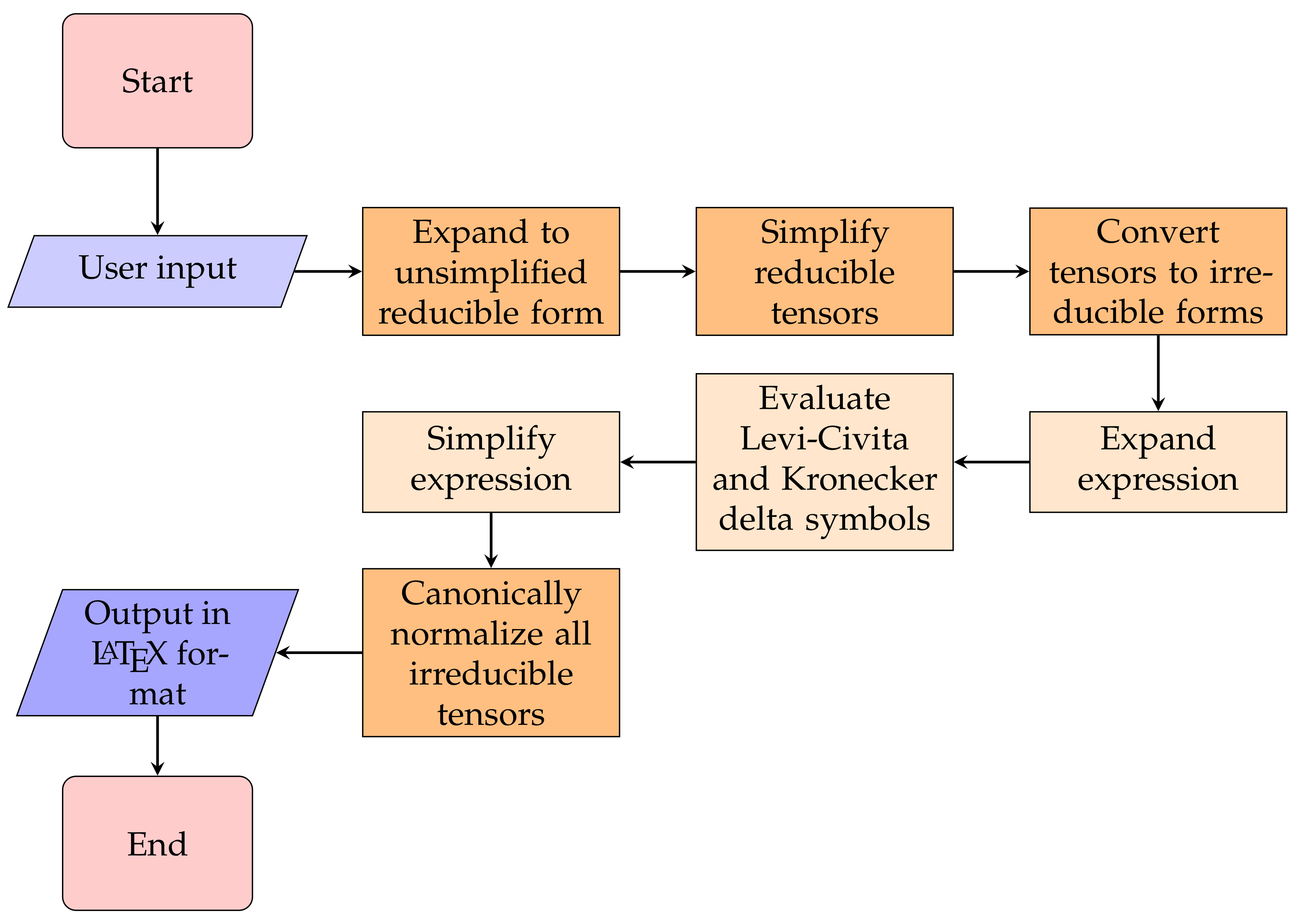
In brief, first the user inputs the original tensor coupling. This coupling is expanded to all its unsimplified reducible tensor terms. Then, all the reducible tensor terms are simplified by reordering the indices, accounting for anti-symmetry, and renaming indices if valid. Next, each reducible tensor term is substituted for its corresponding irreducible tensor expression. This expression is then expanded out fully. All Levi-Civita tensors are evaluated, following which the expression is simplified using the Kronecker Deltas and further properties of irreducible tensors. Then, all simplified irreducible tensor terms are further simplified by renaming if valid. Finally, these terms are substituted for their related normalized tensor term expressions, and the final expression is determined, to be output in LaTeX format. See Figure 1.

2.1. Input Phase

The user inputs a tensor coupling in the format “X_{/i/j/k}Y_{/i/j/k}…” where “X” and “Y” are labels for tensors and “/i/j/k” are labels for index names. The input is parsed using the standard C++ regex library. A regex expression is hard-coded to tokenize the tensors and the indices each. The Product Resolver class uses the following method:

void parseInput (std :: string input);

2.2. Generation Phase

All the initial generated reducible tensor terms can be determined by the following pattern. If one were to take a binary number where each binary digit corresponds to each unique index of the input tensor, and then increment the binary number from 0 to

2^{n} - 1

(where n is the number of unique indices), each binary number would correspond to a generated term. A term can be developed by the rule where for each binary digit, the corresponding index in that position will have its first occurrence barred if the binary digit is 1, or unbarred if it is 0. The function is as follows:

void generateAllUnsimplifiedReducibleTensorTerms ();

2.3. Simplification of Reducible Tensor Term Expression Phase

Now we have all the raw, generated reducible tensor terms, we may simplify them. This phase is based on the idea of tensor terms having similar “structure”. Two terms have the same “structure” if, assuming they have the same number of tensors, every tensor in every corresponding position has the same label and number of barred and unbarred indices. Only once two tensor terms have the same “structure” can the possibility of a rename operation leading to equality between them be considered. Currently, the generated tensor terms have their indices unordered, with no grouping of barred and unbarred indices. So firstly, each reducible tensor term has its indices reordered, accounting for anti-symmetry, by the below algorithm. The function is as follows:

void simplifyReducibleTensorTerms ();

2.3.1. Reordering of Reducible Tensor Term Indices

The algorithm is a modified implementation of bubble sorting, accounting for grouping of barred/unbarred indices, as well as anti-symmetry, acting on each Tensor. By the end, the tensors will have their barred indices grouped to the left, and unbarred indices grouped to the right, with each group ordered in ascending order of index names.

2.3.2. Sorting Tensor Terms

The tensor terms need to now be sorted in a uniform manner so that it becomes obvious to identify terms with the same “structure”, as defined above. We require sorting to be done first by tensor labels (alphabetically), then by number of indices, and then by number of barred indices

After sorting, the tensor terms are transferred to a separate container of simplified reducible tensor terms, checking to see if an addition or rename operation can be done with any existing simplified term first. The rename operation is detailed below

2.3.3. Renaming of Reducible Tensor Term Indices (Ignoring Commutativity) Algorithm

The algorithm takes two tensor terms, an Attempt Term that we are will be manipulating and renaming, as well as a Source Term, which will not be modified and is what the Attempt Term will be manipulated to match, if possible. It outputs a Renamed Term if the operation was successful, that, once its indices are reordered, will be identical to the Source Term (excluding coefficients, which are to be added). Moreover, the algorithm makes use of the concept of “zones”, which are either unbarred or barred groups of indices in a tensor. Tensor terms with the same “structure” will also have the same “zones”, and hence when deciding whether a rename operation is possible, we only have to focus on mapping each “zone” of the Attempt Term to the Source Term.

The algorithm assumes the Source Term and Attempt Term have their indices grouped as barred/unbarred and each group is ordered ascendingly, and that their tensors are sorted. The handling of commutativity, for tensor terms that retain identical structure upon permutations, is not considered in this algorithm.

2.3.4. Renaming of Reducible Tensor Term Indices (Accounting for Commutativity) Algorithm

This algorithm deals with the concept of “ambiguity” of tensor terms. This is a characteristic of a tensor term where it is possible to permute the ordering of the tensors within the term (due to the commutativity of tensors) and still retain identical “structure” (as defined above). This requires special consideration as the above Renaming Algorithm focuses on trying to equate corresponding “zones” in the Source and Attempt Terms based on position, so when such permutations are possible, the algorithm may fail to find a legal rename mapping for one arbitrary permutation while it may have been possible in another.

Hence, we need to exhaust every single possible permutation of “ambiguous” tensor terms. Specifically, we deal with the concept of “ambiguous zones”, which are groups of tensors within a tensor term that cause the “ambiguity” property (there can be multiple “ambiguous zones” within a single tensor term)

Ambiguity Detection:

During the rename operation, if a Source Term (and hence it’s matching structure Attempt Term) is found to be ambiguous, then we must generate all possible permutations of the ambiguous zones of the Attempt Term, attempt to rename them to the Source Term, and if even 1 successful rename exists, that must be chosen and applied. Only failing this do we conclude no possible rename exists. To generate all these permutations of the Attempt Term, we first must locate all such zones.

Finding all ambiguous zone locations and sizes:

Once we have the locations and sizes of all ambiguous zones of a tensor, we can generate all the permutations of the locations of all the ambiguous zones. This will be stored in a vector (the overall container) of vectors (for each zone) of vectors (for each permutation) of integers (the locations). For uniformity, we will consider each zone’s locations start from 0, and offset it with the actual location later.

Finding all permutations of the locations for all ambiguous zones:

Now, given this information, we can generate the tensor terms. However, we must consider the fact that for tensor terms with multiple ambiguous zones, we must generate all combinations of all the possible permutations of the ambiguous zones. For example, if a tensor term has 2 ambiguous zones, we must not permute the first zone and exhaust all the permutations of the second zone. Once we have exhausted them, only then can we proceed with the next permutation of the first zone, but again pause as we exhaust all the permutations of the second zone. This logic is expanded to the general case in the algorithm below.

Finding all permutations of the tensor terms for all ambiguous zones:

Now we permute the actual tensor terms in the locations to achieve all possible permutations to test out.

2.3.5. Simplification of Reducible Terms Algorithm

Now, we put all the algorithms together to simplify the raw, generated reducible tensor terms. The Product Resolver class contains within itself a vector of the raw, unsimplified terms, as well as the simplified terms.

Reorder the indices of all terms, alphabetically.
Sort the tensors of all terms, as defined above.
Iterate over all unsimplified terms:
(a)
Iterate over all simplified terms:
i.
If the current unsimplified (Attempt Term) and simplified (Source Term) terms have the same structure, attempt to rename them.
ii.
If the rename is successful, reorder the indices of the Re-named Term.
iii.
Check if the Renamed Term is identical to the Source Term. (Theoretically, this must always be true, as else the rename operation would not have been successful). If so, add the coefficient of the Renamed Term into the Source Term. Break iteration over the simplified terms.
(b)
If all simplified terms were iterated over with no successful matches, add the current unsimplified term to the vector of simplified terms. (It could not be simplified with any existing simplified term).
Erase all simplified tensor terms with a coefficient of 0

By the end of this stage, we have a vector of all simplified, reducible tensor terms.

2.4. Reduction of Reducible Tensor Terms to Irreducible Tensor Terms Phase

In this phase, we will first substitute the simplified, reducible tensors with their corresponding (pre-determined) expressions written in terms of irreducible tensors, Kronecker Deltas, and Levi-Civita tensors. We will then expand out these expressions, expand the Levi-Civita tensors, and then simplify the expression using the properties of Kronecker Deltas, Symmetric-Asymmetric irreducible tensors, and the ability to rename the indices of irreducible tensors and add them.

This phase will make use of the Math Expression class, which resembles a typical algebraic expression, composed of algebraic terms from the Math Expression Term class. The Math Expression Term will serve as a more complex form of the Tensor Term class used in previous phases, as it now will contain various mathematical objects. There are also self-explanatory classes for Deltas, Levi-Civitas, Irreducible Tensors, and Coefficients. The function is as follows:

void fullyReduceTensorTerms ();

2.4.1. Substitutions of Reducible Tensors for Expressions with Irreducible Tensors Algorithm

Given the Source Reducible Tensor, find the number of indices it contains.
Based on the number of indices, choose the correct substitution sub-category
In the chosen substitution sub-category, given the Source Reducible Tensor, find the number of barred indices it contains
Based on the number of barred indices of this sub-category (of number of indices), return the corresponding substituted Math Expression

The terms are then expanded by multiplication.

2.4.2. Multiplication of Levi-Civita Tensors Algorithm

Iterate for every Math Expression Term in a Math Expression:
(a)
If there is more than 1 Levi-Civita:
i.
If there are 3 or more Levi-Civitas, group the Levis based on number of common indices
ii.
Create a temporary Math Expression for the full Delta Expression
iii.
Iterate while there exists atleast one pair of Levis:
A.
Expand the pair into this temporary.
B.
Delete the pair
iv.
Multiply the original term with the full Delta Expression, and ap-pend this to the final result Math Expression.
v.
Set the original term to 0.
vi.
Delete all terms with 0 coefficient

2.4.3. Simplification of Expression by Kronecker Deltas Algorithm

Iterate for every term:
(a)
Sum over the indices of the Deltas.
(b)
Check for possibility of the deltas cancelling out the term. If so, move on to the next term.
(c)
Rename the indices of the irreducible tensors by using the Deltas.
(d)
Solve identical Deltas and modify the coefficient accordingly.
Erase all terms with coefficient 0.

2.4.4. Simplification of Expression by Renaming Indices of Irreducible Tensors (Accounting for Commutativity)

While before the concept of “zones” related to barred versus unbarred indices, now “zones” relates to upper versus lower indices.
While before the concept of “structure” (and hence “ambiguity”) related to whether 2 reducible tensors have the same label, number of indices, and number of barred indices, now “structure” relates to whether 2 irreducible tensors have the same bar state, field, symmetric property, and number of upper and lower indices.
While before the sorting of the reducible tensor terms was by (in ascending order) label, then by number of indices, and then by number of barred indices, now the sorting of the irreducible tensor terms is (in ascending order) by field, then by symmetric property, then by bar state, then by number of upper indices, and then by number of lower indices.
A Single Levi-Civita tensor may survive after simplification and also must be considered in the renaming process. It is considered as its own unique “zone”.

2.4.5. Overall Reduction Phase

Iterate for every Math Expression Term:
(a)
Substitute the reducible tensor terms for the appropriate Math Expressions containing irreducible tensors, Levi-Civitas, and Deltas.
(b)
Multiply and expand all the substituted expressions.
(c)
Multiply the Levi-Civitas of each term and expand the expression.
(d)
Simplify the overall expression by the properties of Kronecker Deltas.
(e)
Simplify the overall expression by the property of Symmetric and Asymmetric Irreducible tensors that share 2+ indices.
(f)
Simplify the overall expression by the renaming the indices of the expression.
(g)
Multiply the overall expression with the original coefficient from the reducible tensor term.
(h)
Append this result to the overall Math Expression of the final result.
Simplify this final result by renaming the indices of the expression
(a)
(This step is repeated because before it was only considered within each expression that arose from a reducible tensor term, whereas now it is considering all simplified expressions from all the reducible tensor terms.)
Multiply the overall expression with the coefficient that arose from expanding the initial user input to the reducible tensors (of the form $\frac{1}{2 (N u m b e r O f I n d i c e s)}$ ).

2.5. Normalization of Irreducible Tensors to Normalized Tensors Phase

In this final phase, we substitute the irreducible tensors with the corresponding normalized tensors, including their coefficients. This is similar to the step in the previous phase where we substituted the reducible tensors for their respective expressions. Each substitution is a unique function due to its coefficients, however the general procedure is outlined below.

For a given irreducible tensor of a Math Expression Term:
Create a normalized tensor and transfer the indices exactly as they are from the irreducible tensor.
Multiply the whole Math Expression Term by the required coefficient.
Erase the Irreducible Tensor from the Math Expression Term.

This process is repeated for every irreducible tensor in every Math Expression Term in the result expression. No further simplification occurs here because all simplification has been completed before this. Hence, we arrive at our final result. The function is as follows:

void normalizeIrreducibleTensorTerms ();

2.6. Output Phase

Every component in the result, be it a Delta, Normalized tensor, Coefficient, etc., has a representation in LaTeX designed for it, and hence printing a term simply calls all these functions in turn, and printing an expression calls the printing of each term. The function is as follows:

void printMathExpressionAsLaTeX ();

3. Results

The computer program outputs results in LaTeX format that can be easily included in a publication, as it has been done in Section 3.1, Section 3.2 and Section 3.3. The original

SO (10)

coupling inputs are mentioned along with their respective processed results in their final format. Some of these couplings have not previously been demonstrated in the literature, proving the generalized capabilities of the software.

The normalizations of

SU (5)

fields are displayed in Appendix B.5. Here the H—fields represent

SU (5)

irreducible tensors with canonically normalized kinetic energy terms.

3.1. Quadratic Couplings

126 × 126

X_{μ 1 μ 2 μ 3 μ 4 μ 5} X_{μ 1 μ 2 μ 3 μ 4 μ 5} = + 2 H^{(\bar{126})} {\bar{H}}^{(126)} + H_{(S)}^{m p (\bar{126})} H_{m p (S)}^{(126)} + H^{p q (126)} H_{p q}^{(\bar{126})} + \frac{1}{6} H_{l m}^{i j k (\bar{126})} H_{i j k}^{l m (126)} + H_{m}^{j k (126)} H_{j k}^{m (\bar{126})} + 2 H^{k (\bar{126})} H_{k}^{(126)}

3.2. Cubic Couplings

3.2.1. 210 × 210 × 210

X_{μ 1 μ 2 μ 3 μ 4} X_{μ 3 μ 4 μ 5 μ 6} X_{μ 5 μ 6 μ 1 μ 2} = + \frac{1 \sqrt{2}}{2} H^{p (210)} H_{n}^{(210)} H_{p}^{n (210)} - \frac{1 \sqrt{15}}{5} H^{(210)} H^{p (210)} H_{p}^{(210)} - \frac{1 \sqrt{6}}{48} ϵ^{i j k l o} H_{o}^{(210)} H_{k l n}^{m (210)} H_{i j m}^{n (210)} + \frac{1 \sqrt{2}}{12} ϵ^{i j k l o} H_{o}^{(210)} H_{i m}^{(210)} H_{j k l}^{m (210)} + \frac{1 \sqrt{6}}{48} ϵ^{i j k l o} H_{o}^{(210)} H_{k l}^{(210)} H_{i j}^{(210)} - \frac{1 \sqrt{6}}{48} ϵ_{i j m n o} H^{o (210)} H_{l}^{i j k (210)} H_{k}^{l m n (210)} - \frac{1 \sqrt{2}}{12} ϵ_{i j m n o} H^{o (210)} H^{l m (210)} H_{l}^{i j n (210)} + \frac{1 \sqrt{6}}{48} ϵ_{i j m n o} H^{o (210)} H^{i j (210)} H^{m n (210)} + \frac{1 \sqrt{3}}{6} H_{l}^{i j k (210)} H_{k n}^{l m (210)} H_{i j m}^{n (210)} + \frac{1}{6} H_{l}^{i k n (210)} H_{i m}^{(210)} H_{k n}^{l m (210)} - \frac{1 \sqrt{2}}{12} H_{k}^{m (210)} H_{n}^{i j k (210)} H_{i j m}^{n (210)} - \frac{1 \sqrt{6}}{36} H_{k}^{m (210)} H_{m}^{i j k (210)} H_{i j}^{(210)} + \frac{1 \sqrt{2}}{12} H_{n}^{l (210)} H_{l}^{i j m (210)} H_{i j m}^{n (210)} - \frac{1 \sqrt{6}}{36} H^{i j (210)} H_{n}^{m (210)} H_{i j m}^{n (210)} + \frac{1 \sqrt{2}}{18} H^{i k (210)} H_{k}^{m (210)} H_{i m}^{(210)} - \frac{1}{6} H^{i k (210)} H_{k n}^{j m (210)} H_{i j m}^{n (210)} + \frac{5 \sqrt{3}}{36} H^{k n (210)} H_{j m}^{(210)} H_{k n}^{j m (210)} + \frac{1 \sqrt{3}}{12} H_{l}^{i j k (210)} H_{i j}^{m n (210)} H_{k m n}^{l (210)} - \frac{1 \sqrt{15}}{20} H^{(210)} H^{k m (210)} H_{k m}^{(210)} + \frac{1 \sqrt{3}}{36} H_{k l}^{i j (210)} H_{m n}^{k l (210)} H_{i j}^{m n (210)} - \frac{1 \sqrt{2}}{6} H_{i}^{n (210)} H_{k l}^{i m (210)} H_{m n}^{k l (210)} + \frac{1 \sqrt{15}}{60} H^{(210)} H_{k l}^{m n (210)} H_{m n}^{k l (210)} - \frac{1 \sqrt{3}}{18} H_{m}^{l (210)} H_{i}^{n (210)} H_{l n}^{i m (210)} + \frac{7 \sqrt{2}}{54} H_{n}^{m (210)} H_{m}^{i (210)} H_{i}^{n (210)} - \frac{1 \sqrt{15}}{60} H^{(210)} H_{l}^{m (210)} H_{m}^{l (210)} - \frac{1 \sqrt{15}}{30} H^{(210)} H^{(210)} H^{(210)} + \frac{1 \sqrt{3}}{9} H_{j l}^{i k (210)} H_{k n}^{l m (210)} H_{i m}^{j n (210)}

3.2.2. 210 × 126 × 210

X_{μ 1 μ 2 μ 3} Y_{μ 2 μ 3 μ 4 μ 5 μ 6} Z_{μ 1 μ 4 μ 5 μ 6} = + \frac{1 \sqrt{15}}{60} H_{m n}^{(120)} H^{q (210)} H_{q}^{m n (126)} + \frac{1 \sqrt{5}}{20} H_{n q}^{(120)} H^{q (210)} H^{n (\bar{126})} + \frac{1 \sqrt{30}}{480} ϵ^{i j k o p} H_{o p}^{(120)} H_{i l m}^{n (210)} H_{j k n}^{l m (126)} + \frac{1 \sqrt{10}}{480} ϵ^{i j k o p} H_{o p}^{(120)} H_{l m}^{(210)} H_{i j k}^{l m (126)} + \frac{1 \sqrt{15}}{120} ϵ^{i j k o p} H_{o p}^{(120)} H_{i j m}^{n (210)} H_{k n}^{m (\bar{126})} + \frac{1 \sqrt{5}}{240} ϵ^{i j k o p} H_{o p}^{(120)} H_{i m}^{(210)} H_{j k}^{m (\bar{126})} + \frac{1 \sqrt{5}}{240} ϵ^{i j k o p} H_{o p}^{(120)} H_{i j k}^{n (210)} H_{n}^{(126)} - \frac{1 \sqrt{15}}{240} ϵ^{i j k o p} H_{o p}^{(120)} H_{i j}^{(210)} H_{k}^{(126)} - \frac{1 \sqrt{5}}{20} H_{n q}^{(120)} H_{i}^{n (210)} H_{(S)}^{i q (\bar{126})} + \frac{1 \sqrt{30}}{120} H_{m n}^{(120)} H_{i j}^{m n (210)} H^{i j (126)} + \frac{1 \sqrt{5}}{60} H_{n r}^{(120)} H_{i}^{n (210)} H^{i r (126)} + \frac{1 \sqrt{6}}{40} H_{q r}^{(120)} H^{(210)} H^{q r (126)} - \frac{1 \sqrt{10}}{40} H_{l m}^{(120)} H^{l m (210)} {\bar{H}}^{(126)} - \frac{1 \sqrt{15}}{60} H_{q}^{o p (120)} H^{q (210)} H_{o p}^{(\bar{126})} + \frac{1 \sqrt{15}}{30} H^{j (120)} H^{q (210)} H_{j q (S)}^{(126)} - \frac{1 \sqrt{15}}{60} H^{o (120)} H^{q (210)} H_{o q}^{(\bar{126})} - \frac{1 \sqrt{30}}{120} H_{k}^{i j (120)} H_{i l m}^{n (210)} H_{j n}^{k l m (\bar{126})} + \frac{1 \sqrt{10}}{240} H_{k}^{j n (120)} H_{l m}^{(210)} H_{j n}^{k l m (\bar{126})} + \frac{1 \sqrt{15}}{60} H_{k}^{i l (120)} H_{i l m}^{n (210)} H_{n}^{k m (126)} + \frac{1 \sqrt{5}}{120} H_{n}^{i l (120)} H_{i l m}^{n (210)} H^{m (\bar{126})} - \frac{1 \sqrt{15}}{72} H_{m}^{i l (120)} H_{i l}^{(210)} H^{m (\bar{126})} - \frac{1 \sqrt{30}}{360} H^{j (120)} H_{i l m}^{n (210)} H_{j n}^{i l m (\bar{126})} + \frac{1 \sqrt{5}}{40} H^{n (120)} H_{l m}^{(210)} H_{n}^{l m (126)} + \frac{1 \sqrt{15}}{60} H_{k}^{i j (120)} H_{i l}^{m n (210)} H_{j m n}^{k l (126)} + \frac{1 \sqrt{10}}{120} H_{k}^{j m (120)} H_{l}^{n (210)} H_{j m n}^{k l (126)} + \frac{1 \sqrt{5}}{40} H_{m}^{j n (120)} H_{l}^{m (210)} H_{j n}^{l (\bar{126})} - \frac{1 \sqrt{6}}{120} H_{l}^{j n (120)} H^{(210)} H_{j n}^{l (\bar{126})} - \frac{1 \sqrt{30}}{120} H_{k}^{i l (120)} H_{i l}^{m n (210)} H_{m n}^{k (\bar{126})} - \frac{1 \sqrt{10}}{120} H_{m}^{i l (120)} H_{i l}^{m n (210)} H_{n}^{(126)} + \frac{1 \sqrt{15}}{180} H_{m}^{l n (120)} H_{l}^{m (210)} H_{n}^{(126)} + \frac{1 \sqrt{5}}{60} H^{m (120)} H_{l}^{n (210)} H_{m n}^{l (\bar{126})} - \frac{1 \sqrt{15}}{40} H^{i (120)} H_{i}^{n (210)} H_{n}^{(126)} - \frac{1 \sqrt{2}}{20} H^{n (120)} H^{(210)} H_{n}^{(126)} + \frac{1 \sqrt{15}}{360} ϵ_{j l m n o} H_{k}^{i j (120)} H_{i}^{l m n (210)} H_{(S)}^{k o (\bar{126})} - \frac{1 \sqrt{5}}{240} ϵ_{j l m n o} H_{k}^{j n (120)} H^{l m (210)} H_{(S)}^{k o (\bar{126})} + \frac{1 \sqrt{5}}{80} ϵ_{j m n o p} H_{l}^{j n (120)} H^{l m (210)} H^{o p (126)} - \frac{1 \sqrt{15}}{360} ϵ_{j l m n o} H^{j (120)} H_{i}^{l m n (210)} H_{(S)}^{i o (\bar{126})} - \frac{1 \sqrt{5}}{240} ϵ_{j l m n o} H^{j (120)} H^{l m (210)} H_{(S)}^{n o (\bar{126})} - \frac{1 \sqrt{15}}{360} ϵ_{l m n o p} H^{i (120)} H_{i}^{l m n (210)} H^{o p (126)} + \frac{1 \sqrt{5}}{240} ϵ_{l m n o p} H^{n (120)} H^{l m (210)} H^{o p (126)} - \frac{1 \sqrt{15}}{720} ϵ_{j l m n o} H^{i (120)} H_{i}^{l m n (210)} H_{(S)}^{j o (\bar{126})} - \frac{1 \sqrt{30}}{30} H_{o}^{(120)} H^{o (210)} H^{(\bar{126})} + \frac{1 \sqrt{15}}{240} ϵ^{j k l m o} H_{j k}^{i (120)} H_{i l m}^{n (210)} H_{n o (S)}^{(126)} + \frac{1 \sqrt{5}}{120} ϵ^{j k l m o} H_{j k}^{i (120)} H_{i l}^{(210)} H_{m o (S)}^{(126)} - \frac{1 \sqrt{5}}{240} ϵ^{j k l m o} H_{j k}^{n (120)} H_{l m}^{(210)} H_{n o (S)}^{(126)} + \frac{1 \sqrt{5}}{80} ϵ^{k l m o p} H_{k m}^{i (120)} H_{i l}^{(210)} H_{o p}^{(\bar{126})} + \frac{1 \sqrt{15}}{360} ϵ^{j k l m o} H_{k}^{(120)} H_{j l m}^{n (210)} H_{n o (S)}^{(126)} + \frac{1 \sqrt{5}}{240} ϵ^{j k l m o} H_{k}^{(120)} H_{j l}^{(210)} H_{m o (S)}^{(126)} + \frac{1 \sqrt{5}}{240} ϵ^{k l m o p} H_{k}^{(120)} H_{l m}^{(210)} H_{o p}^{(\bar{126})} - \frac{1 \sqrt{15}}{360} ϵ^{j l m o p} H_{n}^{(120)} H_{j l m}^{n (210)} H_{o p}^{(\bar{126})} + \frac{1 \sqrt{15}}{120} H_{j k}^{i (120)} H_{i l}^{m n (210)} H_{m n}^{j k l (\bar{126})} + \frac{1 \sqrt{10}}{120} H_{j k}^{m (120)} H_{l}^{n (210)} H_{m n}^{j k l (\bar{126})} + \frac{1 \sqrt{5}}{40} H_{k l}^{i (120)} H_{i}^{n (210)} H_{n}^{k l (126)} - \frac{1 \sqrt{5}}{60} H_{k m}^{n (120)} H_{l}^{m (210)} H_{n}^{k l (126)} - \frac{1 \sqrt{6}}{120} H_{k l}^{n (120)} H^{(210)} H_{n}^{k l (126)} - \frac{1 \sqrt{10}}{120} H_{m n}^{i (120)} H_{i l}^{m n (210)} H^{l (\bar{126})} - \frac{1 \sqrt{15}}{180} H_{l n}^{i (120)} H_{i}^{n (210)} H^{l (\bar{126})} - \frac{1 \sqrt{5}}{60} H_{k}^{(120)} H_{i}^{n (210)} H_{n}^{i k (126)} - \frac{1 \sqrt{30}}{120} H_{m}^{(120)} H_{i l}^{m n (210)} H_{n}^{i l (126)} - \frac{1 \sqrt{15}}{40} H_{n}^{(120)} H_{i}^{n (210)} H^{i (\bar{126})} - \frac{1 \sqrt{2}}{20} H_{l}^{(120)} H^{(210)} H^{l (\bar{126})} - \frac{1 \sqrt{30}}{720} H_{j k}^{i (120)} H_{i}^{l m n (210)} H_{l m n}^{j k (126)} + \frac{1 \sqrt{10}}{240} H_{j k}^{n (120)} H^{l m (210)} H_{l m n}^{j k (126)} + \frac{1 \sqrt{5}}{60} H_{k l}^{n (120)} H^{l m (210)} H_{m n}^{k (\bar{126})} + \frac{1 \sqrt{5}}{120} H_{l m}^{i (120)} H_{i}^{l m n (210)} H_{n}^{(126)} - \frac{1 \sqrt{15}}{72} H_{l m}^{n (120)} H^{l m (210)} H_{n}^{(126)} + \frac{1 \sqrt{30}}{360} H_{k}^{(120)} H_{i}^{l m n (210)} H_{l m n}^{i k (126)} + \frac{1 \sqrt{5}}{40} H_{k}^{(120)} H^{l m (210)} H_{l m}^{k (\bar{126})} + \frac{1 \sqrt{15}}{120} H_{m}^{(120)} H^{l m (210)} H_{l}^{(126)} - \frac{1 \sqrt{30}}{720} H_{i}^{j k (120)} H_{l m n}^{i (210)} H_{j k}^{l m n (\bar{126})} + \frac{1 \sqrt{5}}{60} H_{n}^{k l (120)} H_{l m}^{(210)} H_{k}^{m n (126)} + \frac{1 \sqrt{15}}{120} H^{m (120)} H_{l m}^{(210)} H^{l (\bar{126})} + \frac{1 \sqrt{15}}{120} H_{i}^{j k (120)} H_{l m}^{i n (210)} H_{j k n}^{l m (126)} - \frac{1 \sqrt{5}}{60} H_{m}^{k l (120)} H_{l}^{n (210)} H_{k n}^{m (\bar{126})} - \frac{1 \sqrt{30}}{120} H^{l (120)} H_{l m}^{i n (210)} H_{i n}^{m (\bar{126})} + \frac{1 \sqrt{15}}{240} ϵ_{j k m n o} H_{i}^{j k (120)} H_{l}^{i m n (210)} H_{(S)}^{l o (\bar{126})} + \frac{1 \sqrt{5}}{120} ϵ_{j k m n o} H_{i}^{j k (120)} H^{i m (210)} H_{(S)}^{n o (\bar{126})} - \frac{1 \sqrt{30}}{30} H^{o (120)} H_{o}^{(210)} {\bar{H}}^{(126)} + \frac{1 \sqrt{15}}{360} ϵ^{k l m n o} H_{i k}^{j (120)} H_{l m n}^{i (210)} H_{j o (S)}^{(126)} - \frac{1 \sqrt{15}}{720} ϵ^{k l m n o} H_{i}^{(120)} H_{l m n}^{i (210)} H_{k o (S)}^{(126)} + \frac{1 \sqrt{15}}{60} H_{i k}^{j (120)} H_{l m}^{i n (210)} H_{j n}^{k l m (\bar{126})} - \frac{1 \sqrt{30}}{120} H_{i n}^{j (120)} H_{l m}^{i n (210)} H_{j}^{l m (126)} - \frac{1 \sqrt{30}}{120} H_{i k}^{j (120)} H_{l}^{i m n (210)} H_{j m n}^{k l (126)} + \frac{1 \sqrt{15}}{60} H_{i m}^{j (120)} H_{l}^{i m n (210)} H_{j n}^{l (\bar{126})} - \frac{1 \sqrt{15}}{60} H_{o p}^{q (120)} H_{q}^{(210)} H^{o p (126)} + \frac{1 \sqrt{15}}{30} H_{k}^{(120)} H_{q}^{(210)} H_{(S)}^{k q (\bar{126})} - \frac{1 \sqrt{15}}{60} H_{o}^{(120)} H_{q}^{(210)} H^{o q (126)} - \frac{1 \sqrt{10}}{40} H^{l m (120)} H_{l m}^{(210)} H^{(\bar{126})} - \frac{1 \sqrt{5}}{20} H^{l q (120)} H_{l}^{n (210)} H_{n q (S)}^{(126)} + \frac{1 \sqrt{30}}{120} H^{l m (120)} H_{l m}^{i j (210)} H_{i j}^{(\bar{126})} + \frac{1 \sqrt{5}}{60} H^{l r (120)} H_{l}^{j (210)} H_{j r}^{(\bar{126})} + \frac{1 \sqrt{6}}{40} H^{q r (120)} H^{(210)} H_{q r}^{(\bar{126})} + \frac{1 \sqrt{30}}{480} ϵ_{i j k o p} H^{o p (120)} H_{l}^{i m n (210)} H_{m n}^{j k l (\bar{126})} + \frac{1 \sqrt{10}}{480} ϵ_{i j k o p} H^{o p (120)} H^{m n (210)} H_{m n}^{i j k (\bar{126})} + \frac{1 \sqrt{15}}{120} ϵ_{i j k o p} H^{o p (120)} H_{l}^{i j n (210)} H_{n}^{k l (126)} + \frac{1 \sqrt{5}}{240} ϵ_{i j k o p} H^{o p (120)} H^{i n (210)} H_{n}^{j k (126)} + \frac{1 \sqrt{5}}{240} ϵ_{i j k o p} H^{o p (120)} H_{l}^{i j k (210)} H^{l (\bar{126})} - \frac{1 \sqrt{15}}{240} ϵ_{i j k o p} H^{o p (120)} H^{i j (210)} H^{k (\bar{126})} + \frac{1 \sqrt{15}}{60} H^{m n (120)} H_{q}^{(210)} H_{m n}^{q (\bar{126})} + \frac{1 \sqrt{5}}{20} H^{n q (120)} H_{q}^{(210)} H_{n}^{(126)}

3.2.3. 210 × 120 × 120

X_{μ 1 μ 2 μ 3 μ 4} X_{μ 1 μ 2 μ 5} X_{μ 3 μ 4 μ 5} = + \frac{1 \sqrt{6}}{18} H^{n o (120)} H_{n o}^{p (120)} H_{p}^{(210)} + \frac{1 \sqrt{6}}{6} H^{n p (120)} H_{n}^{(120)} H_{p}^{(210)} - \frac{1 \sqrt{6}}{18} H_{i j}^{m (120)} H_{k m}^{l (120)} H_{l}^{i j k (210)} - \frac{1 \sqrt{2}}{9} H_{m}^{(120)} H_{i j}^{m (120)} H^{i j (210)} - \frac{1 \sqrt{6}}{36} H_{k}^{(120)} H_{i j}^{l (120)} H_{l}^{i j k (210)} + \frac{1 \sqrt{2}}{36} H_{j}^{(120)} H_{i}^{(120)} H^{i j (210)} + \frac{1 \sqrt{6}}{36} ϵ_{i j m n o} H^{n o (120)} H_{k}^{l m (120)} H_{l}^{i j k (210)} - \frac{1 \sqrt{2}}{18} ϵ_{i j m n o} H^{n o (120)} H_{k}^{j m (120)} H^{i k (210)} - \frac{1 \sqrt{6}}{72} ϵ_{i j m n o} H^{l (120)} H^{n o (120)} H_{l}^{i j m (210)} + \frac{1 \sqrt{3}}{18} H_{m}^{k l (120)} H_{i j}^{m (120)} H_{k l}^{i j (210)} + \frac{1 \sqrt{15}}{90} H_{m}^{i j (120)} H_{i j}^{m (120)} H^{(210)} - \frac{1 \sqrt{3}}{18} H_{j}^{(120)} H_{i}^{k l (120)} H_{k l}^{i j (210)} + \frac{1 \sqrt{2}}{9} H_{j}^{(120)} H_{i}^{j l (120)} H_{l}^{i (210)} - \frac{1 \sqrt{3}}{18} H^{l (120)} H_{i j}^{k (120)} H_{k l}^{i j (210)} + \frac{1 \sqrt{2}}{9} H^{i (120)} H_{i j}^{k (120)} H_{k}^{j (210)} + \frac{1 \sqrt{2}}{6} H^{k (120)} H_{j}^{(120)} H_{k}^{j (210)} - \frac{1 \sqrt{15}}{15} H^{j (120)} H_{j}^{(120)} H^{(210)} + \frac{1 \sqrt{3}}{18} H^{k l (120)} H_{i j}^{(120)} H_{k l}^{i j (210)} + \frac{2 \sqrt{2}}{9} H^{k q (120)} H_{j q}^{(120)} H_{k}^{j (210)} - \frac{1 \sqrt{15}}{30} H^{p q (120)} H_{p q}^{(120)} H^{(210)} + \frac{2 \sqrt{3}}{9} H_{i}^{j m (120)} H_{k m}^{l (120)} H_{j l}^{i k (210)} + \frac{1 \sqrt{2}}{9} H_{i}^{k m (120)} H_{k m}^{l (120)} H_{l}^{i (210)} - \frac{1 \sqrt{6}}{18} H_{i}^{j m (120)} H_{m}^{k l (120)} H_{j k l}^{i (210)} - \frac{1 \sqrt{6}}{36} H^{l (120)} H_{i}^{j k (120)} H_{j k l}^{i (210)} - \frac{1 \sqrt{2}}{9} H^{l (120)} H_{l}^{j k (120)} H_{j k}^{(210)} - \frac{7 \sqrt{2}}{36} H^{k (120)} H^{j (120)} H_{j k}^{(210)} + \frac{1 \sqrt{6}}{36} ϵ^{k l m n o} H_{n o}^{(120)} H_{i m}^{j (120)} H_{j k l}^{i (210)} + \frac{1 \sqrt{2}}{18} ϵ^{k l m n o} H_{n o}^{(120)} H_{l m}^{j (120)} H_{j k}^{(210)} - \frac{1 \sqrt{6}}{72} ϵ^{k l m n o} H_{i}^{(120)} H_{n o}^{(120)} H_{k l m}^{i (210)} + \frac{1 \sqrt{6}}{18} H_{p}^{k l (120)} H_{k l}^{(120)} H^{p (210)} + \frac{1 \sqrt{6}}{6} H^{l (120)} H_{l p}^{(120)} H^{p (210)}

3.3. Quartic Couplings

3.3.1. 210 × 210 × 210 × 45

X_{μ 1 μ 2 μ 3 μ 4} X_{μ 1 μ 2 μ 5} X_{μ 3 μ 4 μ 6} X_{μ 5 μ 6} = + \frac{1 \sqrt{3}}{72} ϵ^{i j k l o} H_{m n}^{(45)} H_{i j}^{m (120)} H_{k l}^{n (120)} H_{o}^{(210)} - \frac{1 \sqrt{3}}{144} ϵ^{i j k l o} H_{i k}^{(45)} H_{j}^{(120)} H_{l}^{(120)} H_{o}^{(210)} + \frac{1 \sqrt{3}}{36} ϵ_{k l n q r} H^{k n (45)} H^{l s (120)} H^{q r (120)} H_{s}^{(210)} - \frac{1 \sqrt{3}}{72} ϵ_{k l n q r} H^{n s (45)} H^{k l (120)} H^{q r (120)} H_{s}^{(210)} + \frac{1 \sqrt{6}}{36} H_{m n}^{(45)} H_{i}^{j m (120)} H_{k}^{l n (120)} H_{j l}^{i k (210)} + \frac{1 \sqrt{30}}{360} H_{m n}^{(45)} H_{l}^{k m (120)} H_{k}^{l n (120)} H^{(210)} + \frac{1 \sqrt{30}}{60} H_{m n}^{(45)} H^{m (120)} H^{n (120)} H^{(210)} + \frac{1 \sqrt{6}}{144} H_{i k}^{(45)} H^{j (120)} H^{l (120)} H_{j l}^{i k (210)} + \frac{1 \sqrt{6}}{36} H^{m n (45)} H_{i m}^{j (120)} H_{k n}^{l (120)} H_{j l}^{i k (210)} + \frac{1 \sqrt{30}}{360} H^{m n (45)} H_{l m}^{k (120)} H_{k n}^{l (120)} H^{(210)} + \frac{1 \sqrt{30}}{60} H^{m n (45)} H_{m}^{(120)} H_{n}^{(120)} H^{(210)} + \frac{1 \sqrt{6}}{144} H^{j l (45)} H_{i}^{(120)} H_{k}^{(120)} H_{j l}^{i k (210)} + \frac{1 \sqrt{3}}{36} ϵ^{k l n q r} H_{k n}^{(45)} H_{l s}^{(120)} H_{q r}^{(120)} H^{s (210)} - \frac{1 \sqrt{3}}{72} ϵ^{k l n q r} H_{n s}^{(45)} H_{k l}^{(120)} H_{q r}^{(120)} H^{s (210)} + \frac{1 \sqrt{3}}{72} ϵ_{i j k l o} H^{m n (45)} H_{m}^{i j (120)} H_{n}^{k l (120)} H^{o (210)} - \frac{1 \sqrt{3}}{144} ϵ_{i j k l o} H^{i k (45)} H^{j (120)} H^{l (120)} H^{o (210)}

3.3.2. 210 × 210 × 210 × 210

X_{μ 1 μ 2 μ 3 μ 4} X_{μ 1 μ 2 μ 3 μ 4} X_{μ 5 μ 6 μ 7 μ 8} X_{μ 5 μ 6 μ 7 μ 8} = + 4 H^{s (210)} H^{t (210)} H_{s}^{(210)} H_{t}^{(210)} + \frac{4}{3} H^{r (210)} H_{r}^{(210)} H_{p}^{m n o (210)} H_{m n o}^{p (210)} + 4 H^{r (210)} H^{m n (210)} H_{r}^{(210)} H_{m n}^{(210)} + 2 H^{r (210)} H_{r}^{(210)} H_{o p}^{m n (210)} H_{m n}^{o p (210)} + 4 H^{r (210)} H_{r}^{(210)} H_{p}^{n (210)} H_{n}^{p (210)} + 4 H^{(210)} H^{(210)} H^{r (210)} H_{r}^{(210)} + \frac{1}{9} H_{l}^{i j k (210)} H_{p}^{m n o (210)} H_{i j k}^{l (210)} H_{m n o}^{p (210)} + \frac{2}{3} H^{m n (210)} H_{l}^{i j k (210)} H_{m n}^{(210)} H_{i j k}^{l (210)} + H^{i j (210)} H^{m n (210)} H_{i j}^{(210)} H_{m n}^{(210)} + \frac{1}{3} H_{l}^{i j k (210)} H_{o p}^{m n (210)} H_{m n}^{o p (210)} H_{i j k}^{l (210)} + \frac{2}{3} H_{p}^{n (210)} H_{n}^{p (210)} H_{l}^{i j k (210)} H_{i j k}^{l (210)} + \frac{2}{3} H^{(210)} H^{(210)} H_{l}^{i j k (210)} H_{i j k}^{l (210)} + H^{i j (210)} H_{i j}^{(210)} H_{o p}^{m n (210)} H_{m n}^{o p (210)} + 2 H^{i j (210)} H_{p}^{n (210)} H_{n}^{p (210)} H_{i j}^{(210)} + 2 H^{(210)} H^{(210)} H^{i j (210)} H_{i j}^{(210)} + \frac{1}{4} H_{k l}^{i j (210)} H_{i j}^{k l (210)} H_{o p}^{m n (210)} H_{m n}^{o p (210)} + H_{p}^{n (210)} H_{n}^{p (210)} H_{k l}^{i j (210)} H_{i j}^{k l (210)} + H^{(210)} H^{(210)} H_{k l}^{i j (210)} H_{i j}^{k l (210)} + H_{l}^{j (210)} H_{j}^{l (210)} H_{p}^{n (210)} H_{n}^{p (210)} + 2 H^{(210)} H^{(210)} H_{l}^{j (210)} H_{j}^{l (210)} + H^{(210)} H^{(210)} H^{(210)} H^{(210)}

4. Discussion

This paper proposes a novel C++ software that can compute

SO (10)

Higgs couplings automatically in terms of

SU (5)

invariants, based on the algorithm developed in Appendix B.4. These interactions arise in both supersymmetric and non-supersymmetric

SO (10)

models. A top-down approach to calculate two-point, three-point and higher Higgs-Higgs Interactions is necessary. Such couplings are needed in the breaking of GUT and electroweak symmetries and in the study of higher dimensional operators such as

B - L = - 2

for the exploration of physics beyond the SM. This is important as these operators contribute to the understanding of neutrino masses, baryogenesis, proton decay and

n - \bar{n}

oscillations. The stand-alone software exposes a text-based interface to conveniently facilitate the calculation procedure from start to finish. The user enters their required coupling via text, and the program then processes the various intermediate calculations, until it presents the final normalized result in LaTeX format. The number of indices can go up to 5, but the number of tensors appearing in an

SO (10)

invariant is not limited. The reliability of the algorithm has also been confirmed, as manual calculations were performed and compared with the computer result, and these were successfully matched.

The code has also been made publicly available so that future development can be done to expand the capabilities of the software. Firstly, one such expansion could be the ability of the software to account for any

SO (N)

invariant couplings. Currently this is not supported, however the existing algorithms and data structures could be used as a template for such changes. Secondly, it is also possible to expand this software to account for Higgs–Spinor coupling [31] analysis in the future. This would require the introduction of certain other algorithms and data structures, however the existing codebase will provide a solid foundation for the key algorithms required for the overall process.

We believe that our C++ program will be very useful for particle physicists in general. Researchers will have access to our computer code which will calculate

SO (10)

tensor interactions exactly and efficiently within their own models using the top-down approach. The code is available to download https://github.com/AHB99/tensor-coupling-program/releases (accessed on 13 September 2021).

Author Contributions

Conceptualization, R.M.S.; Formal analysis, R.M.S.; Funding acquisition, R.M.S.; Investigation, A.B.; Software, A.B.; Supervision, R.M.S.; Writing—original draft, R.M.S. and A.B.; Writing—review and editing, R.M.S. and A.B. All authors have read and agreed to the published version of the manuscript.

Funding

The research of A.B. and R.M.S. was supported by the American University of Sharjah’s Faculty Research Grant Award AS1805. The work in this paper was supported, in part, by the Open Access Program from the American University of Sharjah under award OAPCAS-1110-C00005. This paper represents the opinions of the authors and does not mean to represent the position or opinions of the American University of Sharjah.

Institutional Review Board Statement

Not applicable.

Informed Consent Statement

Not applicable.

Acknowledgments

It is a pleasure to acknowledge fruitful and illuminating communications with Pran Nath on many aspects of the manuscript.

Conflicts of Interest

The authors declare no conflict of interest.

Appendix A. SO(N) Group

In this appendix we discuss vector and various tensor representations of SO(N) group and aspects of SO(N) gauge theory [11].

Appendix A.1. Vector Representation

Consider a real

N

—dimensional coordinate space in which a vector

ϕ = (ϕ_{1}, ϕ_{1}, \dots, ϕ_{N})

transforms as

\begin{matrix} ϕ_{μ} ⟶ ϕ_{μ}^{'} = O_{μ ν} ϕ_{ν}; μ, ν = 1, 2, \dots, N . \end{matrix}

(A1)

In order for the transformation (A1) to leave the length of

ϕ

invariant, that is,

ϕ^{' ⊤} ϕ^{'} = ϕ^{⊤} ϕ

, Equation (A1) gives

{(O ϕ)}^{⊤} (O ϕ) = ϕ^{⊤} ϕ \Rightarrow ϕ^{⊤} (O^{⊤} O) ϕ = ϕ^{⊤} ϕ

. Therefore, the matrix

O

must satisfy

O^{⊤} O = O O^{⊤} = 1

. The set of such length-preserving transformation matrices

O

represent rotations in

N

—dimensions and forms a group called orthogonal group

O (N)

. Taking the determinant of both sides of the last equation gives

\det (O^{⊤} O) = \det (1) \Rightarrow (\det O^{⊤}) (\det O) = 1 \Rightarrow {(\det O)}^{2} = 1

. That is

\det O = \pm 1

.

The special orthogonal group

SO (N)

is a group of

N \times N

of real matrices

O

obeying,

\begin{matrix} O^{⊤} O = O O^{⊤} = 1; \det O = + 1 . \end{matrix}

(A2)

Now consider the group element

O (a)

of

SO (N)

which differ infinitesimally from the identity:

\begin{matrix} O (a) \approx 1 + a for a ≪ 1 . \end{matrix}

(A3)

On using Equation (A3) in Equation (A2), we get

1 + a^{⊤} + a + O (a^{2}) = 1

. Thus

a^{⊤} = - a

, that is

\begin{matrix} a_{μ ν} = - a_{ν μ}; (μ \neq ν) . \end{matrix}

(A4)

The real numbers

a_{μ ν}

are the parameters of the group and specify rotation. Since the

N \times N

matrix

a

is antisymmetric, it has only

(\binom{N}{2}) = \frac{1}{2} N (N - 1)

independent parameters. Making use of Equation (A4) in the infinitesimal

SO (N)

transformation (A3), we get

{[O (a)]}_{μ ν} \approx δ_{μ ν} + a_{μ ν} = δ_{μ ν} + \frac{1}{2} (a_{μ ν} - a_{ν μ}) = δ_{μ ν} + \frac{i}{2} a_{α β} [- i (δ_{μ α} δ_{ν β} - δ_{ν α} δ_{μ β})] \equiv δ_{μ ν} + \frac{i}{2} a_{α β} {(M_{α β})}_{μ ν}

. Thus the

\frac{1}{2} N (N - 1)

generators of the

SO (N)

group in the vector representation are given by

N \times N

linearly independent matrices

M_{α β}

(The factor of

\frac{1}{2}

is chosen for convenience and the reason for inserting i in Equation (A5) is because it is more convenient in quantum mechanics to use the anti-Hermitian generators (

M_{α β}^{†} = - M_{α β}

) rather than antisymmetric (

M_{α β}^{⊤} = - M_{α β}

). Then group

O (a)

in Equation (A9) is unitary (

O^{†} = O^{- 1}

). Of course this does not change the fact that

SO (N)

is a real Lie algebra):

\begin{matrix} {(M_{α β})}_{μ ν} = - i (δ_{μ α} δ_{ν β} - δ_{ν α} δ_{μ β}); 1 \leq μ < ν \leq N \end{matrix}

(A5)

Note that the matrices

M_{α β}

are antisymmetric:

{(M_{α β})}_{μ ν} = - {(M_{α β})}_{ν μ} \Rightarrow M_{α β}^{⊤} = - M_{β α}

. Hence, necessarily traceless:

{(M_{α β})}_{μ μ} = 0 \Rightarrow Tr (M_{α β}) = 0

. Equation (A5) also shows that the only non-vanishing elements of the matrix

M_{α β}

are

- i

and

+ i

at the intersection of the

α^{t h}

row,

β^{t h}

column (

α \neq β

) and

β^{t h}

row,

α^{t h}

column, respectively. The commutation relation satisfied by the generators

M_{α β}

can be easily calculated using Equation (A5):

\begin{matrix} [M_{α β}, M_{γ ρ}] = - i (δ_{β γ} M_{α ρ} + δ_{α ρ} M_{β γ} - δ_{α γ} M_{β ρ} - δ_{β ρ} M_{α γ}) . \end{matrix}

(A6)

If we rewrite Equation (A6) as

\begin{matrix} [M_{α β}, M_{γ ρ}] = i f_{α β, γ ρ}^{σ λ} M_{σ λ}, \end{matrix}

(A7)

then we see that the structure constants

f_{α β, γ ρ}^{σ λ}

are given by

\begin{matrix} f_{α β, γ ρ}^{σ λ} = δ_{σ β} (δ_{α γ} δ_{ρ λ} - δ_{α ρ} δ_{γ λ}) + δ_{σ α} (δ_{β ρ} δ_{γ λ} - δ_{β γ} δ_{ρ λ}) . \end{matrix}

(A8)

We now obtain finite transformation for the group element from the infinitesimal transformation:

O (a) \approx 1 + \frac{i}{2} a_{α β} M_{α β} \equiv r (a)

using

O (a) = \lim_{n ⟶ \infty} {[r (\frac{a}{n})]}^{n} = \lim_{n ⟶ \infty} {[1 + \frac{i}{2} (\frac{a_{α β}}{n}) M_{α β}]}^{n}

. Therefore,

\begin{matrix} O (a) = exp \{\frac{i}{2} \sum_{1 \leq α < β}^{N} a_{α β} M_{α β}\} . \end{matrix}

(A9)

Note that traceless and antisymmetry conditions satisfied by the generators

M_{α β}

follow immediately from Equations (A2) and (A9) irrespective of its representation as given by Equation (A5):

1 = \det O = e^{Tr (\ln O)} = e^{Tr (\ln [e^{\frac{i}{2} a_{α β} M_{α β}}])} = e^{\frac{i}{2} a_{α β} Tr (M_{α β})} \Rightarrow Tr (M_{α β}) = 0

and

1 = O^{⊤} O = {[e^{\frac{i}{2} a_{α β} M_{α β}}]}^{⊤} e^{\frac{i}{2} a_{α β} M_{α β}} = e^{\frac{i}{2} a_{α β} M_{α β}^{⊤}} e^{\frac{i}{2} a_{α β} M_{α β}} = e^{\frac{i}{2} a_{α β} (M_{α β}^{⊤} + M_{α β})} \Rightarrow

M_{α β}^{⊤} + M_{α β} = 0

.

Appendix A.2. Tensor Representation

In general, we define an

SO (N)

rank

- p

tensor

T_{μ_{1} μ_{2} \dots μ_{p}}

, having

N^{p}

components, to transform as a product of p ordinary vectors,

ϕ_{μ_{i}}

:

\begin{matrix} (A10) & T_{μ_{1} μ_{2} \dots μ_{p}} & \equiv & ϕ_{μ_{1}} \otimes ϕ_{μ_{2}} \otimes \dots \otimes ϕ_{μ_{p}}, \\ (A11) & T_{μ_{1} μ_{2} \dots μ_{p}} ⟶ T_{μ_{1} μ_{2} \dots μ_{p}}^{'} & = & O_{μ_{1} ν_{1}} O_{μ_{2} ν_{2}} \dots O_{μ_{p} ν_{p}} T_{ν_{1} ν_{2} \dots ν_{p}} \end{matrix}

Appendix A.2.1. Isotropic Tensors

2nd—rank identity tensor (kronecker symbol): $δ_{μ ν} = δ^{μ ν} = δ_{ν}^{μ}$ (Recall form Appendix A.1 that $SO (N)$ transformations preserve the scalar product: $ϕ^{⊤} ψ$ . This invariant can be written using upper (or equally with lower) indices as $ϕ^{μ} ψ^{μ} = ϕ^{μ} δ_{μ ν} ψ^{ν} \equiv ϕ^{μ} g_{μ ν} ψ^{ν}$ , where $g_{μ ν}$ is a metric tensor and is defined through $g_{μ ν} = e_{μ} e_{ν}$ for a set of basis vectors $e_{μ}$ in an $N$ — dimensional space. This implies that the metric tensor $g_{μ ν} = δ_{μ ν} = e_{μ} e_{ν}$ corresponds to the orthogonal group. Further, the metric tensor can be used to raise or lower indices of vectors/tensors: $ϕ_{μ} = g_{μ ν} ϕ^{ν}$ , $ϕ^{μ} = g^{μ ν} ϕ_{ν}$ . Therefore, $ϕ_{μ} = ϕ^{μ}$ . In other words the covariant and contravariant vectors/tensors coincide for orthonormal basis. Hence, we do not distinguish between superscripts and subscripts).
The Kronecker symbol is defined through

$δ_{μ ν} = δ_{ν μ} = \{\begin{matrix} 1 & if μ = ν, \\ 0 & if μ \neq ν . \end{matrix}$

It is invariant under $SO (N)$ transformation: $δ_{μ ν} ⟶ δ_{μ ν}^{'} = O_{μ α} O_{ν β} δ_{α β} = O_{μ α} O_{ν α} = {(O O^{⊤})}_{μ ν} = δ_{μ ν}$ .
$N^{th}$ —rank alternating tensor (levi-civita symbol): $ϵ_{μ_{1} μ_{2} \dots μ_{N}} = ϵ^{μ_{1} μ_{2} \dots μ_{N}}$
The completely antisymmetric Levi-Civita symbol is defined through

$ϵ_{μ_{1} μ_{2} \dots μ_{N}} = \{\begin{matrix} + 1 & for even permutation of indices, \\ - 1 & f o r o d d p e r m u t a t i o n o f i n d i c e s, \\ 0 & i f a n y t w o i n d i c e s e q u a l . \end{matrix}$

As a consequence of antisymmetry of the Levi-Civita symbol, we have

$\begin{matrix} (A12a) & ϵ_{μ_{1} μ_{2} \dots μ_{N}} ϵ^{ν_{1} ν_{2} \dots ν_{N}} & = δ_{[μ_{1}}^{ν_{1}} \dots δ_{μ_{N}]}^{ν_{N}}, \\ (A12b) & ϵ_{α_{1} \dots α_{m} μ_{1} μ_{2} \dots μ_{N - m}} ϵ^{α_{1} \dots α_{m} ν_{1} ν_{2} \dots ν_{N - m}} & = m! δ_{[μ_{1}}^{ν_{1}} \dots δ_{μ_{N - m}]}^{ν_{N - m}} . \end{matrix}$

Using Equation (A12b), we define the determinant of a $N \times N$ matrix $A$ as

$\begin{matrix} \det A = \frac{1}{N!} ϵ_{μ_{1} μ_{2} \dots μ_{N}} ϵ^{ν_{1} ν_{2} \dots ν_{N}} A_{ν_{1}}^{μ_{1}} \dots A_{ν_{N}}^{μ_{N}} . \end{matrix}$

Finally, multiplying both sides of this last equation by $ϵ^{μ_{1} μ_{2} \dots μ_{N}}$ and using Equation (A12b), we get

$\begin{matrix} ϵ^{ν_{1} ν_{2} \dots ν_{N}} A_{ν_{1}}^{μ_{1}} \dots A_{ν_{N}}^{μ_{N}} = ϵ^{μ_{1} μ_{2} \dots μ_{N}} \det A . \end{matrix}$

(A13)

Using Equation (A13), the alternating symbol can be also shown to be an invariant of the $SO (N)$ group: $ϵ_{μ_{1} μ_{2} \dots μ_{N}} ⟶ ϵ_{μ_{1} μ_{2} \dots μ_{N}}^{'} = O_{μ_{1} ν_{1}} O_{μ_{2} ν_{2}} \dots O_{μ_{N} ν_{N}} ϵ_{ν_{1} ν_{2} \dots ν_{N}} = \det O ϵ_{μ_{1} μ_{2} \dots μ_{N}} = ϵ_{μ_{1} μ_{2} \dots μ_{N}}$ .
Other $SO (N)$ —invariants
One may now construct [36] various r^th—rank invariant tensors $I_{μ_{1} μ_{2} \dots μ_{r}}$ from the linear combination of the sum of the products of Kronecker symbols and the alternating tensor. For example, the most general invariant tensors for the case when r is even, take the form

$\begin{matrix} I_{μ_{1} μ_{2} \dots μ_{r}}^{(1)} & = \sum_{σ \in S_{r}} A_{σ} δ_{σ (μ_{1}) σ (μ_{2})} δ_{σ (μ_{3}) σ (μ_{4})} \dots δ_{σ (μ_{r - 1}) σ (μ_{r})}; for \begin{matrix} r = even \\ N = odd \end{matrix}, \\ I_{μ_{1} μ_{2} \dots μ_{N}}^{(2)} & = \sum_{σ \in S_{N}} A_{σ} δ_{σ (μ_{1}) σ (μ_{2})} δ_{σ (μ_{3}) σ (μ_{4})} \dots δ_{σ (μ_{N - 1}) σ (μ_{N})} + B ϵ_{μ_{1} μ_{2} \dots μ_{N}}; for \begin{matrix} r = even \\ N = even \end{matrix}, \end{matrix}$

where the summation is over the set $S_{r}$ of all $r!$ permutations $σ$ of r indices and $σ (μ_{1}) σ (μ_{2}) \dots σ (μ_{r})$ represent a permutation of $μ_{1}, μ_{2}, \dots, μ_{r}$ . For the special case $r = 4$ , we get 4! permutations of $μ_{1}, μ_{2}, μ_{3}, μ_{4}$ out of which only three unique quadratic product of Kronecker deltas can be formed. Hence, $I_{α β γ ρ}^{(1)} = a_{1} δ_{α β} δ_{γ ρ} + a_{2} δ_{α γ} δ_{β ρ} + a_{3} δ_{α ρ} δ_{β γ}$ and $I_{α β γ ρ}^{(2)} = a_{1} δ_{α β} δ_{γ ρ} + a_{2} δ_{α γ} δ_{β ρ} + a_{3} δ_{α ρ} δ_{β γ} + B ϵ_{α β γ ρ}$ . Here $a_{i}$ ’s are linear combinations of $4!$ $A_{σ}$ ’s. In a similar fashion, one can form general invariant tensors when r is odd.

Appendix A.2.2. Irreducibility

Contraction of a tensor with Kronecker symbol (trace operation) and Levi-Civita symbol play an important role in constructing irreducible tensors. A tensor is reducible, if through a contraction operation, a new non-vanishing tensor (generally of smaller rank) can be formed.

If a tensor

T_{μ_{1} μ_{2} μ_{3} \dots μ_{r}}^{(1)}

is reducible because it has nonzero trace, say over indices

μ_{1}

and

μ_{2}

, then we may contract it with a Kronecker symbol over those two indices,

\begin{matrix} δ_{μ_{1} μ_{2}} T_{μ_{1} μ_{2} μ_{3} \dots μ_{r}}^{(1)} = T_{μ_{1} μ_{1} μ_{3} \dots μ_{r}} \equiv {\hat{T}}_{μ_{3} μ_{4} \dots μ_{r}}^{(1)}, \end{matrix}

leading to a tensor

{\hat{T}}_{μ_{3} μ_{4} \dots μ_{r}}^{(1)}

of rank

r - 2

. Here the first two indices have been contracted and summed over but the trace operation can be applied to any pair. A tensor is traceless if the contraction with a Kronecker symbol of any pair of indices vanishes. Moreover, a tensor with all

δ

—contracted indices (

T_{μ_{1} μ_{1} μ_{2} μ_{2} \dots μ_{r} μ_{r}}

) is an

SO (N)

—invariant scalar (singlet).

On the other hand, if a tensor

T_{μ_{1} μ_{2} μ_{3} ν_{4} ν_{5} \dots ν_{r}}^{(2 a)}

is reducible because it is not symmetric with respect to some of its indices, say

μ_{1}

,

μ_{2}

and

μ_{3}

or a tensor

T_{μ_{1} μ_{2} \dots μ_{r}}^{(2 b)}

is reducible because it is not symmetric with respect to any of its indices, then we may contract these tensors with a Levi-Civita symbol over those indices,

\begin{matrix} ϵ_{μ_{1} μ_{2} μ_{3} μ_{4} \dots μ_{N}} T_{μ_{1} μ_{2} μ_{3} ν_{4} ν_{5} \dots ν_{r}}^{(2 a)} \equiv {\hat{T}}_{μ_{4} μ_{5} \dots μ_{N} ν_{4} ν_{5} \dots ν_{r}}^{(2 a)}, ϵ_{μ_{1} μ_{2} \dots μ_{N}} T_{μ_{1} μ_{2} \dots μ_{r}}^{(2 b)} \equiv {\hat{T}}_{μ_{r + 1} μ_{r + 2} \dots μ_{N}}^{(2 b)}, \end{matrix}

leading to a tensor

{\hat{T}}_{μ_{4} μ_{5} \dots μ_{N} ν_{4} ν_{5} \dots ν_{r}}^{(2 a)}

of rank

N + r - 6

with mixed symmetry (antisymmetric in

μ_{4}, μ_{5}, \dots μ_{N}

and symmetric in

ν_{4}, ν_{5}, \dots ν_{r}

) and a completely antisymmetric tensor

{\hat{T}}_{μ_{r + 1} μ_{r + 2} \dots μ_{N}}^{(2 b)}

of rank

N - r

, respectively. Additionally, a tensor with all

ϵ

—contracted indices (

\hat{T} \equiv ϵ_{μ_{1} μ_{2} μ_{3} μ_{4} \dots μ_{N}} T_{μ_{1} μ_{2} \dots μ_{N}}

) is an

SO (N)

—invariant scalar.

Therefore,

an irreducible tensor $T_{μ_{1} μ_{2} μ_{3} \dots μ_{r}}$ is completely traceless, that is

$\begin{matrix} \underset{\frac{1}{2} r (r - 1) trace conditions}{\underset{︸}{δ_{μ_{1} μ_{2}} T_{μ_{1} μ_{2} μ_{3} \dots μ_{r}} = 0, δ_{μ_{2} μ_{3}} T_{μ_{1} μ_{2} μ_{3} \dots μ_{r}} = 0, δ_{μ_{1} μ_{3}} T_{μ_{1} μ_{2} μ_{3} \dots μ_{r}} = 0, \dots}}, \end{matrix}$

(A14)

and
in view of contraction with Levi-Civita tensor, the tensors $T_{μ_{1} μ_{2} μ_{3} ν_{4} ν_{5} \dots ν_{r}}^{(2 a)}$ and $T_{μ_{1} μ_{2} \dots μ_{r}}^{(2 b)}$ are irreducible, if they are symmetric with respect to the indices on which the sum has been performed, so that

$\begin{matrix} ϵ_{μ_{1} μ_{2} μ_{3} μ_{4} \dots μ_{N}} T_{μ_{1} μ_{2} μ_{3} ν_{4} ν_{5} \dots ν_{r}}^{(2 a)} = 0, ϵ_{μ_{1} μ_{2} \dots μ_{N}} T_{μ_{1} μ_{2} \dots μ_{r}}^{(2 b)} = 0 . \end{matrix}$

(A15)

Since completely antisymmetric tensors automatically satisfy Equation (A14), they are the first class of irreducible tensors. The second being completely symmetric and traceless tensors and finally traceless tensors with mixed symmetry.

Appendix A.2.3. Completely Antisymmetric Tensors

A 2nd—rank antisymmetric tensor

Φ_{μ ν}^{(A)} (= - Φ_{ν μ}^{(A)})

is defined through

\begin{matrix} Φ_{μ ν}^{(A)} = (ϕ_{μ} \otimes ϕ_{ν}) |_{a n t i s y m m e t r i c} = \frac{1}{2!} (ϕ_{μ} \otimes ϕ_{ν} - ϕ_{ν} \otimes ϕ_{μ}) . \end{matrix}

(A16)

Using Equation (A1) in Equation (A16) gives the transformation law for the second rank antisymmetric tensor:

\begin{matrix} (A17a) & Φ_{μ ν}^{(A)} ⟶ Φ_{μ ν}^{{(A)}^{'}} & = \frac{1}{2} (O_{μ λ} O_{ν ρ} - O_{μ ρ} O_{ν λ}) Φ_{λ ρ}^{(A)}, \\ (A17b) & = O_{μ ρ} Φ_{ρ λ}^{(A)} O_{λ ν}^{⊤}, \\ (A17c) & \approx Φ_{μ ν}^{(A)} + a_{μ ρ} Φ_{ρ ν}^{(A)} + a_{ν λ} Φ_{μ λ}^{(A)}, \end{matrix}

where we have made usage of Equation (A3) in obtaining Equation (A17c). Note that this is also the adjoint representation of the group. This is because number of group generators matches the dimensionality

(\binom{N}{2}) = \frac{1}{2} N (N - 1)

of the second rank antisymmetric tensor representation.

To find the the generators in the adjoint representation, we use Equation (A3) in Equation (A17a) to obtain

Φ_{μ_{1} μ_{2}}^{{(A)}^{'}} ⟶ Φ_{μ_{1} μ_{2}}^{(A)} = 1 / 2 [(δ_{μ_{1} ν_{1}} a_{μ_{2} ν_{2}} + δ_{μ_{2} ν_{2}} a_{μ_{1} ν_{1}}) - (ν_{1} \leftrightarrow ν_{2})] Φ_{ν_{1} ν_{2}}^{(A)} \equiv

a_{α β} / 2 {(M_{α β}^{(A)})}_{μ_{1} μ_{2}, ν_{1} ν_{2}} Φ_{ν_{1} ν_{2}}^{(A)}

, where,

\begin{matrix} {(M_{α β}^{(A)})}_{μ_{1} μ_{2}, ν_{1} ν_{2}} & = & \frac{1}{2} {[δ_{μ_{1} ν_{1}} (δ_{α μ_{2}} δ_{β ν_{2}} - δ_{α ν_{2}} δ_{β μ_{2}}) + δ_{μ_{2} ν_{2}} (δ_{α μ_{1}} δ_{β ν_{1}} - δ_{α ν_{1}} δ_{β μ_{1}})] \\ - [ν_{1} \leftrightarrow ν_{2}]}, \end{matrix}

(A18)

are the generators in the adjoint representation.

In a similar fashion one can define completely antisymmetric tensors of higher rank. In general, an

r^{t h}

—rank antisymmetric tensor of dimensionality

(\binom{N}{r})

can be formed from the antisymmetric product of

ϕ

’s as

\begin{matrix} Φ_{μ_{1} μ_{2} \dots μ_{r}}^{(A)} & = \frac{1}{r!} \sum_{σ \in S_{r}} sgn (σ) ϕ_{σ (μ_{1})} \otimes ϕ_{σ (μ_{2})} \otimes \dots ϕ_{σ (μ_{r})} \end{matrix}

and with the transformation law in various useful forms given by

\begin{matrix} (A19a) & Φ_{μ_{1} μ_{2} \dots μ_{r}}^{(A)} ⟶ Φ_{μ_{1} μ_{2} \dots μ_{r}}^{{(A)}^{'}} & = \frac{1}{r!} [\sum_{σ \in S_{r}} sgn (σ) O_{μ_{1} σ (ν_{1})} O_{μ_{2} σ (ν_{2})} \dots O_{μ_{r} σ (ν_{r})}] Φ_{ν_{1} ν_{2} \dots ν_{r}}^{(A)}, \\ (A19b) & = O_{μ_{1} ν_{1}} O_{μ_{2} ν_{2}} \dots O_{μ_{r} ν_{r}} Φ_{ν_{1} ν_{2} \dots ν_{r}}^{(A)}, \\ (A19c) & \approx Φ_{μ_{1} μ_{2} \dots μ_{r}}^{(A)} + \sum_{i = 1}^{r} a_{μ_{i} ν_{i}} Φ_{μ_{1} μ_{2} \dots ν_{i} \dots μ_{r - 1} μ_{r}}^{(A)} . \end{matrix}

Finally, the generators in the

r^{th}

—rank antisymmetric representation is given by

\begin{matrix} {(M_{α β}^{(A)})}_{μ_{1} μ_{2} \dots μ_{r}, ν_{1} ν_{2} \dots ν_{r}} = \frac{1}{r!} \{[\sum_{i = 1}^{r} \prod_{\overset{j = 1}{i \neq j}}^{r} δ_{μ_{j} ν_{j}} (δ_{α μ_{i}} δ_{β ν_{i}} - δ_{α ν_{i}} δ_{β μ_{i}})] - [ν_{i} \leftrightarrow ν_{j}]\} . \end{matrix}

For

N

even (

N = 2 m

), a tensor of rank m,

Φ_{ν_{1} ν_{2} \dots ν_{m}}^{(A)}

can be expressed in terms of another tensor of rank m,

^{*} Φ_{μ_{1} μ_{2} \dots μ_{m}}^{(A)}

, called the dual, through

^{*} Φ_{μ_{1} μ_{2} \dots μ_{m}}^{(A)} \sim ϵ_{μ_{1} μ_{2} \dots μ_{m}, ν_{1} ν_{2} \dots ν_{m}} Φ_{ν_{1} ν_{2} \dots ν_{m}}^{(A)}

. Both

Φ_{μ_{1} μ_{2} \dots μ_{m}}^{(A)}

and

^{*} Φ_{μ_{1} μ_{2} \dots μ_{m}}^{(A)}

are not irreducible tensors under

SO (2 m)

. Now, if we define

Ω_{μ_{1} μ_{2} \dots μ_{m}}^{(\pm)} \equiv \frac{1}{2} [Φ_{μ_{1} μ_{2} \dots μ_{m}}^{(A)} \pm^{*} Φ_{μ_{1} μ_{2} \dots μ_{m}}^{(A)}]

, then

Ω_{μ_{1} μ_{2} \dots μ_{m}}^{(\pm)}

are irreducible tensors. Complete formulation of this subtlety is as follows: The tensor

Φ_{μ_{1} μ_{2} \dots μ_{m}}^{(A)}

of dimension

(\binom{2 m}{m})

splits into two irreducible tensors

Ω_{μ_{1} μ_{2} \dots μ_{m}}^{(+)}

and

Ω_{μ_{1} μ_{2} \dots μ_{m}}^{(-)}

each of dimension

\frac{1}{2} (\binom{2 m}{m})

according to the

SO (2 m)

invariant decomposition of a tensor of rank m,

\begin{matrix} (A20a) & Φ_{ν_{1} ν_{2} \dots ν_{m}}^{(A)} & = Ω_{ν_{1} ν_{2} \dots ν_{m}}^{(+)} + Ω_{ν_{1} ν_{2} \dots ν_{m}}^{(-)}, \\ (A20b) & w h e r e, & Ω_{μ_{1} μ_{2} \dots μ_{m}}^{(\pm)} & = \frac{1}{2} (δ_{μ_{1} ν_{1}} δ_{μ_{2} ν_{2}} \dots δ_{μ_{m} ν_{m}} \pm \frac{i^{m^{2}}}{m!} ϵ_{μ_{1} μ_{2} \dots μ_{m} ν_{1} ν_{2} \dots ν_{m}}) Φ_{ν_{1} ν_{2} \dots ν_{m}}^{(A)}, \\ (A20c) & s a t i s f y i n g, & Ω_{μ_{1} μ_{2} \dots μ_{m}}^{(\pm)} & = \pm \frac{i^{m^{2}}}{m!} ϵ_{μ_{1} μ_{2} \dots μ_{m} ν_{1} ν_{2} \dots ν_{m}} Ω_{ν_{1} ν_{2} \dots ν_{m}}^{(\pm)} . \end{matrix}

From Equation (A20c), we see that for

m = even

, the tensors

Ω_{μ_{1} μ_{2} \dots μ_{m}}^{(+)}

and

Ω_{μ_{1} μ_{2} \dots μ_{m}}^{(-)}

are real and satisfy self and anti-self duality conditions, respectively. While for

m = odd

, the tensors are complex conjugates of each other. To show the validity of the results (A20b)–(A20c), one can start with

^{*} Φ_{μ_{1} μ_{2} \dots μ_{m}}^{(A)} \equiv α ϵ_{μ_{1} μ_{2} \dots μ_{m}, ν_{1} ν_{2} \dots ν_{m}} Φ_{ν_{1} ν_{2} \dots ν_{m}}^{(A)}

, where

α

needs to be determined. Next compute the dual of the dual tensor:

^{* *} Φ_{μ_{1} μ_{2} \dots μ_{m}}^{(A)} = α^{2} ϵ_{μ_{1} μ_{2} \dots μ_{m} ν_{1} ν_{2} \dots ν_{m}} ϵ_{ν_{1} ν_{2} \dots ν_{m} λ_{1} λ_{2} \dots λ_{m}} Φ_{λ_{1} λ_{2} \dots λ_{m}}^{(A)} = α^{2} {(- 1)}^{m^{2}} {(m!)}^{2} Φ_{μ_{1} μ_{2} \dots μ_{m}}^{(A)}

, where we have made use of Equations (A12a) and (A12b). Now write,

Φ_{μ_{1} μ_{2} \dots μ_{m}}^{(A)} = \frac{1}{2} (Φ_{μ_{1} μ_{2} \dots μ_{m}}^{(A)} +^{*} Φ_{μ_{1} μ_{2} \dots μ_{m}}^{(A)}) + \frac{1}{2} (Φ_{μ_{1} μ_{2} \dots μ_{m}}^{(A)} -^{*} Φ_{μ_{1} μ_{2} \dots μ_{m}}^{(A)}) \equiv Ω_{μ_{1} μ_{2} \dots μ_{m}}^{(+)} + Ω_{μ_{1} μ_{2} \dots μ_{m}}^{(-)}

, then

^{*} Ω_{μ_{1} μ_{2} \dots μ_{m}}^{(\pm)} = α ϵ_{μ_{1} μ_{2} \dots μ_{m}, ν_{1} ν_{2} \dots ν_{m}} Ω_{ν_{1} ν_{2} \dots ν_{m}}^{(\pm)} = \pm \frac{1}{2} [α^{2} {(- 1)}^{m^{2}} {(m!)}^{2} Φ_{μ_{1} μ_{2} \dots μ_{m}}^{(A)} \pm^{*} Φ_{μ_{1} μ_{2} \dots μ_{m}}^{(A)}]

. Finally, requiring

α^{2} {(- 1)}^{m^{2}} {(m!)}^{2} = 1

gives

α = \frac{i^{m^{2}}}{m!}

.

Appendix A.2.4. Completely Symmetric and Traceless Tensors

We begin by illustrating second rank symmetric and traceless tensor,

Φ_{μ ν}^{(S)} (\equiv Φ_{ν μ}^{(S)})

Φ_{μ ν}^{(S)} = (ϕ_{μ} \otimes ϕ_{ν}) |_{(\binom{s y m m e t r i c}{t r a c e l e s s})} = \frac{1}{2!} (ϕ_{μ} \otimes ϕ_{ν} + ϕ_{ν} \otimes ϕ_{μ}) - \frac{δ_{μ ν}}{N} ϕ_{λ} \otimes ϕ_{λ} .

(A21)

Here

ϕ_{λ} \otimes ϕ_{λ} (\equiv Φ_{λ λ}^{(S)})

is the singlet of

SO (N)

group and the dimensionality of

Φ_{μ ν}^{(S)}

is

(\binom{N + 1}{2}) - 1 = \frac{1}{2} (N - 1) (N + 2)

.

As before one can easily write down the transformation law for the second rank symmetric and traceless tensor:

\begin{matrix} (A22a) & Φ_{μ_{1} μ_{2}}^{(S)} ⟶ Φ_{μ ν}^{{(S)}^{'}} & = \frac{1}{2} (O_{μ λ} O_{ν ρ} + O_{μ ρ} O_{ν λ}) Φ_{λ ρ}^{(S)}, \\ (A22b) & = O_{μ ρ} Φ_{ρ λ}^{(S)} O_{λ ν}^{⊤}, \\ (A22c) & \approx Φ_{μ ν}^{(S)} + a_{μ ρ} Φ_{ρ ν}^{(S)} + a_{ν λ} Φ_{μ λ}^{(S)} . \end{matrix}

Using Equation (A22a), one can find the generators in the 2nd—rank symmetric representation as

\begin{matrix} {(M_{α β}^{(S)})}_{μ_{1} μ_{2}, ν_{1} ν_{2}} & = & \frac{1}{2} {[δ_{μ_{1} ν_{1}} (δ_{α μ_{2}} δ_{β ν_{2}} - δ_{α ν_{2}} δ_{β μ_{2}}) + δ_{μ_{2} ν_{2}} (δ_{α μ_{1}} δ_{β ν_{1}} - δ_{α ν_{1}} δ_{β μ_{1}})] \\ + [ν_{1} \leftrightarrow ν_{2}]} . \end{matrix}

(A23)

In general, an r^th—rank symmetric and traceless tensor of dimensionality

(\binom{N + r - 1}{r}) - (\binom{N + r - 3}{r - 2})

can be formed from the symmetric product of

ϕ

’s as follows

\begin{matrix} Φ_{μ_{1} μ_{2} \dots μ_{r}}^{(S)} & = \frac{1}{r!} \sum_{σ \in S_{r}} ϕ_{σ (μ_{1})} ϕ_{σ (μ_{2})} \dots ϕ_{σ (μ_{r})} \\ + κ_{1} [δ_{μ_{1} μ_{2}} ϕ_{μ} ϕ_{μ} ϕ_{μ_{3}} ϕ_{μ_{4}} \dots ϕ_{μ_{r}} + δ_{μ_{1} μ_{3}} ϕ_{μ} ϕ_{μ_{2}} ϕ_{μ} ϕ_{μ_{4}} \dots ϕ_{μ_{r}} \\ + \dots + δ_{μ_{r - 1} μ_{r}} ϕ_{μ_{1}} ϕ_{μ_{2}} \dots ϕ_{μ_{r - 2}} ϕ_{μ} ϕ_{μ}] ⟵ (\binom{r}{2}) s i n g l e - t r a c e t e r m s \\ + κ_{2} [δ_{μ_{1} μ_{2}} δ_{μ_{3} μ_{4}} ϕ_{μ} ϕ_{μ} ϕ_{ν} ϕ_{ν} ϕ_{μ_{5}} \dots ϕ_{μ_{r}} + \dots \\ + δ_{μ_{r - 3} μ_{r - 2}} δ_{μ_{r - 1} μ_{r}} ϕ_{μ_{1}} ϕ_{μ_{2}} \dots ϕ_{μ_{r - 4}} ϕ_{μ} ϕ_{μ} ϕ_{ν} ϕ_{ν}] ⟵ \frac{1}{2} (\binom{r}{2}) \times (\binom{r - 2}{2}) d o u b l e - t r a c e t e r m s \\ ⋮ ⋮ \end{matrix}

(A24)

where, for conciseness, we have completely dropped the outer product symbol and the numerical coefficients

κ_{i}

’s ensure that the tensor

Φ_{μ_{1} μ_{2} \dots μ_{r}}^{(S)}

is completely traceless. We now illustrate Equation (A24) by means of

3 r d

and

4 t h

rank symmetric and traceless tensors of

SO (N)

with dimensionality

\frac{1}{6} N (N - 1) (N + 4)

and

\frac{1}{24} N (N - 1) (N + 1) (N + 6)

, respectively. Explicit expressions are given by

\begin{matrix} Φ_{μ_{1} μ_{2} μ_{3}}^{(S)} = & \frac{1}{3!} (ϕ_{μ_{1}} ϕ_{μ_{2}} ϕ_{μ_{3}}) |_{s y m m e t r i c} - \frac{1}{N + 2} [δ_{μ_{1} μ_{2}} ϕ_{ν} ϕ_{ν} ϕ_{μ_{3}} + δ_{μ_{1} μ_{3}} ϕ_{ν} ϕ_{μ_{2}} ϕ_{ν} \\ (A25a) & + δ_{μ_{2} μ_{3}} ϕ_{μ_{1}} ϕ_{ν} ϕ_{ν}], \\ Φ_{μ_{1} μ_{2} μ_{3} μ_{4}}^{(S)} = & \frac{1}{4!} (ϕ_{μ_{1}} ϕ_{μ_{2}} ϕ_{μ_{3}} ϕ_{μ_{4}}) |_{s y m m e t r i c} - \frac{1}{N + 4} [δ_{μ_{1} μ_{2}} ϕ_{ν} ϕ_{ν} ϕ_{μ_{3}} ϕ_{μ_{4}} + δ_{μ_{1} μ_{3}} ϕ_{ν} ϕ_{μ_{2}} ϕ_{ν} ϕ_{μ_{4}} \\ + δ_{μ_{1} μ_{4}} ϕ_{ν} ϕ_{μ_{2}} ϕ_{μ_{3}} ϕ_{ν} + δ_{μ_{2} μ_{3}} ϕ_{μ_{1}} ϕ_{ν} ϕ_{ν} ϕ_{μ_{4}} + δ_{μ_{2} μ_{4}} ϕ_{μ_{1}} ϕ_{ν} ϕ_{μ_{3}} ϕ_{ν} \\ + δ_{μ_{3} μ_{4}} ϕ_{μ_{1}} ϕ_{μ_{2}} ϕ_{ν} ϕ_{ν}] + \frac{1}{(N + 2) (N + 4)} [δ_{μ_{1} μ_{2}} δ_{μ_{3} μ_{4}} ϕ_{μ} ϕ_{μ} ϕ_{ν} ϕ_{ν} \\ (A25b) & + δ_{μ_{1} μ_{3}} δ_{μ_{2} μ_{4}} ϕ_{μ} ϕ_{ν} ϕ_{μ} ϕ_{ν} + δ_{μ_{1} μ_{4}} δ_{μ_{2} μ_{3}} ϕ_{μ} ϕ_{ν} ϕ_{ν} ϕ_{μ}] . \end{matrix}

The transformation law for an r^th—rank symmetric tensor in various useful forms take the form

\begin{matrix} (A26a) & Φ_{μ_{1} μ_{2} \dots μ_{r}}^{(S)} ⟶ Φ_{μ_{1} μ_{2} \dots μ_{r}}^{{(S)}^{'}} & = \frac{1}{r!} [\sum_{σ \in S_{r}} O_{μ_{1} σ (ν_{1})} O_{μ_{2} σ (ν_{2})} \dots O_{μ_{r} σ (ν_{r})}] Φ_{ν_{1} ν_{2} \dots ν_{r}}^{(S)}, \\ (A26b) & = O_{μ_{1} ν_{1}} O_{μ_{2} ν_{2}} \dots O_{μ_{r} ν_{r}} Φ_{ν_{1} ν_{2} \dots ν_{r}}^{(S)}, \\ (A26c) & \approx Φ_{μ_{1} μ_{2} \dots μ_{r}}^{(S)} + \sum_{i = 1}^{r} a_{μ_{i} ν_{i}} Φ_{μ_{1} μ_{2} \dots ν_{i} \dots μ_{r - 1} μ_{r}}^{(S)}, \end{matrix}

while the generators in this representation are given by

\begin{matrix} {(M_{α β}^{(S)})}_{μ_{1} μ_{2} \dots μ_{r}, ν_{1} ν_{2} \dots ν_{r}} = \frac{1}{r!} \{[\sum_{i = 1}^{r} \prod_{\overset{j = 1}{i \neq j}}^{r} δ_{μ_{j} ν_{j}} (δ_{α μ_{i}} δ_{β ν_{i}} - δ_{α ν_{i}} δ_{β μ_{i}})] + [ν_{i} \leftrightarrow ν_{j}]\} . \end{matrix}

Appendix A.3. Elements of SO(N) Gauge Theory

Appendix A.3.1. Global Symmetries

The real group parameters

a_{α β}

are independent of space-time coordinate,

x^{A}

.

Scalar boson in the vector representation
Introduce a set of $N$ scalar bosonic fields by means of an $N$ dimensional column vector, $ϕ (x)$ :

$\begin{matrix} ϕ (x) = (\begin{matrix} ϕ_{1} (x) \\ ϕ_{2} (x) \\ ⋮ \\ ϕ_{N} (x) \end{matrix}) \end{matrix}$

(A27)

Of course, the transformation law is the same as before (see Equations (A1) and (A9)):

$ϕ (x) ⟶ ϕ^{'} (x) = O ϕ (x)$

(A28)

and in terms of its components, Equation (A3) in Equation (A28), gives

$ϕ_{μ} (x) ⟶ ϕ_{μ}^{'} (x) \approx ϕ_{μ} (x) + a_{μ ν} ϕ_{ν} (x)$

(A29)

Kinetic energy term for the $N$ real scalar bosonic fields appearing in the Lagrangian is given by

$\begin{matrix} \begin{matrix} L_{KE}^{ϕ} & = \frac{1}{2} \sum_{μ = 1}^{N} \partial_{A} ϕ_{μ} (x) \partial^{A} ϕ_{μ} (x) \\ = \frac{1}{2} \partial_{A} ϕ {(x)}^{⊤} \partial^{A} ϕ (x) \end{matrix} \end{matrix}$

(A30)

It is invariant under global rotations, since $L_{KE}^{ϕ'} = \frac{1}{2} \partial_{A} ϕ^{'} {(x)}^{⊤} \partial^{A} ϕ^{'} (x) =$ $\frac{1}{2} \partial_{A} [ϕ {(x)}^{⊤} O^{⊤}] \partial^{A}$ $[O ϕ (x)] =$ $\frac{1}{2} \partial_{A} ϕ {(x)}^{⊤} \partial^{A} ϕ (x) = L_{KE}^{ϕ}$ . Here $A$ is the Dirac index ( $A = 0 - 3$ ) and we are using the metric $η = d i a g (1, - 1, - 1, - 1)$ .
One can also add to the Lagrangian the self-interaction terms. The most general fourth-order invariant couplings take the form

$\begin{matrix} \begin{matrix} L_{self - int}^{ϕ} & = \sum_{μ = 1}^{N} [λ_{1} ϕ_{μ} ϕ_{μ} + λ_{2} {(ϕ_{μ} ϕ_{μ})}^{2}] \\ = λ_{1} ϕ^{⊤} ϕ + λ_{2} {(ϕ^{⊤} ϕ)}^{2} \end{matrix} \end{matrix}$

(A31)
Scalar boson in the 2nd—rank (adjoint) antisymmetric tensor representation
Recall that is also the adjoint representation of the group. Thus, it implies that we have $\frac{1}{2} N (N - 1)$ vector gauge bosons denoted by $G_{μ ν}^{A}$ having the global transformation law (A17c):

$G_{μ ν}^{A} ⟶ G_{μ ν}^{A^{'}} = G_{μ ν}^{A} + a_{μ ρ} G_{ρ ν}^{A} + a_{ν λ} G_{μ λ}^{A}$

(A32)

In analogy with Equation (A30), we define the Lagrangian for $N$ scalar bosonic fields

$\begin{matrix} \begin{matrix} L_{KE}^{Φ^{(A)}} & = \frac{1}{4} \sum_{μ \neq ν = 1}^{N} \partial_{A} Φ_{μ ν}^{(A)} \partial^{A} Φ_{μ ν}^{(A)} \\ = \frac{1}{4} Tr (\partial_{A} Φ^{(A) ⊤} \partial^{A} Φ^{(A)}) \end{matrix} \end{matrix}$

(A33)

and it is easily seen to be invariant under the global transformation (A17b).
The most general invariant quartic self-couplings in the Lagrangian take the form

$\begin{matrix} \begin{matrix} L_{self - int}^{Φ^{(A)}} & = λ_{1} Φ_{μ ν}^{(A)} Φ_{μ ν}^{(A)} + λ_{2} {(Φ_{μ ν}^{(A)} Φ_{μ ν}^{(A)})}^{2} + λ_{2} Φ_{μ ν}^{(A)} Φ_{ν ρ}^{(A)} Φ_{ρ σ}^{(A)} Φ_{σ μ}^{(A)} \\ = λ_{1} Tr (Φ^{{(A)}^{2}}) + λ_{2} {[Tr (Φ^{{(A)}^{2}})]}^{2} + λ_{3} Tr (Φ^{{(A)}^{4}}) \end{matrix} \end{matrix}$

(A34)

Self-interaction terms for the vector gauge bosons $G^{A}$ and its interactions with scalar bosons will be dealt in the next subsection.
Scalar boson in the 2nd—rank symmetric and traceless tensor representation
In this case, the globally invariant kinetic energy and self-interaction terms in the Lagrangian are given by given by

$L_{KE}^{Φ^{(S)}} = \frac{1}{4} Tr (\partial_{A} Φ^{(S) ⊤} \partial^{A} Φ^{(S)})$

(A35)

$L_{s e l f - i n t}^{Φ^{(S)}} = λ_{1} Φ_{μ ν}^{(S)} Φ_{μ ν}^{(S)} + λ_{2} {(Φ_{μ ν}^{(S)} Φ_{μ ν}^{(S)})}^{2} + λ_{2} Φ_{μ ν}^{(S)} Φ_{ν ρ}^{(S)} Φ_{ρ σ}^{(S)} Φ_{σ μ}^{(S)}$

(A36)
Scalar boson in the generalr^th—rank tensor representation
The invariant Lagrangian under global transformations is given by

$L_{KE}^{Φ^{(A, S)}} = \frac{1}{2 r!} \partial_{A} Φ_{μ_{1} μ_{2} \dots μ_{r}}^{(A, S)} \partial^{A} Φ_{μ_{1} μ_{2} \dots μ_{r}}^{(A, S)}$

(A37)

Appendix A.3.2. Local Symmetries

The

SO (N)

group parameters

a_{α β}

are functions of space-time coordinate,

x^{A}

.

Scalar boson in the vector representation
This time the scalar fields introduced through Equation (A27) must transform as

$\begin{matrix} (A38a) & ϕ_{μ} (x) ⟶ ϕ_{μ}^{'} (x) & = O_{μ ν} (x) ϕ_{ν} (x) \\ (A38b) & O_{μ ν} (x) & = {(e^{\frac{i}{2} a_{α β} (x) M_{α β}})}_{μ ν} . \end{matrix}$

The kinetic energy for $ϕ$ ’s given by Equation (A30), $L_{KE}^{ϕ} = \frac{1}{2} \sum_{μ = 1}^{N} \partial_{A} ϕ_{μ} (x) \partial^{A} ϕ_{μ} (x)$ is no longer invariant under the local rotations (A38a), because $\partial_{A} ϕ^{'} (x) = O (x) \partial_{A} ϕ (x) + [\partial_{A} O (x)] ϕ (x) \neq O (x) \partial_{A} ϕ (x)$ . As in QED, we modify the Lagrangian by replacing the differential operator $\partial^{A}$ by the gauge covariant derivative $D_{A}$ , where

$\partial^{A} ⟶ D_{α β}^{A} \equiv δ_{α β} \partial^{A} - \frac{i g}{2} G_{μ ν}^{A} (x) {(M_{μ ν})}_{α β},$

and require $D_{A} ϕ (x)$ to transform like $ϕ (x)$ :

$D_{A} ϕ (x) ⟶ {[D_{A} ϕ (x)]}^{'} = D_{A}^{'} ϕ^{'} (x) = O (x) [D_{A} ϕ (x)] .$

(A39)

Note that $D_{A}$ is to be understood as a $N \times N$ matrix carrying a Dirac index, $A$ , and operating on the $N$ component scalar bosonic field, $ϕ (x)$ . Here g is a coupling constant between scalar bosons and vector gauge bosons. Further, using the local gauge transformation (A38a) in Equation (A39) gives

$\begin{matrix} D_{A} ⟶ D_{A}^{'} = O (x) D_{A} O^{⊤} (x) . \end{matrix}$

(A40)

There are $\frac{1}{2} N (N - 1)$ group generators and we introduce one vector gauge boson, $G_{μ ν}^{A} (x)$ for each and define

$\begin{matrix} (A41a) & D^{A} ϕ (x) & = [1 \partial^{A} - \frac{i g}{2} {\hat{G}}^{A} (x)] ϕ (x), \\ (A41b) & where {\hat{G}}^{A} (x) & \equiv M_{μ ν} G_{μ ν}^{A} (x), \end{matrix}$

in terms of Lie-algebra valued gauge field, ${\hat{G}}^{A} (x)$ . In Equation (A41a), $1$ represents $N \times N$ identity matrix. Next, we determine the transformation law for the vector gauge boson. Substituting Equations (A38a) and (A41a) in Equation (A39) and using the fact $O (x) O {(x)}^{⊤} = 1$ which implies $[\partial_{A} O (x)] O {(x)}^{⊤} = - O (x) \partial_{A} O {(x)}^{⊤}$ , we get

${\hat{G}}_{A} (x) ⟶ {\hat{G}}_{A}^{'} (x) = O (x) [{\hat{G}}_{A} (x) + 1 \frac{4 i}{g} \partial_{A}] O {(x)}^{⊤} .$

(A42)

One could equivalently start from Equation (A40) and derive Equation (A42). We now work out the infinitesimal form of Equation (A42). Using Equations (A3) and (A5) in Equation (A42), we obtain after some algebra, the local transformation law for the vector bosons

$\begin{matrix} G_{μ ν}^{A} (x) ⟶ G_{μ ν}^{^{'} A} (x) & = G_{μ ν}^{A} (x) + a_{μ ρ} (x) G_{ρ ν}^{A} (x) + a_{ν λ} (x) G_{μ λ}^{A} (x) \\ (A43a) & + \frac{2}{g} \partial^{A} a_{μ ν} (x), \\ (A43b) & with G_{μ ν}^{A} (x) & = - G_{ν μ}^{A} (x) . \end{matrix}$

In analogy with QED, we define the field strength tensor, $F_{μ ν}^{A B} (x)$ as

$\begin{matrix} (A44a) & [D_{A}, D_{B}] & = - \frac{i g}{2} {\hat{F}}_{A B} (x), \\ (A44b) & where {\hat{F}}^{A B} (x) & = M_{μ ν} F_{μ ν}^{A B} (x) . \end{matrix}$

Substituting Equations (A41) into Equations (A44) and together with Equation (A5), we get

$\begin{matrix} F_{μ ν}^{A B} (x) = \partial^{A} G_{μ ν}^{B} (x) - \partial^{B} G_{μ ν}^{A} (x) - g [G_{μ σ}^{A} (x) G_{σ ν}^{B} (x) - G_{μ σ}^{B} (x) G_{σ ν}^{A} (x)] . \end{matrix}$

(A45)

To find the transformation law for $F^{A B}$ we left and right multiply Equation (A44a) by $O (x)$ and $O^{⊤} (x)$ , respectively, to obtain

${\hat{F}}_{A B}^{'} (x) = O (x) {\hat{F}}_{A B} (x) O^{⊤} x,$

(A46)

where we have use of Equation (A40). Note that Equation (A46) is in the form of Equation (A42), hence the corresponding infinitesimal result (A43a) applies without the derivative term:

$F_{μ ν}^{A B} (x) ⟶ F_{μ ν}^{^{'} A B} (x) = F_{μ ν}^{A B} (x) + a_{μ ρ} (x) F_{ρ ν}^{A B} (x) + a_{ν λ} (x) F_{μ λ}^{A B} (x) .$

(A47)

After the introduction of local transformation the Lagrangian (A30) must be replaced by

$\begin{matrix} \begin{matrix} L & = \frac{1}{2} D_{A} ϕ^{⊤} (x) D^{A} ϕ (x) \\ = \frac{1}{2} \partial_{A} ϕ_{μ} \partial^{A} ϕ_{μ} - g (\partial_{A} ϕ_{μ}) G_{μ ν}^{A} ϕ_{ν} - \frac{g^{2}}{2} ϕ_{μ} G_{A μ ν} G_{ν σ}^{A} ϕ_{σ} . \end{matrix} \end{matrix}$

(A48)

In order to define the system including the new gauge field, $G_{μ ν}^{A} (x)$ , it is necessary to include a kinetic energy term for $G_{μ ν}^{A} (x)$ :

$L = - \frac{1}{4} F_{A B μ ν} (x) F_{μ ν}^{A B} (x) + \frac{1}{2} D_{A} ϕ^{⊤} (x) D^{A} ϕ (x) .$

(A49)
Scalar boson in the 2nd—rank antisymmetric tensor representation
Recall from Equation (A17b) that the second rank antisymmetric tensor, $Φ_{μ ν}^{(A)}$ transforms as $Φ^{' (A)} = O Φ^{(A)} O^{⊤}$ . Then just as in the case of the vector representation we want the $D_{A} Φ^{(A)}$ to transform like $Φ^{(A)}$ :

$D_{A} Φ^{(A)} ⟶ {[D_{A} Φ^{(A)}]}^{'} = O (x) [D_{A} Φ^{(A)}] O^{⊤} (x)$

(A50)

Then the covariant derivative, $D_{A} Φ^{(A)}$ in terms of Lie-valued gauge fields, which has the transformation property (A50), is given by

$D_{A} Φ^{(A)} = \partial_{A} Φ^{(A)} - \frac{i g}{2} [{\hat{G}}_{A} Φ^{(A)} + {\hat{G}}_{A}^{⊤} Φ^{(A)}]$

(A51)

Inserting the generators, we find the expression for the covariant derivative to be

${(D^{A} Φ^{(A)})}_{μ ν} = \partial^{A} Φ_{μ ν}^{(A)} - g [G_{μ σ}^{A} Φ_{σ ν}^{(A)} - G_{ν σ}^{A} Φ_{σ μ}^{(A)}]$

(A52)

The total Lagrangian is

$L = - \frac{1}{4} F_{A B μ ν} F_{μ ν}^{A B} + \frac{1}{4} Tr (D_{A} Φ^{(A) ⊤} D^{A} Φ^{(A)})$

(A53)
Scalar boson in the 2nd—rank symmetric tensor representation
Recall from Equation (A22b) that the 2nd—rank symmetric tensor, $Φ^{(S)}$ , transforms as $Φ^{' (S)} = O Φ^{(S)} O^{⊤}$ . Hence, the results for this case will be identical to that for the 2nd—rank antisymmetric tensor case. Therefore

${(D^{A} Φ^{(S)})}_{μ ν} = \partial^{A} Φ_{μ ν}^{(S)} - g (G_{μ σ}^{A} Φ_{σ ν}^{(S)} - G_{ν σ}^{A} Φ_{σ μ}^{(S)})$

(A54)

$L = - \frac{1}{4} F_{A B μ ν} F_{μ ν}^{A B} + \frac{1}{4} Tr (D_{A} Φ^{(S) ⊤} D^{A} Φ^{(S)})$

(A55)

and of course

$D_{A} Φ^{(S)} ⟶ {[D_{A} Φ^{(S)}]}^{'} = O (x) [D_{A} Φ^{(S)}] O {(x)}^{⊤}$

(A56)
Scalar boson in the generalr^th—rank tensor representation
Recall from Equations (A19b) and (A26b) the transformation law for an arbitrary antisymmetric and symmetric tensor of rank r: $Φ_{μ_{1} μ_{2} \dots μ_{r}}^{{(A, S)}^{'}} = O_{μ_{1} ν_{1}} O_{μ_{2} ν_{2}} \dots O_{μ_{r} ν_{r}} Φ_{ν_{1} ν_{2} \dots ν_{r}}^{(A, S)}$ . Hence, we require that the corresponding covariant derivative, $D_{A} Φ_{μ_{1} μ_{2} \dots μ_{r}}^{{(A, S)}^{'}}$ , transforms as

${(D_{A} Φ^{{(A, S)}^{'}})}_{μ_{1} μ_{2} \dots μ_{r}} = O_{μ_{1} ν_{1}} O_{μ_{2} ν_{2}} \dots O_{μ_{r} ν_{r}} {(D_{A} Φ^{{(A, S)}^{'}})}_{ν_{1} ν_{2} \dots ν_{r}}$

(A57)

The expression for the covariant derivative is then given by

${(D^{A} Φ^{(A, S)})}_{μ_{1} μ_{2} \dots μ_{r}} = \partial^{A} Φ_{μ_{1} μ_{2} \dots μ_{r}}^{{(A, S)}^{'}} - g \sum_{P} {(- 1)}^{δ_{P}} G_{{μ_{1}}_{P (1)} ν}^{A} Φ_{ν {μ_{2}}_{P (2)} {μ_{3}}_{P (3)} \dots {μ_{r}}_{P (r)}}^{{(A, S)}^{'}}$

(A58)

For example, in the case of 3rd—rank tensor, the above result takes the form

${(D^{A} Φ^{(A, S)})}_{μ_{1} μ_{2} μ_{3}} = \partial^{A} Φ_{μ_{1} μ_{2} μ_{r}}^{{(A, S)}^{'}} - g (G_{μ_{1} ν}^{A} Φ_{ν μ_{2} μ_{3}}^{{(A, S)}^{'}} - G_{μ_{2} ν}^{A} Φ_{ν μ_{1} μ_{3}}^{{(A, S)}^{'}} + G_{μ_{3} ν}^{A} Φ_{ν μ_{1} μ_{2}}^{{(A, S)}^{'}})$

(A59)

Appendix B. SO(2N) Group in a U(N) Basis

In this appendix, we explain

SO (2 N)

group algebra in

SU (N)

basis, branching rules for

SO (2 N)

into

SU (N) \times U (1)

irreducible representations and its specialization to

SO (10)

case. Further, we show explicitly the technique to decompose

SO (2 N)

tensor invariants in terms of

SU (N)

tensor invariants and illustrate this method with some concrete

SO (10)

invariants. Finally, in this appendix, we express

SO (10)

tensors in terms of

SU (5)

irreducible tensors with canonically normalized kinetic energy terms and identify

SU {(3)}_{C} \times SU {(2)}_{L} \times U {(1)}_{Y}

singlets,

SU {(2)}_{L}

doublets and

SU {(3)}_{C}

triplets in

SU (5)

fields.

Appendix B.1. Complete Embedding of U(N) into SO(2N)

Let

σ

and

λ

given by

σ = a + i b and λ = c + i d,

(A60)

be

N

—dimensional complex column vectors of the

U (N)

group where

a

,

b

,

c

and

d

are real vectors. Then the

U (N)

group transformations [11],

\begin{matrix} σ^{'} = U σ, λ^{'} = U λ, \\ U = e^{i b \cdot M_{U (N)}}; U^{†} U = U U^{†} = 1; M_{U (N)} = M_{U (N)}^{†}, \end{matrix}

(A61)

leaves the following scalar products invariant:

\begin{matrix} (A62a) & σ^{†} σ & = a^{⊤} a + b^{⊤} b, \\ (A62b) & λ^{†} λ & = c^{⊤} c + d^{⊤} d, \\ (A62c) & λ^{†} σ & = c^{⊤} a + d^{⊤} b + i (c^{⊤} b - d^{⊤} a) . \end{matrix}

Now, define two

2 N

—dimensional real column vectors as follows:

Σ = (\begin{matrix} a \\ b \end{matrix}), Λ = (\begin{matrix} c \\ d \end{matrix}) .

(A63)

The

U (N)

invariants Equations (A62a)–(A62c) can now be expressed in terms of

Σ

and

Λ

:

\begin{matrix} (A64a) & Σ^{⊤} Σ & = a^{⊤} a + b^{⊤} b, \\ (A64b) & Λ^{⊤} Λ & = c^{⊤} c + d^{⊤} d, \\ (A64c) & Λ^{⊤} Σ & = c^{⊤} a + d^{⊤} b, \\ (A64d) & Λ^{⊤} J Σ & = c^{⊤} b - d^{⊤} a, J = (\begin{matrix} 0 & 1 \\ - 1 & 0 \end{matrix}) \end{matrix}

Next, consider the

SO (2 N)

group acting on the real

2 N

dimensional vectors

Σ

and

Λ

. Then, the

SO (2 N)

group transformations

\begin{matrix} Σ^{'} = O Σ, & Λ^{'} = O Λ, \\ O = e^{i a \cdot M_{SO (2 N)}}; O^{⊤} O = O & O^{⊤} = 1; M_{SO (2 N)} = - M_{SO (2 N)}^{⊤}, \end{matrix}

(A65)

leaves the following scalar products invariant:

Σ^{⊤} Σ; Λ^{⊤} Λ; Λ^{⊤} Σ

(A66)

Since the

SO (2 N)

invariants in (A66) are also

U (N)

invariants (see Equations (A64a)–(A64c)),

U (N)

is a “natural” subgroup of

SO (2 N)

.

Note that since

O \in SO (2 N)

, the antisymmetric generators

M_{SO (2 N)}

in the basis of Equation (A63), can be written as

\begin{matrix} M_{SO (2 N)} & = & i (\begin{matrix} A & B \\ - B^{⊤} & C \end{matrix}) \end{matrix}

(A67)

where

A

and

C

are real antisymmetric (

A = - A^{⊤}

,

C = - C^{⊤}

)

N \times N

matrices while

B

is an arbitrary real

N \times N

matrix.

Additionally, if we impose that

O \in U (N)

, then

M_{SO (2 N)}

is also a generator of

U (N)

:

M_{SO (2 N)} \supset M_{U (N)}

. Then the corresponding transformation must also leave the fourth quantity in Equation (A64d) invariant:

Λ^{' ⊤} J Σ^{'} = Λ^{⊤} J Σ \Rightarrow e^{i a . M_{U (N)}^{⊤}} J e^{i a . M_{U (N)}} = J

, which under infinitesimal transformations takes the form

M_{U (N)}^{⊤} J + J M_{U (N)} = 0

(A68)

Inserting Equation (A67) into Equation (A68) gives

\begin{matrix} M_{U (N)} & = & (\begin{matrix} A & B \\ - B & A \end{matrix}) \end{matrix}

(A69)

where

A

is a real

N \times N

antisymmetric matrix and

B

is a real

N \times N

symmetric matrix.

The number of independent elements in

A

and

B

are

\frac{1}{2} N (N - 1)

and

\frac{1}{2} N (N + 1)

, respectively, giving a total of

N^{2}

independent elements in

M_{U (N)}

. The traceless matrices

A

(since

A

is antisymmetric) and the traceless part of matrices

i B

:

i [B - \frac{1}{N} Tr (B) 1]

will form the adjoint

N^{2} - 1

dimensional representation of the

SU (N)

group and the trace of

B

:

\frac{i}{N} Tr (B) 1

will be an

SU (N)

singlet. This term generates the

U (1)

group of complex phase transformations. Thus, we have the decomposition

SO (2 N) ⟶ U (N) ⟶ SU (N) \otimes U (1)

.

However, the adjoint and singlet representations of

SU (N)

is not the full story. There are other generators of

SO (2 N)

that are not in

M_{U (N)}

. These remaining

(\binom{2 N}{2}) - N^{2} = N (N - 1)

generators of

SO (2 N)

form two antisymmetric tensor representations of

U (N)

:

- K \pm i L

each of dimension

\frac{1}{2} N (N - 1)

:

\begin{matrix} (\begin{matrix} K & L \\ L & - K \end{matrix}) \end{matrix}

(A70)

This can be seen from the following argument. From above we have learned that

2 N

dimensional real vector,

(\begin{matrix} a \\ b \end{matrix})

, decomposes into

N \oplus \bar{N}

dimensional vectors of

SU (N)

corresponding to

a \pm i b

, that is,

[2 N] ⟶ \{N\} \oplus \{\bar{N}\}

. Further, the (antisymmetric) generators of

SO (2 N)

can be associated with 2nd rank antisymmetric tensors. Thus, under

SO (2 N) ⟶ SU (N) \otimes U (1)

decomposition:

{[2 N \otimes 2 N]}_{a n t i s y m m e t r i c} ⟶ {\{(N \oplus \bar{N}) \otimes (N \oplus \bar{N})\}}_{a n t i s y m m e t r i c} \Rightarrow [(\binom{2 N}{2})] ⟶ {\{N \otimes N\}}_{a n t i s y m m e t r i c} \oplus {\{\bar{N} \otimes \bar{N}\}}_{a n t i s y m m e t r i c} \oplus \{N \otimes \bar{N}\}

. Thus,

[N (2 N - 1)] ⟶ \{\frac{1}{2} N (N - 1)\} \oplus \{\bar{\frac{1}{2} N (N - 1)}\} \oplus \{N^{2} - 1\} \oplus \{1\}

. Altogether,

\begin{matrix} M_{SO (2 N)} & = & (\begin{matrix} A + K & B + L \\ - B + L & A - K \end{matrix}) \end{matrix}

(A71)

Summarizing:

$N^{2} - 1$ dimensional adjoint of $SU (N)$ is formed from $A + i (B - \frac{1}{N} Tr (B) 1)$
Singlet of $SU (N)$ is formed from $\frac{1}{N} Tr (B) 1$
Antisymmetric representations of $SU (N)$ is formed from $- K + i L$ and $- K - i L$ each of dimensionality $\frac{1}{2} N (N - 1)$
$A$ , $K$ , $L$ are real $N \times N$ antisymmetric matrices and $B$ is a real $N \times N$ symmetric matrix.

Appendix B.2. Generators of SU(N) in Terms of SO(2N)

For compactness and clarity we drop the subscript from

M_{SO (2 N)}

and write them simply as

M

. Looking at the block structure of

M

in Equation (A71), we can make the following assignments [11,24] (

i, j = 1, \dots, N

)

\begin{matrix} \begin{matrix} A_{j}^{i} & = - \frac{1}{2} (M_{i j} + M_{i + N j + N}); \\ K^{i j} & = \frac{1}{2} (M_{i j} - M_{i + N j + N}); \end{matrix} \begin{matrix} B_{j}^{i} & = \frac{1}{2} (M_{i j + N} + M_{j i + N}), \\ L^{i j} & = \frac{1}{2} (M_{i j + N} - M_{j i + N}) . \end{matrix} \end{matrix}

(A72)

The generators of

U (N)

group are

P_{j}^{i}

, defined by

P_{j}^{i} = A_{j}^{i} + i B_{j}^{i},

(A73)

and the

SU (N)

(traceless) generators,

Q_{j}^{i}

, are given by

Q_{j}^{i} = P_{j}^{i} - \frac{1}{N} P_{k}^{k} δ_{j}^{i} .

(A74)

They satisfy

U (N)

algebra,

\begin{matrix} \begin{matrix} [P_{j}^{i}, P_{l}^{k}] & = δ_{l}^{i} P_{j}^{k} - δ_{j}^{k} P_{l}^{i}, \\ [Q_{j}^{i}, Q_{l}^{k}] & = δ_{l}^{i} Q_{j}^{k} - δ_{j}^{k} Q_{l}^{i}, \end{matrix} \end{matrix}

(A75)

The

U (1)

generator,

P_{k}^{k}

, is given by

P_{k}^{k} = i M_{i i + N}

(A76)

Lastly, the broken generators of

SO (2 N)

group,

S^{i j}

and

{\bar{S}}_{i j}

are

\begin{matrix} \begin{matrix} S^{i j} & = - K^{i j} - i L^{i j}, \\ {\bar{S}}_{i j} & = - K^{i j} + i L^{i j} . \end{matrix} \end{matrix}

(A77)

Appendix B.3. Branching Rules for SO(2N) into SU(N) ⊗ U(!) Irreducible Representations

The irreducible tensor representations of

SO (2 N)

can be decomposed under

SO (2 N) ⟶ SU (N) \otimes U (1)

by forming tensor products and using Young tableau [11].

Vector of $SO (2 N)$
This case was already considered in the Appendix B.1:

$\begin{matrix} [2 N] & ⟶ & \{N\} \oplus \{\bar{N}\} \end{matrix}$

(A78)
2nd—rank tensors of $SO (2 N)$
The antisymmetric tensor representation was also considered in the Appendix B.1:

$\begin{matrix} [N (2 N - 1)] & ⟶ & \{\frac{1}{2} N (N - 1)\} \oplus \{\bar{\frac{1}{2} N (N - 1)}\} \oplus \{N^{2} - 1\} \\ \oplus \{1\} \end{matrix}$

(A79)

In the case of 2nd—rank symmetric traceless tensor of dimensionality $(\binom{2 N + 1}{2}) - (\binom{2 N}{0})$ , we get ${[2 N \otimes 2 N]}_{s y m m e t r i c} ⟶ {\{(N \oplus \bar{N}) \otimes (N \oplus \bar{N})\}}_{s y m m e t r i c}$ , which on simplifying gives

$\begin{matrix} [(N + 1) (2 N - 1)] & ⟶ & \{\frac{1}{2} N (N + 1)\} \oplus \{\bar{\frac{1}{2} N (N + 1)}\} \oplus \{N^{2} - 1\} \\ \oplus \{1\} \end{matrix}$

(A80)
3rd—rank tensors of $SO (2 N)$
Here we form an anti-symmetrized and a symmetrized product of three vectors and subtract off the trace in the case of a symmetric tensor representation. The result for the decomposition of antisymmetric tensor representation with dimensionality $(\binom{2 N}{3})$ is given by

$\begin{matrix} [\frac{2}{3} N (2 N - 1) (N - 1)] & ⟶ & \{\frac{1}{6} N (N - 1) (N - 2)\} \oplus \{\bar{\frac{1}{6} N (N - 1) (N - 2)}\} \\ \oplus \{\frac{1}{2} N (N + 1) (N - 2)\} \oplus \{\bar{\frac{1}{2} N (N + 1) (N - 2)}\} \\ \oplus \{N\} \oplus \{\bar{N}\} \end{matrix}$

(A81)

The result for the symmetric traceless tensor representation of dimensionality $(\binom{2 N + 2}{3}) - (\binom{2 N}{1})$ is

$\begin{matrix} [\frac{2}{3} N (N + 2) (2 N - 1)] & ⟶ & \{\frac{1}{5} N (N + 1) (N + 2)\} \oplus \{\bar{\frac{1}{6} N (N + 1) (N + 2)}\} \\ \oplus \{\frac{1}{2} N (N - 1) (N + 2)\} \oplus \{\bar{\frac{1}{2} N (N - 1) (N + 2)}\} \end{matrix}$

(A82)
4th—rank tensors of $SO (2 N)$
Using the technique as before, we have the following decomposition of the $(\binom{2 N}{4})$ component 4th—rank antisymmetric tensor representation

$\begin{matrix} [\frac{1}{6} N (N - 1) (2 N - 1) (2 N - 3)] & ⟶ & \{\frac{1}{24} N (N - 1) (N - 2) (N - 3)\} \\ \oplus \{\bar{\frac{1}{24} N (N - 1) (N - 2) (N - 3)}\} \\ \oplus \{\frac{1}{6} N (N + 1) (N - 1) (N - 3)\} \\ \oplus \{\bar{\frac{1}{6} N (N + 1) (N - 1) (N - 3)}\} \\ \oplus \{\frac{1}{2} N (N - 1)\} \oplus \{\bar{\frac{1}{2} N (N - 1)}\} \\ \oplus \{\frac{1}{4} N^{2} (N + 1) (N - 3)\} \oplus \{N^{2} - 1\} \\ \oplus \{1\} \end{matrix}$

(A83)

For the case of symmetric traceless tensor representation of dimensionality $(\binom{2 N + 3}{4}) - (\binom{2 N + 1}{2})$ , the decomposition is

$\begin{matrix} [\frac{1}{6} N (2 N + 1) (N + 3) (2 N - 1)] & ⟶ & \{\frac{1}{24} N (N + 1) (N + 2) (N + 3)\} \\ \oplus \{\bar{\frac{1}{24} N (N + 1) (N + 2) (N + 3)}\} \\ \oplus \{\frac{1}{6} N (N + 1) (N - 1) (N + 3)\} \\ \oplus \{\bar{\frac{1}{6} N (N + 1) (N - 1) (N + 3)}\} \\ \oplus \{\frac{1}{4} N^{2} (N - 1) (N + 3)\} \end{matrix}$

(A84)
5th—rank tensors of $SO (2 N)$
The 5th—rank antisymmetric tensor representation has dimensionality is $(\binom{2 N}{5})$ and can be decomposed as follows

$\begin{matrix} [\frac{1}{15} N (2 N - 1) (N - 1) (2 N - 3) (N - 2)] & ⟶ & \{\frac{1}{120} N (N - 1) (N - 2) (N - 3) (N - 4)\} \\ \oplus \{\bar{\frac{1}{120} N (N - 1) (N - 2) (N - 3) (N - 4)}\} \\ \oplus \{\frac{1}{24} N (N + 1) (N - 1) (N - 2) (N - 4)\} \\ \oplus \{\bar{\frac{1}{24} N (N + 1) (N - 1) (N - 2) (N - 4)}\} \\ \oplus \{\frac{1}{12} N^{2} (N + 1) (N - 1) (N - 4)\} \\ \oplus \{\bar{\frac{1}{12} N^{2} (N + 1) (N - 1) (N - 4)}\} \\ \oplus \{\frac{1}{6} N (N - 1) (N - 2)\} \\ \oplus \{\bar{\frac{1}{6} N (N - 1) (N - 2)}\} \\ \oplus \{\frac{1}{2} N (N + 1) (N - 2)\} \\ \oplus \{\bar{\frac{1}{2} N (N + 1) (N - 2)}\} \\ \oplus \{N\} \oplus \{\bar{N}\} \end{matrix}$

(A85)

For the case of symmetric traceless tensor representation of dimensionality $(\binom{2 N + 4}{5}) - (\binom{2 N + 2}{3})$ , the decomposition is

$\begin{matrix} [\frac{1}{15} N (N + 1) (2 N + 1) (N + 4) (2 N - 1)] & ⟶ & \{\frac{1}{120} N (N + 1) (N + 2) (N + 3) (N + 4)\} \\ \oplus \{\bar{\frac{1}{120} N (N + 1) (N + 2) (N + 3) (N + 4)}\} \\ \oplus \{\frac{1}{24} N (N + 1) (N - 1) (N + 2) (N + 4)\} \\ \oplus \{\bar{\frac{1}{24} N (N + 1) (N - 1) (N + 2) (N + 4)}\} \\ \oplus \{\frac{1}{4} N^{2} (N - 1) (N + 3)\} \\ \oplus \{\bar{\frac{1}{4} N^{2} (N - 1) (N + 3)}\} \end{matrix}$

(A86)
Specializing to $SO (10)$ gauge group

$\begin{matrix} Under SO (10) & ⟶ SU (5) \otimes U (1) \end{matrix}$

$\begin{matrix} ϕ_{μ}^{(10)} : [10] & ⟶ \{5\} \oplus \{\bar{5}\} \end{matrix}$

(A87)

$\begin{matrix} (A88a) & Φ_{μ ν}^{(45) (A)} : [45] & ⟶ \{24\} \oplus \{10\} \oplus \{\bar{10}\} \oplus \{1\} \\ (A88b) & Φ_{μ ν}^{(S)} : [54] & ⟶ \{24\} \oplus \{15\} \oplus \{\bar{15}\} \end{matrix}$

$\begin{matrix} (A89a) & Φ_{μ ν ρ}^{(120) (A)} : [120] & ⟶ \{5\} \oplus \{\bar{5}\} \oplus \{10\} \oplus \{\bar{10}\} \oplus \{45\} \oplus \{\bar{45}\} \\ (A89b) & Φ_{μ ν ρ}^{(210^{'}) (S)} : [210^{'}] & ⟶ \{35\} \oplus \{\bar{35}\} \oplus \{70\} \oplus \{\bar{70}\} \end{matrix}$

$\begin{matrix} Φ_{μ ν ρ σ}^{(210) (A)} : [210] & ⟶ \{1\} \oplus \{5\} \oplus \{\bar{5}\} \oplus \{10\} \oplus \{\bar{10}\} \oplus \{24\} \oplus \{40\} \\ (A90a) & \oplus \{\bar{40}\} \oplus \{75\} \\ (A90b) & Φ_{μ ν ρ σ}^{(660) (S)} : [660] & ⟶ \{70\} \oplus \{\bar{70}\} \oplus \{160\} \oplus \{\bar{160}\} \oplus \{200\} \end{matrix}$

$\begin{matrix} Ξ_{μ ν ρ σ λ}^{(252) (A)} : [252] & ⟶ \{1\} \oplus \{1\} \oplus \{5\} \oplus \{\bar{5}\} \oplus \{10\} \oplus \{\bar{10}\} \oplus \{15\} \\ (A91a) & \oplus \{\bar{15}\} \oplus \{45\} \oplus \{\bar{45}\} \oplus \{50\} \oplus \{\bar{50}\} \\ Φ_{μ ν ρ σ λ}^{(1782) (S)} : [1782] & ⟶ \{126\} \oplus \{\bar{126}\} \oplus \{315\} \oplus \{\bar{315}\} \oplus \{450\} \\ (A91b) & \oplus \{\bar{450}\} \end{matrix}$

Recall from Equations (A20b)–(A20c) that the real $252$ -dimensional $5 t h$ —rank tensor of $SO (10)$ , $Ξ_{μ ν ρ σ λ}^{(252) (A)}$ decomposes into two complex $5 t h$ —rank tensors, $Φ_{μ ν λ ρ σ}^{(126) (A)} (\equiv Ω_{μ ν ρ σ λ}^{(-)})$ and $Φ_{μ ν λ ρ σ}^{(\bar{126}) (A)} (\equiv Ω_{μ ν ρ σ λ}^{(+)})$ each of dimensionality $126$ : $Ξ_{μ ν λ ρ σ}^{(252) (A)}$ = $Φ_{μ ν λ ρ σ}^{(\bar{126}) (A)} + Φ_{μ ν λ ρ σ}^{(126) (A)}$ , where

$(\begin{matrix} Φ_{μ ν λ ρ σ}^{(\bar{126}) (A)} \\ Φ_{μ ν λ ρ σ}^{(126) (A)} \end{matrix}) = \frac{1}{2} (δ_{μ α} δ_{ν β} δ_{ρ γ} δ_{λ δ} δ_{σ θ} \pm \frac{i}{5!} ϵ_{μ ν ρ λ σ α β γ δ θ}) Ξ_{α β γ δ θ}^{(252) (A)}$

(A92)

$\begin{matrix} Φ_{μ ν λ ρ σ}^{(\bar{126}) (A)} : [\bar{126}] & ⟶ \{1\} \oplus \{5\} \oplus \{\bar{10}\} \oplus \{15\} \oplus \{\bar{45}\} \oplus \{50\} \end{matrix}$

(A93a)

$\begin{matrix} Φ_{μ ν λ ρ σ}^{(126) (A)} : [126] & ⟶ \{1\} \oplus \{\bar{5}\} \oplus \{10\} \oplus \{\bar{15}\} \oplus \{45\} \oplus \{\bar{50}\} \end{matrix}$

(A93b)

Appendix B.4. Technique for the Evaluation of SO(2N) Invariant Tensor Couplings. The Basic Theorem

Here we discuss a technique for the analysis of

SO (2 N)

invariant couplings which allows a full exhibition of the

SU (N)

invariant content of the tensor representations [8,9,10,11]. The technique utilizes a basis consisting of a specific set of reducible

SU (N)

tensors in terms of which the

SO (2 N)

invariant couplings have a simple expansion.

We begin with the identification that the natural basis for the expansion of the

SO (2 N)

invariants is in terms of a specific set of

SU (N)

reducible tensors,

ϕ_{c_{k}}

and

ϕ_{{\bar{c}}_{k}}

which we define as

\begin{matrix} \begin{matrix} A^{k} & \equiv ϕ_{c_{k}} \equiv ϕ_{2 k} + i ϕ_{2 k - 1}, \\ A_{k} & \equiv ϕ_{{\bar{c}}_{k}} \equiv ϕ_{2 k} - i ϕ_{2 k - 1} \end{matrix} \end{matrix}

(A94)

Inversely,

ϕ_{μ} = \{\begin{matrix} ϕ_{2 k} = \frac{1}{2} (ϕ_{c_{k}} + ϕ_{{\bar{c}}_{k}}), \\ ϕ_{2 k - 1} = - \frac{i}{2} (ϕ_{c_{k}} - ϕ_{{\bar{c}}_{k}}), \end{matrix}

(A95)

where

i, j, k, \dots = 1, \dots, N

are

SU (N)

indices and

μ, ν, ρ, \dots = 1, \dots, 2 N

are

SO (2 N)

indices. This can be extended immediately to define the quantity

Φ_{c_{i} c_{j} {\bar{c}}_{k} \dots}

with an arbitrary number of unbarred and barred indices where each c index can be expanded out so that

\begin{matrix} A^{i} A^{j} A_{k} \dots = Φ_{c_{i} c_{j} {\bar{c}}_{k} \dots} = Φ_{2 i c_{j} {\bar{c}}_{k} \dots} + i Φ_{2 i - 1 c_{j} {\bar{c}}_{k} \dots} etc . . \end{matrix}

(A96)

Thus, for example, the quantity

Φ_{c_{i_{1}} c_{i_{2}} {\bar{c}}_{i_{3}} \dots c_{i_{r}}}

is a sum of

2^{r}

terms gotten by expanding all the c indices.

Φ_{c_{i} {\bar{c}}_{j} c_{k} \dots {\bar{c}}_{r}}

is completely antisymmetric in the interchange of its c—indices whether unbarred or barred:

Φ_{c_{i} {\bar{c}}_{j} c_{k} \dots {\bar{c}}_{r}} = - Φ_{c_{k} {\bar{c}}_{j} c_{i} \dots {\bar{c}}_{r}} etc . .

Further,

Φ_{c_{i} {\bar{c}}_{j} c_{k} \dots {\bar{c}}_{r}}^{*} = Φ_{{\bar{c}}_{i} c_{j} {\bar{c}}_{k} \dots c_{r}} etc . .

Use of quantities like

Φ_{c_{i} {\bar{c}}_{j} c_{k} \dots {\bar{c}}_{r}}^{*}

are also useful in evaluating kinetic energy like terms such as:

- \frac{1}{2} \partial_{A} ϕ_{μ} \partial^{A} ϕ_{μ}^{†}

,

\frac{1}{4} Φ_{μ ν}^{A B} Φ_{μ ν A B}

, etc., where

A

and

B

are Dirac indices.

As a first example, consider the

SO (10)

bilinear invariant

10 \cdot 10

:

I_{μ} J_{μ}

. We evaluate this invariant in terms of the specific set of

SU (5)

reducible tensors. To that end, write

I_{μ} = (I_{2 i}, I_{2 i - 1}), J_{μ} = (J_{2 i}, J_{2 i - 1})

, where

i = 1, 2, \dots, 5

and

μ = 1, 2, \dots, 5

. Then

I_{μ} J_{μ} = I_{2 i} J_{2 i} + I_{2 i - 1} J_{2 i - 1}

. Writing,

I_{c_{i}} \equiv I_{2 i} + i X_{2 i - 1}

and

J_{c_{i}} \equiv J_{2 i} + i Y_{2 i - 1}

, we get

I_{c_{i}} J_{{\bar{c}}_{i}} = I_{2 i} J_{2 i} + I_{2 i - 1} J_{2 i - 1} + i (I_{2 i - 1} J_{2 i} - I_{2 i} J_{2 i - 1})

and

I_{{\bar{c}}_{i}} J_{c_{i}} = I_{2 i} J_{2 i} + I_{2 i - 1} J_{2 i - 1} + i (I_{2 i} J_{2 i - 1} - I_{2 i - 1} J_{2 i})

. Adding the last two equations give

I_{c_{i}} J_{{\bar{c}}_{i}} + I_{{\bar{c}}_{i}} J_{c_{i}} = 2 (I_{2 i} J_{2 i} + I_{2 i - 1} J_{2 i - 1})

and hence,

10 \cdot 10 |_{SO (10)} : I_{μ} J_{μ} = \frac{1}{2^{1}} (I_{c_{i}} J_{{\bar{c}}_{i}} + I_{{\bar{c}}_{i}} J_{c_{i}}) .

One can now exploit the last result to compute other

SO (10)

bilinear invariants such as

120 \cdot 120

:

I_{μ ν ρ} J_{μ ν ρ}

. Therefore,

I_{μ ν ρ} J_{μ ν ρ} = \frac{1}{2} (I_{c_{i} ν ρ} J_{{\bar{c}}_{i} ν ρ} + I_{{\bar{c}}_{i} ν ρ} J_{c_{i} ν ρ})

. Repeating the process, we get

I_{c_{i} ν ρ} J_{{\bar{c}}_{i} ν ρ} = \frac{1}{2} (I_{c_{i} c_{j} ρ} J_{{\bar{c}}_{i} {\bar{c}}_{j} ρ} + I_{c_{i} {\bar{c}}_{j} ρ} J_{{\bar{c}}_{i} c_{j} ρ}) = \frac{1}{2} [\frac{1}{2} (I_{c_{i} c_{j} c_{k}} J_{{\bar{c}}_{i} {\bar{c}}_{j} {\bar{c}}_{k}} + I_{c_{i} c_{j} {\bar{c}}_{k}} J_{{\bar{c}}_{i} {\bar{c}}_{j} c_{k}}) + \frac{1}{2} (I_{c_{i} {\bar{c}}_{j} c_{k}} J_{{\bar{c}}_{i} c_{j} {\bar{c}}_{k}} + I_{c_{i} {\bar{c}}_{j} {\bar{c}}_{k}} J_{{\bar{c}}_{i} c_{j} c_{k}})]

and similarly,

I_{{\bar{c}}_{i} ν ρ} J_{c_{i} ν ρ} = \frac{1}{2} [\frac{1}{2} (I_{{\bar{c}}_{i} c_{j} c_{k}} J_{c_{i} {\bar{c}}_{j} {\bar{c}}_{k}} + I_{{\bar{c}}_{i} c_{j} {\bar{c}}_{k}} J_{c_{i} {\bar{c}}_{j} c_{k}}) + \frac{1}{2} (I_{{\bar{c}}_{i} {\bar{c}}_{j} c_{k}} J_{c_{i} c_{j} {\bar{c}}_{k}} + I_{{\bar{c}}_{i} {\bar{c}}_{j} {\bar{c}}_{k}} J_{c_{i} c_{j} c_{k}})]

. Thus,

I_{μ ν ρ} J_{μ ν ρ}

= \frac{1}{2} (\frac{1}{4}) (I_{c_{i} c_{j} c_{k}} J_{{\bar{c}}_{i} {\bar{c}}_{j} {\bar{c}}_{k}} + I_{c_{i} c_{j} {\bar{c}}_{k}} J_{{\bar{c}}_{i} {\bar{c}}_{j} c_{k}} + I_{c_{i} {\bar{c}}_{j} c_{k}} J_{{\bar{c}}_{i} c_{j} {\bar{c}}_{k}} + I_{c_{i} {\bar{c}}_{j} {\bar{c}}_{k}} J_{{\bar{c}}_{i} c_{j} c_{k}} + I_{{\bar{c}}_{i} c_{j} c_{k}} J_{c_{i} {\bar{c}}_{j} {\bar{c}}_{k}} +

I_{{\bar{c}}_{i} c_{j} {\bar{c}}_{k}} J_{c_{i} {\bar{c}}_{j} c_{k}} + I_{{\bar{c}}_{i} {\bar{c}}_{j} c_{k}} J_{c_{i} c_{j} {\bar{c}}_{k}}

+ I_{{\bar{c}}_{i} {\bar{c}}_{j} {\bar{c}}_{k}} J_{c_{i} c_{j} c_{k}})

. Finally, using the antisymmetry of the c—indices, we get

\begin{matrix} 120 \cdot 120 |_{SO (10)} : I_{μ ν ρ} J_{μ ν ρ} & = & \frac{1}{2^{3}} (I_{c_{i} c_{j} c_{k}} J_{{\bar{c}}_{i} {\bar{c}}_{j} {\bar{c}}_{k}} + I_{{\bar{c}}_{i} {\bar{c}}_{j} {\bar{c}}_{k}} J_{c_{i} c_{j} c_{k}} + 3 I_{c_{i} c_{j} {\bar{c}}_{k}} J_{{\bar{c}}_{i} {\bar{c}}_{j} c_{k}} + 3 I_{c_{i} {\bar{c}}_{j} {\bar{c}}_{k}} J_{{\bar{c}}_{i} c_{j} c_{k}} \\ + I_{{\bar{c}}_{i} c_{j} c_{k}} J_{c_{i} {\bar{c}}_{j} {\bar{c}}_{k}}) . \end{matrix}

Higher order

SO (10)

invariants in terms of specific set of

SU (N)

reducible tensors can also be easily computed. As a third example, consider the

SO (10)

trilinear invariant

10 \cdot 10 \cdot 45

:

I_{μ} J_{ν} L_{μ ν}

. Expanding,

I_{μ} J_{ν} L_{μ ν} = \frac{1}{2} (I_{c_{i}} J_{ν} L_{{\bar{c}}_{i} ν} + I_{{\bar{c}}_{i}} J_{ν} L_{c_{i} ν}) = \frac{1}{2} [\frac{1}{2} (I_{c_{i}} J_{c_{j}} L_{{\bar{c}}_{i} {\bar{c}}_{j}} + I_{c_{i}} J_{{\bar{c}}_{j}} L_{{\bar{c}}_{i} c_{j}}) + \frac{1}{2} (I_{{\bar{c}}_{i}} J_{c_{j}} L_{c_{i} {\bar{c}}_{j}} + I_{{\bar{c}}_{i}} J_{{\bar{c}}_{j}} L_{c_{i} c_{j}})]

. Rearranging,

\begin{matrix} 10 \cdot 10 \cdot 45 |_{SO (10)} : I_{μ} J_{ν} L_{μ ν} & = & \frac{1}{2^{2}} [I_{c_{i}} J_{c_{j}} L_{{\bar{c}}_{i} {\bar{c}}_{j}} + I_{{\bar{c}}_{i}} J_{{\bar{c}}_{j}} L_{c_{i} c_{j}} + (I_{c_{i}} J_{{\bar{c}}_{j}} - I_{{\bar{c}}_{j}} J_{c_{i}}) L_{{\bar{c}}_{i} c_{j}}] . \end{matrix}

For our last example, we compute the quartic

SO (10)

invariant,

45 \cdot 45 \cdot 45 \cdot 45

:

H_{α β} I_{α γ} J_{β δ} L_{γ δ}

. The result is

\begin{matrix} 45 \cdot 45 \cdot 45 \cdot 45 |_{SO (10)} : H_{α β} I_{α γ} J_{β δ} L_{γ δ} & = & \frac{1}{2^{4}} [(H_{{\bar{c}}_{i} {\bar{c}}_{j}} I_{c_{i} c_{k}} + H_{c_{i} {\bar{c}}_{j}} I_{{\bar{c}}_{i} c_{k}}) (J_{c_{j} {\bar{c}}_{l}} L_{{\bar{c}}_{k} c_{l}} + J_{c_{j} c_{l}} L_{{\bar{c}}_{k} {\bar{c}}_{l}}) \\ + (H_{{\bar{c}}_{i} {\bar{c}}_{j}} I_{c_{i} {\bar{c}}_{k}} + H_{c_{i} {\bar{c}}_{j}} I_{{\bar{c}}_{i} {\bar{c}}_{k}}) (J_{c_{j} {\bar{c}}_{l}} L_{c_{k} c_{l}} + J_{c_{j} c_{l}} L_{c_{k} {\bar{c}}_{l}}) \\ + (H_{c_{i} c_{j}} I_{{\bar{c}}_{i} {\bar{c}}_{k}} + H_{{\bar{c}}_{i} c_{j}} I_{c_{i} c_{k}}) (J_{{\bar{c}}_{j} {\bar{c}}_{l}} L_{c_{k} c_{l}} + J_{{\bar{c}}_{j} c_{l}} L_{c_{k} {\bar{c}}_{l}}) \\ + (H_{c_{i} c_{j}} I_{{\bar{c}}_{i} c_{k}} + H_{{\bar{c}}_{i} c_{j}} I_{c_{i} {\bar{c}}_{k}}) (J_{{\bar{c}}_{j} {\bar{c}}_{l}} L_{{\bar{c}}_{k} c_{l}} + J_{{\bar{c}}_{j} c_{l}} L_{{\bar{c}}_{k} {\bar{c}}_{l}})] \end{matrix}

We now give some general results here,

\begin{matrix} Φ_{μ_{1} μ_{2} μ_{3} \dots μ_{r}} Φ_{μ_{1} μ_{2} μ_{3} \dots μ_{r}} & = \frac{1}{2^{r}} [Φ_{c_{i_{1}} c_{i_{2}} c_{i_{3}} \dots c_{i_{r - 1}} c_{i_{r}}} Φ_{{\bar{c}}_{i_{1}} {\bar{c}}_{i_{2}} {\bar{c}}_{i_{3}} \dots {\bar{c}}_{i_{r - 1}} {\bar{c}}_{i_{r}}} \\ + Φ_{{\bar{c}}_{i_{1}} c_{i_{2}} c_{i_{3}} \dots c_{i_{r - 1}} c_{i_{r}}} Φ_{c_{i_{1}} {\bar{c}}_{i_{2}} {\bar{c}}_{i_{3}} \dots {\bar{c}}_{i_{r - 1}} {\bar{c}}_{i_{r}}} + \dots \\ + Φ_{c_{i_{1}} c_{i_{2}} c_{i_{3}} \dots c_{i_{r - 1}} {\bar{c}}_{i_{r}}} Φ_{{\bar{c}}_{i_{1}} {\bar{c}}_{i_{2}} {\bar{c}}_{i_{3}} \dots {\bar{c}}_{i_{r - 1}} c_{i_{r}}} \\ + Φ_{{\bar{c}}_{i_{1}} {\bar{c}}_{i_{2}} c_{i_{3}} \dots c_{i_{r - 1}} c_{i_{r}}} Φ_{c_{i_{1}} c_{i_{2}} {\bar{c}}_{i_{3}} \dots {\bar{c}}_{i_{r - 1}} {\bar{c}}_{i_{r}}} + \dots \\ (A97a) & + Φ_{c_{i_{1}} c_{i_{2}} c_{i_{3}} \dots {\bar{c}}_{i_{r - 1}} {\bar{c}}_{i_{r}}} Φ_{{\bar{c}}_{i_{1}} {\bar{c}}_{i_{2}} {\bar{c}}_{i_{3}} \dots c_{i_{r - 1}} c_{i_{r}}} + \dots \\ Φ_{μ_{1} μ_{2} μ_{3} \dots μ_{r}} Φ_{μ_{1} μ_{2} μ_{3} \dots μ_{r}}^{†} & = \frac{1}{2^{r}} [Φ_{c_{i_{1}} c_{i_{2}} c_{i_{3}} \dots c_{i_{r - 1}} c_{i_{r}}} Φ_{c_{i_{1}} c_{i_{2}} c_{i_{3}} \dots c_{i_{r - 1}} c_{i_{r}}}^{†} \\ + Φ_{{\bar{c}}_{i_{1}} {\bar{c}}_{i_{2}} {\bar{c}}_{i_{3}} \dots {\bar{c}}_{i_{r - 1}} {\bar{c}}_{i_{r}}} Φ_{c_{i_{1}} c_{i_{2}} c_{i_{3}} \dots c_{i_{r - 1}} c_{i_{r}}}], \\ + Φ_{{\bar{c}}_{i_{1}} c_{i_{2}} c_{i_{3}} \dots c_{i_{r - 1}} c_{i_{r}}} Φ_{{\bar{c}}_{i_{1}} c_{i_{2}} c_{i_{3}} \dots c_{i_{r - 1}} c_{i_{r}}}^{†} + \dots \\ + Φ_{c_{i_{1}} c_{i_{2}} c_{i_{3}} \dots c_{i_{r - 1}} {\bar{c}}_{i_{r}}} Φ_{c_{i_{1}} c_{i_{2}} c_{i_{3}} \dots c_{i_{r - 1}} {\bar{c}}_{i_{r}}}^{†} \\ + Φ_{{\bar{c}}_{i_{1}} {\bar{c}}_{i_{2}} c_{i_{3}} \dots c_{i_{r - 1}} c_{i_{r}}} Φ_{{\bar{c}}_{i_{1}} {\bar{c}}_{i_{2}} c_{i_{3}} \dots c_{i_{r - 1}} c_{i_{r}}}^{†} + \dots \\ + Φ_{c_{i_{1}} c_{i_{2}} c_{i_{3}} \dots {\bar{c}}_{i_{r - 1}} {\bar{c}}_{i_{r}}} Φ_{c_{i_{1}} c_{i_{2}} c_{i_{3}} \dots {\bar{c}}_{i_{r - 1}} {\bar{c}}_{i_{r}}}^{†} + \dots \\ (A97b) & + Φ_{{\bar{c}}_{i_{1}} {\bar{c}}_{i_{2}} {\bar{c}}_{i_{3}} \dots {\bar{c}}_{i_{r - 1}} {\bar{c}}_{i_{r}}} Φ_{{\bar{c}}_{i_{1}} {\bar{c}}_{i_{2}} {\bar{c}}_{i_{3}} \dots {\bar{c}}_{i_{r - 1}} {\bar{c}}_{i_{r}}}^{†}] \end{matrix}

Finally, we make the observation that the object

Φ_{c_{i} c_{j} {\bar{c}}_{k} \dots c_{r}}

transforms like a reducible representation of

SU (N)

. Thus if we are able to compute the

SO (2 N)

invariant couplings in terms of these reducible tensors of

SU (N)

then there remains only the further step of decomposing the reducible tensors into their irreducible parts. See subsection Appendix B.5.

Appendix B.5. Explicit Decomposition of Irreducible SO(10) Tensors in Terms of SU(5) Irreducible Tensors with Canonically Normalized Kinetic Energy Terms

$SU (5)$ tensors in the $10$ –plet of $SO (10)$
The $10$ –plet of $SO (10)$ , $ϕ_{μ}^{(10)}$ , can be decomposed in $SU (5)$ components [8] as follows

$\begin{matrix} ϕ_{{\bar{c}}_{i}}^{(10)} = h_{i}^{(10)}; ϕ_{c_{i}}^{(10)} = h^{(10) i} . \end{matrix}$

(A98)

The tensors are already in their irreducible form and one can identify $ϕ_{c_{i}}^{(10)}$ with the $5$ –plet of Higgs and $ϕ_{{\bar{c}}_{i}}^{(10)}$ with the $\bar{5}$ –plet of Higgs. Now the kinetic energy for the $10$ —dimensional Higgs field [8] is

$\begin{matrix} \begin{matrix} L_{KE}^{(10)} & = - \partial_{A} ϕ_{μ}^{(10)} \partial^{A} ϕ_{μ}^{(10) †} \\ = - \frac{1}{2} (\partial_{A} ϕ_{c_{i}}^{(10)} \partial^{A} ϕ_{c_{i}}^{(10) †} + \partial_{A} ϕ_{{\bar{c}}_{i}}^{(10)} \partial^{A} ϕ_{{\bar{c}}_{i}}^{(10) †}) \\ = - \frac{1}{2} (\partial_{A} h_{i}^{(10)} \partial^{A} h_{i}^{(10) †} + \partial_{A} h^{(10) i} \partial^{A} h^{(10) i †}) \\ \equiv - \partial_{A} H_{i}^{(10)} \partial^{A} H_{i}^{(10) †} - \partial_{A} H^{(10) i} \partial^{A} H^{(10) i †} . \end{matrix} \end{matrix}$

Therefore, we normalize the fields according to

$\begin{matrix} h_{i}^{(10)} = \sqrt{2} H_{i}^{(10)}; h^{(10) i} = \sqrt{2} H^{(10) i} . \end{matrix}$

(A99)
$SU (5)$ tensors in the $45$ –plet of $SO (10)$
The $45$ –plet of $SO (10)$ Higgs, $Φ_{μ ν}^{(45)}$ , can be decomposed in $SU (5)$ multiplets as follows

$\begin{matrix} Φ_{{\bar{c}}_{i} {\bar{c}}_{j}}^{(45)} & = h_{i j}^{(45)}; \\ Φ_{c_{n} {\bar{c}}_{n}}^{(45)} & = h^{(45)}; \end{matrix} \begin{matrix} Φ_{c_{i} c_{j}}^{(45)} & = h^{(45) i j}; \\ Φ_{c_{i} {\bar{c}}_{j}}^{(45)} & = h_{j}^{(45) i} + \frac{1}{5} δ_{j}^{i} h^{(45)}, \end{matrix}$

(A100)

where $h^{(45)}$ , $h^{(45) i j}$ , $h_{i j}^{(45)}$ and $h_{j}^{(45) i}$ are the $1$ –plet, $10$ –plet, $\bar{10}$ –plet and $24$ –plet representations of $SU (5)$ , respectively. To normalize these $SU (5)$ Higgs fields [9], we carry out a field redefinition:

$\begin{matrix} h^{(45)} & = \sqrt{10} H^{(45)}; \\ h_{j}^{(45) i} & = \sqrt{2} H_{j}^{(45) i}; \end{matrix} \begin{matrix} h_{i j}^{(45)} & = \sqrt{2} H_{i j}^{(45)}; \\ h^{(45) i j} & = \sqrt{2} H^{(45) i j} . \end{matrix}$

(A101)

In terms of the normalized fields, the kinetic energy of the $45$ –plet of Higgs,

$\begin{matrix} \begin{matrix} L_{KE}^{(45)} & = - \partial_{A} Φ_{μ ν}^{(45)} \partial^{A} Φ_{μ ν}^{(45) †} \\ = - \frac{1}{4} (\partial_{A} Φ_{c_{i} c_{j}}^{(45)} \partial^{A} Φ_{c_{i} c_{j}}^{(45) †} + \partial_{A} Φ_{{\bar{c}}_{i} {\bar{c}}_{j}}^{(45)} \partial^{A} Φ_{{\bar{c}}_{i} {\bar{c}}_{j}}^{(45) †} + 2 \partial_{A} Φ_{c_{i} {\bar{c}}_{j}}^{(45)} \partial^{A} Φ_{c_{i} {\bar{c}}_{j}}^{(45) †}) \\ = - \frac{1}{4} [\partial_{A} h^{(45) i j} \partial^{A} h^{(45) i j †} + \partial_{A} h_{i j}^{(45)} \partial^{A} h_{i j}^{(45) †} + 2 (\partial_{A} h_{j}^{(45) i} \partial^{A} h_{j}^{(45) i †} \\ + \frac{1}{5} \partial_{A} h^{(45)} \partial^{A} h^{(45) †})] \\ \equiv - \partial^{A} H^{(45)} \partial_{A} H^{(45) †} - \frac{1}{2!} \partial^{A} H_{i j}^{(45)} \partial_{A} H_{i j}^{(45) †} - \frac{1}{2!} \partial^{A} H^{(45) i j} \partial_{A} H^{(45) i j †} \\ - \partial_{A} H_{j}^{(45) i} \partial^{A} H_{j}^{(45) i †} . \end{matrix} \end{matrix}$
$SU (5)$ tensors in the $120$ –plet of $SO (10)$
The $120$ –plet of $SO (10)$ , $Φ_{μ ν ρ}^{(120)}$ , can be decomposed in $SU (5)$ components [8] as follows

$\begin{matrix} Φ_{c_{i} c_{j} {\bar{c}}_{k}}^{(120)} & = h_{k}^{(120) i j} + \frac{1}{4} [δ_{k}^{i} h^{(120) j} - δ_{k}^{j} h^{(120) i}]; \\ Φ_{c_{i} {\bar{c}}_{j} {\bar{c}}_{k}}^{(120)} & = h_{j k}^{(120) i} + \frac{1}{4} [δ_{j}^{i} h_{k}^{(120)} - δ_{k}^{i} h_{j}^{(120)}]; \\ Φ_{{\bar{c}}_{n} c_{n} c_{i}}^{(120)} & = h^{(120) i}; \end{matrix} \begin{matrix} Φ_{c_{i} c_{j} c_{k}}^{(120)} & = ϵ^{i j k l m} h_{l m}^{(120)}, \\ Φ_{{\bar{c}}_{i} {\bar{c}}_{j} {\bar{c}}_{k}}^{(120)} & = ϵ_{i j k l m} h^{(120) l m}, \\ Φ_{{\bar{c}}_{n} c_{n} {\bar{c}}_{i}}^{(120)} & = h_{i}^{(120)}, \end{matrix}$

(A102)

where $h_{i}^{(120)}$ , $h^{(120) i}$ , $h_{i j}^{(120)}$ , $h^{(120) i j}$ , $h_{k}^{(120) i j}$ , $h_{j k}^{(120) i}$ are the $\bar{5}$ –plet, $5$ –plet, $\bar{10}$ –plet, $10$ –plet, $45$ –plet and $\bar{45}$ –plet representations of $SU (5)$ . To normalize them we make the following redefinition of fields

$\begin{matrix} h^{(120) i} & = \frac{4}{\sqrt{3}} H^{(120) i}; \\ h_{i}^{(120)} & = \frac{4}{\sqrt{3}} H_{i}^{(120)}; \end{matrix} \begin{matrix} h^{(120) i j} & = \frac{1}{\sqrt{3}} H^{(120) i j}; \\ h_{k}^{(120) i j} & = \frac{2}{\sqrt{3}} H_{k}^{(120) i j}; \end{matrix} \begin{matrix} h_{i j}^{(120)} & = \frac{1}{\sqrt{3}} H_{i j}^{(120)}, \\ h_{j k}^{(120) i} & = \frac{2}{\sqrt{3}} H_{j k}^{(120) i} . \end{matrix}$

(A103)

In terms of the redefined fields the kinetic energy term for the $120$ multiplet takes on the form

$\begin{matrix} \begin{matrix} L_{KE}^{(120)} & = - \partial_{A} Φ_{μ ν λ}^{(120)} \partial^{A} Φ_{μ ν λ}^{(120) †} \\ = - \frac{1}{8} (\partial_{A} Φ_{c_{i} c_{j} c_{k}}^{(120)} \partial^{A} Φ_{c_{i} c_{j} c_{k}}^{(120) †} + \partial_{A} Φ_{{\bar{c}}_{i} {\bar{c}}_{j} {\bar{c}}_{k}}^{(120)} \partial^{A} Φ_{{\bar{c}}_{i} {\bar{c}}_{j} {\bar{c}}_{k}}^{(120) †} + 3 \partial_{A} Φ_{c_{i} c_{j} {\bar{c}}_{k}}^{(120)} \partial^{A} Φ_{c_{i} c_{j} {\bar{c}}_{k}}^{(120) †} \\ + 3 \partial_{A} Φ_{c_{i} {\bar{c}}_{j} {\bar{c}}_{k}}^{(120)} \partial^{A} Φ_{c_{i} {\bar{c}}_{j} {\bar{c}}_{k}}^{(120) †}) \\ = - \frac{1}{8} [12 \partial_{A} h_{i j} \partial^{A} h_{i j}^{†} + 12 \partial_{A} h^{i j} \partial^{A} h^{i j †} + 3 (\partial_{A} h_{k}^{(120) i j} \partial^{A} h_{k}^{(120) i j †} \\ + \frac{1}{2} \partial_{A} h^{(120) i} \partial^{A} h^{(120) i †}) + 3 (\partial_{A} h_{i j}^{(120) k} \partial^{A} h_{i j}^{(120) k †} + \frac{1}{2} \partial_{A} h_{i}^{(120)} \partial^{A} h_{i}^{(120) †})] \\ \equiv - \frac{1}{2!} \partial_{A} H^{(120) i j} \partial^{A} H^{(120) i j †} - \frac{1}{2!} \partial_{A} H_{i j}^{(120)} \partial^{A} H_{i j}^{(120) †} - \frac{1}{2!} \partial_{A} H_{k}^{(120) i j} \partial^{A} H_{k}^{(120) i j †} \\ - \frac{1}{2!} \partial_{A} H_{j k}^{(120) i} \partial^{A} H_{j k}^{(120) i †} - \partial_{A} H^{(120) i} \partial^{A} H^{(120) i †} - \partial_{A} H_{i}^{(120)} \partial^{A} H_{i}^{(120) †} . \end{matrix} \end{matrix}$
$SU (5)$ tensors in the $210$ –plet of $SO (10)$
The $210$ –plet of $SO (10)$ , $Φ_{μ ν ρ σ}^{(210)}$ , has the following decomposition in $SU (5)$ multiplets [9]

$\begin{matrix} \begin{matrix} Φ_{c_{i} c_{j} {\bar{c}}_{k} {\bar{c}}_{l}}^{(210)} & = h_{k l}^{(210) i j} + \frac{1}{3} [δ_{l}^{i} h_{k}^{(210) j} - δ_{k}^{i} h_{l}^{(210) j} + δ_{k}^{j} h_{l}^{(210) i} - δ_{l}^{j} h_{k}^{(210) i}] \\ + \frac{1}{20} (δ_{l}^{i} δ_{k}^{j} - δ_{k}^{i} δ_{l}^{j}) h^{(210)}, \\ Φ_{c_{i} c_{j} c_{k} {\bar{c}}_{l}}^{(210)} & = h_{l}^{(210) i j k} + \frac{1}{3} (δ_{l}^{k} h^{(210) i j} - δ_{l}^{j} h^{(210) i k} + δ_{l}^{i} h^{(210) j k}), \\ Φ_{{\bar{c}}_{i} {\bar{c}}_{j} {\bar{c}}_{k} c_{l}}^{(210)} & = h_{i j k}^{(210) l} + \frac{1}{3} (δ_{k}^{l} h_{i j}^{(210)} - δ_{j}^{l} h_{i k}^{(210)} + δ_{i}^{l} h_{j k}^{(210)}), \\ Φ_{c_{i} {\bar{c}}_{j} c_{m} {\bar{c}}_{m}}^{(210)} & = h_{j}^{(210) i} + \frac{1}{5} δ_{j}^{i} h^{(210)}, \\ Φ_{{\bar{c}}_{i} {\bar{c}}_{j} {\bar{c}}_{k} {\bar{c}}_{l}}^{(210)} & = \frac{1}{24} ϵ_{i j k l m} h^{(210) m}, \\ Φ_{c_{i} c_{j} c_{k} c_{l}}^{(210)} & = \frac{1}{24} ϵ^{i j k l m} h_{m}^{(210)}, \\ Φ_{c_{i} c_{j} c_{m} {\bar{c}}_{m}}^{(210)} & = h^{(210) i j}, \\ Φ_{{\bar{c}}_{i} {\bar{c}}_{j} {\bar{c}}_{m} c_{m}}^{(210)} & = h_{i j}^{(210)}, \\ Φ_{c_{m} {\bar{c}}_{m} c_{n} {\bar{c}}_{n}}^{(210)} & = h^{(210)}, \end{matrix} \end{matrix}$

(A104)

where $h^{(210)}$ , $h^{(210) i}$ , $h_{i}^{(210)}$ , $h^{(210) i j}$ , $h_{i j}^{(210)}$ , $h_{j}^{(210) i}$ , $h_{l}^{(210) i j k}$ ; $h_{j k l}^{(210) i}$ and $h_{k l}^{(210) i j}$ are the $1$ –plet, $5$ –plet, $\bar{5}$ –plet, $10$ –plet, $\bar{10}$ –plet, $24$ –plet, $40$ –plet, $\bar{40}$ –plet and $75$ –plet representations of $SU (5)$ , respectively. To normalize these fields, we carry out a field redefinition

$\begin{matrix} h^{(210)} & = 4 \sqrt{\frac{5}{3}} H^{(210)}; \\ h^{(210) i} & = 8 \sqrt{6} H^{(210) i}; \\ h_{i}^{(210)} & = 8 \sqrt{6} H_{i}^{(210)}; \end{matrix} \begin{matrix} h^{(210) i j} & = \sqrt{2} H^{(210) i j}; \\ h_{i j}^{(210)} & = \sqrt{2} H_{i j}^{(210)}; \\ h_{j}^{(210) i} & = \sqrt{2} H_{j}^{(210) i}; \end{matrix} \begin{matrix} h_{l}^{(210) i j k} & = \sqrt{\frac{2}{3}} H_{l}^{(210) i j k}, \\ h_{j k l}^{(210) i} & = \sqrt{\frac{2}{3}} H_{j k l}^{(210) i}, \\ h_{k l}^{(210) i j} & = \sqrt{\frac{2}{3}} H_{k l}^{(210) i j} . \end{matrix}$

(A105)

Now the kinetic energy for the $210$ —dimensional Higgs field in terms of the redefined fields takes the form

$\begin{matrix} \begin{matrix} L_{KE}^{(210)} & = - \partial_{A} Φ_{μ ν ρ λ}^{(210)} \partial^{A} Φ_{μ ν ρ λ}^{(210) †} \\ = - \frac{1}{16} (\partial_{A} Φ_{c_{i} c_{j} c_{k} c_{l}}^{(210)} \partial^{A} Φ_{c_{i} c_{j} c_{k} c_{l}}^{(210) †} + \partial_{A} Φ_{{\bar{c}}_{i} {\bar{c}}_{j} {\bar{c}}_{k} {\bar{c}}_{l}}^{(210)} \partial^{A} Φ_{{\bar{c}}_{i} {\bar{c}}_{j} {\bar{c}}_{k} {\bar{c}}_{l}}^{(210) †} + 4 \partial_{A} Φ_{c_{i} c_{j} c_{k} {\bar{c}}_{l}}^{(210)} \partial^{A} Φ_{c_{i} c_{j} c_{k} {\bar{c}}_{l}}^{(210) †} \\ + 4 \partial_{A} Φ_{c_{i} {\bar{c}}_{j} {\bar{c}}_{k} {\bar{c}}_{l}}^{(210)} \partial^{A} Φ_{c_{i} {\bar{c}}_{j} {\bar{c}}_{k} {\bar{c}}_{l}}^{(210) †} + 6 \partial_{A} Φ_{c_{i} c_{j} {\bar{c}}_{k} {\bar{c}}_{l}}^{(210)} \partial^{A} Φ_{c_{i} c_{j} {\bar{c}}_{k} {\bar{c}}_{l}}^{(210) †}) \\ \equiv - \partial_{A} H^{(210)} \partial^{A} H^{(210) †} - \partial_{A} H^{(210) i} \partial^{A} H^{(210) i †} - \partial_{A} H_{i}^{(210)} \partial^{A} H_{i}^{(210) †} \\ - \frac{1}{2!} \partial_{A} H_{i j}^{(210)} \partial^{A} H_{i j}^{(210) †} - \frac{1}{2!} \partial_{A} H^{(210) i j} \partial^{A} H^{(210) i j †} - \partial_{A} H_{j}^{(210) i} \partial^{A} H_{j}^{(210) i †} \\ - \frac{1}{3!} \partial_{A} H_{i j k}^{(210) l} \partial^{A} H_{i j k}^{(210) l †} - \frac{1}{3!} \partial_{A} H_{l}^{(210) i j k} \partial^{A} H_{l}^{(210) i j k †} - \frac{1}{2!} \frac{1}{2!} \partial_{A} H_{k l}^{(210) i j} \partial^{A} H_{k l}^{(210) i j †} . \end{matrix} \end{matrix}$
$SU (5)$ tensors in the $\bar{126} + 126$ –plet of $SO (10)$
The $252$ —dimensional tensor of $SO (10)$ , $Ξ_{μ ν λ ρ σ}^{(252)}$ , has the following decomposition in $SU (5)$ multiplets [8]

$\begin{matrix} \begin{matrix} Ξ_{c_{i} c_{j} c_{k} {\bar{c}}_{l} {\bar{c}}_{m}}^{(252)} & = h_{l m}^{(\bar{126}) i j k} + \frac{1}{2} (δ_{l}^{i} h_{m}^{(126) j k} - δ_{l}^{j} h_{m}^{(126) i k} + δ_{l}^{k} h_{m}^{(126) i j} - δ_{m}^{i} h_{l}^{(126) j k} + δ_{m}^{j} h_{l}^{(126) i k} \\ - δ_{m}^{k} h_{l}^{(126) i j}) + \frac{1}{12} (δ_{l}^{i} δ_{m}^{j} h^{(\bar{126}) k} - δ_{l}^{j} δ_{m}^{i} h^{(\bar{126}) k} - δ_{l}^{i} δ_{m}^{k} h^{(\bar{126}) j} + δ_{l}^{k} δ_{m}^{i} h^{(\bar{126}) j} \\ + δ_{l}^{j} δ_{m}^{k} h^{(\bar{126}) i} - δ_{l}^{k} δ_{m}^{j} h^{(\bar{126}) i}); \\ Ξ_{c_{i} c_{j} {\bar{c}}_{k} {\bar{c}}_{l} {\bar{c}}_{m}}^{(252)} & = h_{k l m}^{(126) i j} + \frac{1}{2} (δ_{k}^{i} h_{l m}^{(\bar{126}) j} - δ_{l}^{i} h_{k m}^{(\bar{126}) j} + δ_{m}^{i} h_{k l}^{(\bar{126}) j} - δ_{k}^{j} h_{l m}^{(\bar{126}) i} + δ_{l}^{j} h_{k m}^{(\bar{126}) i} \\ - δ_{m}^{j} h_{k l}^{(\bar{126}) i}) + \frac{1}{12} (δ_{k}^{i} δ_{l}^{j} h_{m}^{(126)} - δ_{k}^{i} δ_{m}^{j} h_{l}^{(126)} - δ_{l}^{i} δ_{k}^{j} h_{m}^{(126)} + δ_{l}^{i} δ_{m}^{j} h_{l}^{(126)} \\ + δ_{m}^{i} δ_{k}^{j} h_{l}^{(126)} - δ_{m}^{i} δ_{l}^{j} h_{k}^{(126)}) . \\ Ξ_{c_{i} {\bar{c}}_{j} {\bar{c}}_{k} {\bar{c}}_{l} {\bar{c}}_{m}}^{(252)} & = ϵ_{j k l m n} h_{(S)}^{(\bar{126}) n i} + \frac{1}{2} (δ_{j}^{i} ϵ_{k l m p q} - δ_{k}^{i} ϵ_{j l m p q} + δ_{l}^{i} ϵ_{j k m p q} - δ_{m}^{i} ϵ_{j k l p q}) h^{(126) p q}, \\ Ξ_{c_{i} c_{j} c_{k} c_{l} {\bar{c}}_{m}}^{(252)} & = ϵ^{i j k l n} h_{(S) n m}^{(126)} + \frac{1}{2} (δ_{m}^{i} ϵ^{j k l p q} - δ_{m}^{j} ϵ^{i k l p q} + δ_{m}^{k} ϵ^{i j l p q} - δ_{m}^{l} ϵ^{i j k p q}) h_{p q}^{(\bar{126})}; \\ Ξ_{c_{i} {\bar{c}}_{j} {\bar{c}}_{k} {\bar{c}}_{n} c_{n}}^{(252)} & = h_{j k}^{(\bar{126}) i} + \frac{1}{4} (δ_{k}^{i} h_{j}^{(126)} - δ_{j}^{i} h_{k}^{(126)}); \\ Ξ_{{\bar{c}}_{i} c_{j} c_{k} c_{n} {\bar{c}}_{n}}^{(252)} & = h_{i}^{(126) j k} + \frac{1}{4} (δ_{i}^{k} h^{(\bar{126}) j} - δ_{i}^{j} h^{(\bar{126}) k}), \\ Ξ_{c_{i} c_{j} c_{k} c_{l} c_{m}}^{(252)} & = ϵ^{i j k l m} h^{(\bar{126})}; \\ Ξ_{{\bar{c}}_{i} {\bar{c}}_{j} {\bar{c}}_{k} {\bar{c}}_{l} {\bar{c}}_{m}}^{(252)} & = ϵ_{i j k l m} h^{(126)}, \\ Ξ_{c_{i} c_{j} c_{k} {\bar{c}}_{n} c_{n}}^{(252)} & = ϵ^{i j k l m} h_{l m}^{(\bar{126})}; \\ Ξ_{{\bar{c}}_{i} {\bar{c}}_{j} {\bar{c}}_{k} c_{n} {\bar{c}}_{n}}^{(252)} & = ϵ_{i j k l m} h^{(126) l m}, \\ Ξ_{c_{i} {\bar{c}}_{n} c_{n} {\bar{c}}_{p} c_{p}}^{(252)} & = h^{(\bar{126}) i}; \\ Ξ_{{\bar{c}}_{i} {\bar{c}}_{n} c_{n} {\bar{c}}_{p} c_{p}}^{(252)} & = h_{i}^{(126)} . \end{matrix} \end{matrix}$

(A106)

The fields that appear above are not yet properly normalized. To normalize the fields we carry out a field redefinition, so that,

$\begin{matrix} \begin{matrix} h^{(\bar{126})} & = \frac{2}{\sqrt{15}} H^{(\bar{126})}; \\ h^{(\bar{126}) i} & = 4 \sqrt{\frac{2}{5}} H^{(\bar{126}) i}; \\ h_{l m}^{(\bar{126})} & = \sqrt{\frac{2}{15}} H_{l m}^{(\bar{126})}; \\ h_{(S)}^{(\bar{126}) n i} & = \sqrt{\frac{2}{15}} H_{(S)}^{(\bar{126}) n i}; \\ h_{j k}^{(\bar{126}) i} & = 2 \sqrt{\frac{2}{15}} H_{j k}^{(\bar{126}) i}; \\ h_{l m}^{(\bar{126}) i j k} & = \frac{2}{\sqrt{15}} H_{l m}^{(\bar{126}) i j k}; \end{matrix} \begin{matrix} h^{(126)} & = \frac{2}{\sqrt{15}} H^{(126)}, \\ h_{i}^{(126)} & = 4 \sqrt{\frac{2}{5}} H_{i}^{(126)}, \\ h^{(126) l m} & = \sqrt{\frac{2}{15}} H^{(126) l m}, \\ h_{(S) n i}^{(126)} & = \sqrt{\frac{2}{15}} H_{(S) n i}^{(126)}, \\ h_{i}^{(126) j k} & = 2 \sqrt{\frac{2}{15}} H_{i}^{(126) j k}, \\ h_{i j k}^{(126) l m} & = \frac{2}{\sqrt{15}} H_{i j k}^{(126) l m} . \end{matrix} \end{matrix}$

(A107)

The kinetic energy for the $252$ –plet field $L_{KE}^{(252)} = - \partial_{A} Ξ_{μ ν λ ρ σ}^{(252)} \partial^{A} Ξ_{μ ν λ ρ σ}^{(252) †}$ in terms of the normalized fields is then given by

$\begin{matrix} \begin{matrix} L_{KE}^{(252)} & = - \partial_{A} Ξ_{μ ν λ ρ σ}^{(252)} \partial^{A} Ξ_{μ ν λ ρ σ}^{(252) †} \\ = - \frac{1}{32} (\partial_{A} Ξ_{c_{i} c_{j} c_{k} c_{l} c_{m}}^{(252)} \partial^{A} Ξ_{c_{i} c_{j} c_{k} c_{l} c_{m}}^{(252) †} + \partial_{A} Ξ_{{\bar{c}}_{i} {\bar{c}}_{j} {\bar{c}}_{k} {\bar{c}}_{l} {\bar{c}}_{m}}^{(252)} \partial^{A} Ξ_{{\bar{c}}_{i} {\bar{c}}_{j} {\bar{c}}_{k} {\bar{c}}_{l} {\bar{c}}_{m}}^{(252) †} \\ + 5 \partial_{A} Ξ_{c_{i} c_{j} c_{k} c_{l} {\bar{c}}_{m}}^{(252)} \partial^{A} Ξ_{c_{i} c_{j} c_{k} c_{l} {\bar{c}}_{m}}^{(252) †} + 5 \partial_{A} Ξ_{c_{i} {\bar{c}}_{j} {\bar{c}}_{k} {\bar{c}}_{l} {\bar{c}}_{m}}^{(252)} \partial^{A} Ξ_{c_{i} {\bar{c}}_{j} {\bar{c}}_{k} {\bar{c}}_{l} {\bar{c}}_{m}}^{(252) †} \\ + 10 \partial_{A} Ξ_{c_{i} c_{j} c_{k} {\bar{c}}_{l} {\bar{c}}_{m}}^{(252)} \partial^{A} Ξ_{c_{i} c_{j} c_{k} {\bar{c}}_{l} {\bar{c}}_{m}}^{(252) †} + 10 \partial_{A} Ξ_{c_{i} c_{j} {\bar{c}}_{k} {\bar{c}}_{l} {\bar{c}}_{m}}^{(252)} \partial^{A} Ξ_{c_{i} c_{j} {\bar{c}}_{k} {\bar{c}}_{l} {\bar{c}}_{m}}^{(252) †}) \\ \equiv - \partial_{A} H^{(126)} \partial^{A} H^{(126) †} - \partial_{A} H^{(\bar{126})} \partial^{A} H^{(\bar{126}) †} - \partial_{A} H_{i}^{(126)} \partial^{A} H_{i}^{(126) †} \\ - \partial_{A} H^{(\bar{126}) i} \partial^{A} H^{(\bar{126}) i †} - \frac{1}{2!} \partial_{A} H^{(126) i j} \partial^{A} H^{(126) i j †} - \frac{1}{2!} \partial_{A} H_{i j}^{(\bar{126})} \partial^{A} H_{i j}^{(\bar{126}) †} \\ - \frac{1}{2!} \partial_{A} H_{(S) i j}^{(126)} \partial^{A} H_{(S) i j}^{((126) †} - \frac{1}{2!} \partial_{A} H_{(S)}^{(\bar{126}) i j} \partial^{A} H_{(S)}^{(\bar{126}) i j †} - \frac{1}{2!} \partial_{A} H_{i}^{(126) j k} \partial^{A} H_{i}^{(126) j k †} \\ - \frac{1}{2!} \partial_{A} H_{j k}^{(\bar{126}) i} \partial^{A} H_{j k}^{(\bar{126}) i †} - \frac{1}{3! 2!} \partial_{A} H_{i j k}^{(\bar{126}) l m} \partial^{A} H_{i j k}^{(\bar{126}) l m †} \\ - \frac{1}{3! 2!} \partial_{A} H_{l m}^{(\bar{126}) i j k} \partial^{A} H_{l m}^{(\bar{126}) i j k †}, \end{matrix} \end{matrix}$

where $H^{(126)} (H^{(\bar{126})})$ , $H_{i}^{(126)}$ , $H^{(\bar{126}) i}$ , $H^{(126) i j}$ , $H_{i j}^{(\bar{126})}$ , $H_{(S) i j}^{(126)}$ , $H_{(S)}^{(\bar{126}) i j}$ , $H_{i}^{(126) j k}$ , $H_{j k}^{(\bar{126}) i}$ , $H_{i j k}^{(126) l m}$ , $H_{l m}^{(\bar{126}) i j k}$ are the $1, \bar{5}, 5, 10, \bar{10}, \bar{15}, 15, 45, \bar{45}, \bar{50}, 50$ representations of $SU (5)$ , respectively.

Appendix B.6. Extraction and Normalization of SU(3)_C Triplets, SU(2)_L Doublets and SU(3)_C × SU(2)_L × U(1)_Y Singlets in SU(5) Fields

SM doublets, triplets and singlets contained in the

SU (5)

fields are needed in the spontaneous breaking of

SO (10)

—GUT and electroweak symmetry. Let’s first identify them [14]:

SU (2) w e a k d o u b l e t s : \{\begin{matrix} ^{(5_{10})} D^{a},^{({\bar{5}}_{10})} D_{a} \\ ^{(5_{120})} D^{a},^{({\bar{5}}_{120})} D_{a},^{(45_{120})} D^{a},^{({\bar{45}}_{120})} D_{a} \\ ^{({\bar{5}}_{126})} D_{a},^{(45_{126})} D^{a} \\ ^{(5_{\bar{126}})} D^{a},^{({\bar{45}}_{\bar{126}})} D_{a} \\ ^{(5_{210})} D^{a},^{({\bar{5}}_{210})} D_{a}, \end{matrix}

SU (3) c o l o r t r i p l e t s : \{\begin{matrix} ^{(5_{10})} T^{α},^{({\bar{5}}_{10})} T_{α} \\ ^{(5_{120})} T^{α},^{({\bar{5}}_{120})} T_{α},^{(45_{120})} T^{α},^{({\bar{45}}_{120})} T_{α} \\ ^{({\bar{5}}_{126})} T_{α},^{(45_{126})} T^{α},^{({\bar{50}}_{126})} T_{α} \\ ^{(5_{\bar{126}})} T^{α},^{({\bar{45}}_{\bar{126}})} T_{α},^{(50_{\bar{126}})} T_{α} \\ ^{(5_{210})} T^{α},^{({\bar{5}}_{210})} T_{α} \end{matrix}

and

SU {(3)}_{C} \times SU {(2)}_{L} \times U {(1)}_{Y} s i n g l e t s : \{\begin{matrix} S_{1_{_{45}}}, S_{24_{_{45}}} \\ S_{1_{_{126}}} \\ S_{1_{_{\bar{126}}}} \\ S_{1_{_{210}}}, S_{24_{_{210}}}, S_{75_{_{210}}}, \end{matrix}

where for example, the notation

^{({\bar{50}}_{126})} T_{α}

means the triplet field with canonically normalized kinetic energy term and residing in the

SU (5)

’s

\bar{50}

–plet of

SO (10)

’s

126

–plet. Here

α, β, γ = 1, 2, 3

are

SU (3)

color indices, while

a, b = 4, 5

are

SU (2)

weak indices.

SM doublets and triplets in $5$ –plet and $\bar{5}$ –plet of $SU (5)$
$5$ and $\bar{5}$ fields of $SU (5)$ have the following $SU {(3)}_{C} \times SU {(2)}_{L} \times U {(1)}_{Y}$ decomposition [27]

$\begin{matrix} H^{(#) i} (5) & = & (1, 2, 3)^{(5_{#})} D^{a} + (3, 1, - 2)^{(5_{#})} T^{α}, \\ H_{i}^{(#)} (\bar{5}) & = & (1, 2, - 3)^{({\bar{5}}_{#})} D_{a} + (\bar{3}, 1, 2)^{({\bar{5}}_{#})} T_{α}, \end{matrix}$

where # appearing in the subscript refers to $10$ , $120$ , $126$ , $\bar{126}$ , $210$ fields of $SO (10)$ and we have defined

$\begin{matrix} H^{(#) a} & \equiv^{(5_{#})} D^{a}; \\ H^{(#) α} & \equiv^{(5_{#})} T^{α}; \end{matrix} \begin{matrix} H_{a}^{(#)} & \equiv^{({\bar{5}}_{#})} D_{a}; \\ H_{α}^{(#)} & \equiv^{({\bar{5}}_{#})} T_{α}; \end{matrix}$

(A108)

Here, $D$ ’s and $T$ ’s represent unnormalized SM doublet and triplet fields. The kinetic energy of the $5$ — and $5$ — plets are given by

$\begin{matrix} - \partial_{A} H^{(#) i} \partial^{A} H^{(#) i †} & = & - [\partial_{A}^{(5_{#})} D^{a} \partial^{A}^{(5_{#})} D^{a †} + \partial_{A}^{(5_{#})} T^{α} \partial^{A}^{(5_{#})} T^{α †}], \\ - \partial_{A} H_{i}^{(#)} \partial^{A} H_{i}^{(#) †} & = & - [\partial_{A}^{({\bar{5}}_{#})} D_{a} \partial^{A}^{({\bar{5}}_{#})} D_{a}^{†} + \partial_{A}^{(5_{#})} T_{α} \partial^{A}^{(5_{#})} T_{α}^{†}], \end{matrix}$

so that the SM fields are normalized according to

$\begin{matrix} ^{(5_{#})} D^{a} & =^{(5_{#})} D^{a}; \\ ^{(5_{#})} T^{α} & =^{(5_{#})} T^{α}; \end{matrix} \begin{matrix} ^{({\bar{5}}_{#})} D_{a} & =^{({\bar{5}}_{#})} D_{a}; \\ ^{({\bar{5}}_{#})} T_{α} & =^{({\bar{5}}_{#})} T_{α}; \end{matrix}$

(A109)
SM doublets and triplets in $45$ –plet and $\bar{45}$ –plet of $SU (5)$
$45$ —dimensional field of $SU (5)$ have the following $SU {(3)}_{C} \times SU {(2)}_{L} \times U {(1)}_{Y}$ decomposition [27]

$\begin{matrix} H_{k}^{(#) i j} (45) & = & (1, 2, 3)^{(45_{#})} D^{a} + (3, 1, - 2)^{(45_{#})} T^{α} + (3, 3, - 2) W_{b}^{a α} + (\bar{3}, 1, 8) W_{α} \\ + (\bar{3}, 2, - 7) W_{a α} + (\bar{6}, 1, - 2) W_{γ}^{α β} + (8, 2, 3) W_{β}^{α a}, \end{matrix}$

where # refers to $120$ and $126$ fields of $SO (10)$ . The traceless condition on the $SU (5)$ tensor $H_{k}^{(#) i j}$ leads to the definitions

$H_{β}^{(#) β a} = - H_{b}^{(#) b a} \equiv^{(45_{#})} D^{a}; H_{β}^{(#) β α} = - H_{b}^{(#) b α} \equiv^{(45_{#})} T^{α} .$

(A110)

We now express all the reducible tensors of the $45$ -plet in terms of the irreducible ones as follows:

$\begin{matrix} \begin{matrix} H_{b}^{(#) a α} = W_{b}^{a α} - \frac{1}{2} δ_{b}^{a}^{(45_{#})} T^{α}; & H_{β}^{(#) α a} = W_{β}^{α a} + \frac{1}{3} δ_{β}^{α}^{(45_{#})} D^{a}; \\ H_{α}^{(#) a b} = ϵ^{a b} W_{α}; & H_{a}^{(#) α β} = ϵ^{α β γ} W_{a γ}; \\ H_{c}^{(#) a b} = δ_{c}^{b}^{(45_{#})} D^{a} - δ_{c}^{a}^{(45_{#})} D^{b}; & H_{γ}^{(#) α β} = W_{γ}^{α β} + \frac{1}{2} [δ_{γ}^{α}^{(45_{#})} T^{β} - δ_{γ}^{β}^{(45_{#})} T^{α}] . \end{matrix} \end{matrix}$

(A111)

The kinetic energy of the $45$ -plet is given by

$\begin{matrix} - \partial_{A} H_{k}^{(#) i j} \partial^{A} H_{k}^{(#) i j †} & = & - [\partial_{A}^{(45_{#})} D^{a} \partial^{A}^{(45_{#})} D^{a †} + \partial_{A}^{(45_{#})} T^{α} \partial^{A}^{(45_{#})} T^{α †} \\ + \partial_{A} W_{b}^{a α} \partial^{A} W_{b}^{a α †} + \partial_{A} W_{α} \partial^{A} W_{α}^{†} + \partial_{A} W_{a α} \partial^{A} W_{a α}^{†} \\ + \partial_{A} W_{γ}^{α β} \partial^{A} W_{γ}^{α β †} + \partial_{A} W_{β}^{α a} \partial^{A} W_{β}^{α a †}], \end{matrix}$

so that the $SU {(3)}_{C} \times SU {(2)}_{L} \times U {(1)}_{Y}$ fields are normalized according to

$\begin{matrix} \begin{matrix} ^{(45_{#})} D^{a} = \frac{1}{2} \sqrt{\frac{3}{2}}^{(45_{#})} D^{a}; & ^{(45_{#})} T^{α} = \frac{1}{\sqrt{2}}^{(45_{#})} T^{α}; \\ W_{α} = \frac{1}{\sqrt{2}} W_{α}; & W_{a α} = \frac{1}{\sqrt{6}} W_{a α}; \\ W_{β}^{α a} = \frac{1}{\sqrt{2}} W_{β}^{α a}; & W_{b}^{a α} = \frac{1}{\sqrt{2}} W_{b}^{a α}; \\ W_{γ}^{α β} & = \frac{1}{\sqrt{2}} W_{γ}^{α β} . \end{matrix} \end{matrix}$

(A112)

One can now easily extend Equations (A111) and (A112) to $SU (5)$ ’s $\bar{45}$ . field contained in $120$ — and $\bar{126}$ –plets:

$\begin{matrix} \begin{matrix} H_{a α}^{(#) b} = W_{a α}^{b} - \frac{1}{2} δ_{b}^{b}^{(45_{#})} T_{α}; & H_{α a}^{(#) β} = W_{α a}^{β} + \frac{1}{3} δ_{α}^{β}^{({\bar{45}}_{#})} D_{a}; \\ H_{a b}^{(#) α} = ϵ_{a b} W^{α}; & H_{α β}^{(#) a} = ϵ_{α β γ} W^{a γ}; \\ H_{a b}^{(#) c} = δ_{b}^{c}^{({\bar{45}}_{#})} D_{a} - δ_{a}^{c}^{({\bar{45}}_{#})} D_{b}; & H_{α β}^{(#) γ} = W_{α β}^{γ} + \frac{1}{2} [δ_{α}^{γ}^{({\bar{45}}_{#})} T_{β} - δ_{β}^{γ}^{({\bar{45}}_{#})} T_{α}] . \\ ^{({\bar{45}}_{#})} D_{a} = \frac{1}{2} \sqrt{\frac{3}{2}}^{({\bar{45}}_{#})} D_{a}; & ^{({\bar{45}}_{#})} T_{α} = \frac{1}{\sqrt{2}}^{({\bar{45}}_{#})} T_{α}; \\ W^{α} = \frac{1}{\sqrt{2}} W^{α}; & W^{a α} = \frac{1}{\sqrt{6}} W^{a α}; \\ W_{α a}^{β} = \frac{1}{\sqrt{2}} W_{α a}^{β}; & W_{a α}^{b} = \frac{1}{\sqrt{2}} W_{a α}^{b}; \\ W_{α β}^{γ} & = \frac{1}{\sqrt{2}} W_{α β}^{γ} . \end{matrix} \end{matrix}$

(A113)

In Equation (A113), # refers to $120$ — and $\bar{126}$ –plets.
SM triplets in $50$ –plet and $\bar{50}$ –plet of $SU (5)$
$50$ —dimensional field of $SU (5)$ have the following $SU {(3)}_{C} \times SU {(2)}_{L} \times U {(1)}_{Y}$ decomposition [27]

$\begin{matrix} H_{l m}^{(\bar{126}) i j k} (50) & = & (1, 1, - 12) X + (3, 1, - 2)^{(50_{\bar{126}})} T^{α} + (\bar{3}, 2, - 7) X_{a}^{α β} + (\bar{6}, 3, - 2) X_{γ b}^{α β a} \\ + (6, 1, 8) X_{β γ}^{α} + (8, 2, 3) X_{β}^{α a}, \end{matrix}$

where we have defined

$\begin{matrix} H_{a b}^{(\bar{126}) a b γ} = H_{α β}^{(\bar{126}) α β γ} & = - H_{a α}^{(\bar{126}) a α γ} \equiv^{(50_{\bar{126}})} T^{α}; \\ H_{γ a}^{(\bar{126}) γ α β} & \equiv X_{a}^{α β}; \\ {\bar{Δ}}_{γ β}^{γ α a} & \equiv X_{β}^{α a} . \end{matrix}$

(A114)

The first relationship above follows from the traceless condition on the $SU (5)$ irreducible tensor $H_{l m}^{(\bar{126}) i j k}$ :

$H_{a α}^{(\bar{126}) a α i} = - \frac{1}{2} [H_{α β}^{(\bar{126}) α β i} + H_{a b}^{(\bar{126}) a b i}] .$

We now express the reducible tensors of the $50$ –plet in terms of the SM irreducible ones as follows:

$\begin{matrix} H_{γ σ}^{(\bar{126}) α β a} = δ_{γ}^{α} X_{σ}^{β a} - δ_{σ}^{α} X_{γ}^{β a} + δ_{σ}^{β} X_{γ}^{α a} - δ_{γ}^{β} X_{σ}^{α a}; & H_{a b}^{(\bar{126}) α β γ} = ϵ^{α β γ} ϵ_{a b} X \\ H_{σ a}^{(\bar{126}) α β γ} = δ_{σ}^{γ} X_{a}^{α β} - δ_{σ}^{β} X_{a}^{α γ} + δ_{σ}^{α} X_{a}^{β γ}; & H_{β γ}^{(\bar{126}) α a b} = ϵ^{a b} X_{β γ}^{α}; \\ H_{γ b}^{(\bar{126}) α β a} = X_{γ b}^{α β a} + \frac{1}{4} δ_{b}^{a} [δ_{γ}^{α}^{(50_{\bar{126}})} T^{β} - δ_{γ}^{β}^{(50_{\bar{126}})} T^{α}]; & H_{c β}^{(\bar{126}) a b α} = δ_{c}^{a} X_{β}^{α b} - δ_{c}^{b} X_{β}^{α a} \\ H_{c d}^{(\bar{126}) a b α} = \frac{1}{2} [δ_{c}^{a} δ_{d}^{b} - δ_{d}^{a} δ_{c}^{b}]^{(50_{\bar{126}})} T^{α}; & H_{b c}^{(\bar{126}) α β a} = δ_{c}^{a} X_{b}^{α β} - δ_{b}^{a} X_{c}^{α β} . \end{matrix}$

(A115)

$\begin{matrix} H_{ρ σ}^{(\bar{126}) α β γ} & = & \frac{1}{2} [δ_{ρ}^{α} δ_{σ}^{β}^{(50_{\bar{126}})} T^{γ} - δ_{ρ}^{β} δ_{σ}^{α}^{(50_{\bar{126}})} T^{γ} - δ_{ρ}^{α} δ_{σ}^{γ}^{(50_{\bar{126}})} T^{β} + δ_{ρ}^{γ} δ_{σ}^{α}^{(50_{\bar{126}})} T^{β} \\ + δ_{ρ}^{β} δ_{σ}^{γ}^{(50_{\bar{126}})} T^{α} - δ_{ρ}^{γ} δ_{σ}^{β}^{(50_{\bar{126}})} T^{α}] . \end{matrix}$

(A116)

The kinetic energy of the $50$ -plet is given by

$\begin{matrix} - \partial_{A} H_{l m}^{(\bar{126}) i j k} \partial^{A} H_{l m}^{(\bar{126}) i j k †} & = & - [\partial_{A} X \partial^{A} X^{†} + \partial_{A}^{(50_{\bar{126}})} T^{α} \partial^{A}^{(50_{\bar{126}})} T^{α †} + \frac{1}{2!} \partial_{A} X_{a}^{α β} \partial^{A} X_{a}^{α β †} \\ + \frac{1}{2!} \partial_{A} X_{β}^{α a} \partial^{A} X_{β}^{α a †} + \frac{1}{3!} \frac{1}{2!} \partial_{A} X_{γ b}^{α β a} \partial^{A} X_{γ b}^{α β a †} \\ + \frac{1}{2!} \partial_{A} X_{β γ}^{α} \partial^{A} X_{β γ}^{α †}], \end{matrix}$

so that the SM fields are normalized according to

$\begin{matrix} \begin{matrix} X = \frac{1}{2 \sqrt{3}} X; & ^{(50_{\bar{126}})} T^{α} = \frac{1}{3}^{(50_{\bar{126}})} T^{α} \\ X_{a}^{α β} = \frac{1}{2 \sqrt{6}} X_{a}^{α β}; & X_{β}^{α a} = \frac{1}{4 \sqrt{3}} X_{β}^{α a}; \\ X_{γ b}^{α β a} = \frac{1}{6 \sqrt{2}} X_{γ b}^{α β a}; & X_{β γ}^{α} = \frac{1}{2 \sqrt{3}} X_{β γ}^{α} . \end{matrix} \end{matrix}$

(A117)

One can now extend the above results to $\bar{50}$ of $SU (5)$ contained in $126$ plet.
SM singlet in $24$ –plet of $SU (5)$
$24$ —dimensional field of $SU (5)$ have the following $SU {(3)}_{C} \times SU {(2)}_{L} \times U {(1)}_{Y}$ decomposition [27]

$H_{j}^{(#) i} (24) = (1, 1, 0) S_{24_{_{#}}} + (1, 3, 0) Y_{b}^{a} + (8, 1, 0) Y_{β}^{α} + [(3, 2, - 5) Y_{a}^{α} + c . c .],$

where # refers to $45$ and $210$ fields of $SO (10)$ . The tracelessness condition on the tensor $H_{j}^{(#) i}$ gives the following definition

$H_{α}^{(#) α} = - H_{a}^{(#) a} \equiv S_{24_{_{210}}} .$

(A118)

The reducible tensors of the $24$ -plet can be expressed in terms of the irreducible ones as follows:

$\begin{matrix} H_{b}^{(#) a} = Y_{b}^{a} - \frac{1}{2} δ_{b}^{a} S_{24_{_{#}}}; & H_{β}^{(#) α} = Y_{β}^{α} + \frac{1}{3} δ_{β}^{α} S_{24_{_{#}}} . \end{matrix}$

(119)

The kinetic energy of the $24$ -plet is given by

$\begin{matrix} - \partial_{A} H_{j}^{(#) i} \partial^{A} H_{j}^{(#) i †} & = & - [\partial_{A} S_{24_{_{#}}} \partial^{A} S_{24_{_{#}}}^{†} + \partial_{A} Y_{β}^{α} \partial^{A} Y_{β}^{α †} + \partial_{A} Y_{b}^{a} \partial^{A} Y_{b}^{a †} \\ + \partial_{A} Y_{a}^{α} \partial^{A} Y_{a}^{α †} + \partial_{A} Y_{α}^{a} \partial^{A} Y_{α}^{a †}], \end{matrix}$

so that the SM fields are normalized according to

$\begin{matrix} \begin{matrix} S_{24_{_{#}}} = \sqrt{\frac{6}{5}} S_{24_{_{#}}}; & Y_{β}^{α} = Y_{β}^{α}; Y_{b}^{a} = Y_{b}^{a}; \\ Y_{a}^{α} = Y_{a}^{α}; & Y_{α}^{a} = Y_{α}^{a} . \end{matrix} \end{matrix}$

(A120)
SM singlet in $75$ –plet of $SU (5)$
$75$ —dimensional field of $SU (5)$ have the following $SU {(3)}_{C} \times SU {(2)}_{L} \times U {(1)}_{Y}$ decomposition [27]

$\begin{matrix} H_{k l}^{(210) i j} (75) & = & (1, 1, 0) S_{75_{_{210}}} + (8, 1, 0) Z_{β}^{α} + (8, 3, 0) Z_{β b}^{α a} \\ + [(3, 2, - 5) Z_{a}^{α} + (\bar{6}, 2, - 5) Z_{γ a}^{α β} + (\bar{3}, 1, - 10) Z_{α} \\ + c . c .], \end{matrix}$

(121)

where we have defined

$\begin{matrix} H_{a b}^{(210) a b} = H_{α β}^{(210) α β} & = - H_{α a}^{(210) α a} \equiv S_{75_{_{210}}}; \\ H_{a b}^{(210) α b} & \equiv X_{a}^{α}; \\ Z_{β}^{α} \equiv H_{β a}^{(210) α a} & + \frac{1}{3} δ_{β}^{α} S_{75_{_{210}}} . \end{matrix}$

(A122)

Again the first relationship above follows from the double tracelessness condition on the tensor $H_{k l}^{(210) i j}$ :

$H_{α a}^{(210) α a} = - \frac{1}{2} (H_{α β}^{(210) α β} + H_{a b}^{(210) a b}) .$

The reducible tensors of the $75$ –plet can be expressed in terms of the irreducible SM states as follows:

$\begin{matrix} \begin{matrix} H_{c d}^{(210) a b} & = \frac{1}{2} (δ_{c}^{a} δ_{d}^{b} - δ_{d}^{a} δ_{c}^{b}) S_{75_{_{210}}}; \\ H_{γ σ}^{(210) α β} & = \frac{1}{2} (δ_{σ}^{α} Z_{γ}^{β} - δ_{γ}^{α} Z_{σ}^{β}) + \frac{1}{6} (δ_{γ}^{α} δ_{σ}^{β} - δ_{σ}^{α} δ_{γ}^{β}) S_{75_{_{210}}} \\ H_{β b}^{(210) α a} & = Z_{β b}^{α a} + \frac{1}{2} δ_{b}^{a} Z_{β}^{α} - \frac{1}{6} δ_{b}^{a} δ_{β}^{α} S_{75_{_{210}}}; \\ H_{γ a}^{(210) α β} & = Z_{γ a}^{α β} - \frac{1}{2} (δ_{γ}^{α} Z_{a}^{β} - δ_{γ}^{β} Z_{a}^{α}); \\ H_{a b}^{(210) α β} & = ϵ_{a b} ϵ^{α β γ} Z_{γ}; \\ H_{b c}^{(210) a α} & = δ_{b}^{a} Z_{c}^{α} - δ_{c}^{a} Z_{b}^{α} . \end{matrix} \end{matrix}$

(A123)

The kinetic energy of the $75$ –plet is given by

$\begin{matrix} - \partial_{A} H_{k l}^{(210) i j} \partial^{A} H_{k l}^{(210) i j †} & = & - [\partial_{A} S_{75_{_{210}}} \partial^{A} S_{75_{_{210}}}^{†} + \partial_{A} Z_{α} \partial^{A} Z_{α}^{†} + \partial_{A} Z^{α} \partial^{A} Z^{α †} \\ + \partial_{A} Z_{β}^{α} \partial^{A} Z_{β}^{α †} + \partial_{A} Z_{a}^{α} \partial^{A} Z_{a}^{α †} + \partial_{A} Z_{α}^{a} \partial^{A} Z_{α}^{a †} + \\ + \frac{1}{2!} \frac{1}{2!} \partial_{A} Z_{γ a}^{α β} \partial^{A} Z_{γ a}^{α β †} + \frac{1}{2!} \frac{1}{2!} \partial_{A} Z_{α β}^{γ a} \partial^{A} Z_{α β}^{γ a †} \\ + \frac{1}{2!} \frac{1}{2!} \partial_{A} Z_{β b}^{α a} \partial^{A} Z_{β b}^{α a †}], \end{matrix}$

so that the SM fields are normalized according to

$\begin{matrix} \begin{matrix} S_{75_{_{210}}} & = \frac{1}{\sqrt{2}} S_{75_{_{210}}}; \\ Z_{α} & = \frac{1}{2} Z_{α}; \\ Z^{α} & = \frac{1}{2} Z^{α}; \end{matrix} \begin{matrix} Z_{β}^{α} & = \frac{1}{\sqrt{3}} Z_{β}^{α}; \\ Z_{a}^{α} & = \frac{1}{\sqrt{6}} Z_{a}^{α}; \\ Z_{α}^{a} & = \frac{1}{\sqrt{6}} Z_{α}^{a}; \end{matrix} \begin{matrix} Z_{γ a}^{α β} & = \frac{1}{2 \sqrt{2}} Z_{γ a}^{α β}, \\ Z_{α β}^{γ a} & = \frac{1}{2 \sqrt{2}} Z_{α β}^{γ a}, \\ Z_{β b}^{α a} & = \frac{1}{4} Z_{β b}^{α a} . \end{matrix} \end{matrix}$

(A124)

References

Weinberg, S. A Model of Leptons. Phys. Rev. Lett. 1967, 19, 1264–1266. [Google Scholar] [CrossRef]
Glashow, S.L. Partial Symmetries of Weak Interactions. Nucl. Phys. 1961, 22, 579–588. [Google Scholar] [CrossRef]
Salam, A. Weak and Electromagnetic Interactions. Conf. Proc. C 1968, 680519, 367–377._0034. [Google Scholar] [CrossRef]
Gross, D.J.; Wilczek, F. Ultraviolet Behavior of Nonabelian Gauge Theories. Phys. Rev. Lett. 1973, 30, 1343–1346. [Google Scholar] [CrossRef] [Green Version]
Politzer, H.D. Reliable Perturbative Results for Strong Interactions? Phys. Rev. Lett. 1973, 30, 1346–1349. [Google Scholar] [CrossRef] [Green Version]
Georgi, H. The State of the Art—Gauge Theories. AIP Conf. Proc. 1975, 23, 575–582. [Google Scholar] [CrossRef]
Fritzsch, H.; Minkowski, P. Unified Interactions of Leptons and Hadrons. Ann. Phys. 1975, 93, 193. [Google Scholar] [CrossRef]
Nath, P.; Syed, R.M. Analysis of couplings with large tensor representations in SO(2N) and proton decay. Phys. Lett. B 2001, 506, 68–76, Erratum in 2001, 508, 216–216. [Google Scholar] [CrossRef] [Green Version]
Nath, P.; Syed, R.M. Complete cubic and quartic couplings of 16 and bar-16 in SO(10) unification. Nucl. Phys. B 2001, 618, 138–156. [Google Scholar] [CrossRef] [Green Version]
Syed, R.M. Analysis of SO(2N) couplings of spinor and tensor representations in SU(N) times U(1) invariant forms. In Proceedings of the 10th International Symposium on Particles, Strings and Cosmology (PASCOS 2004), Part II: Themes in Unification—The Pran Nath Festschrift, Northeastern University, Boston, MA, USA, 16–22 August 2004. [Google Scholar] [CrossRef] [Green Version]
Syed, R.M. Couplings in SO(10) Grand Unification. Ph.D. Thesis, Northeastern University, Boston, MA, USA, 2005. [Google Scholar]
Aboubrahim, A.; Nath, P.; Syed, R.M. Corrections to Yukawa couplings from higher dimensional operators in a natural SUSY SO(10) and HL-LHC implications. J. High Energy Phys. 2021, 01, 047. [Google Scholar] [CrossRef]
Aboubrahim, A.; Nath, P.; Syed, R.M. Yukawa coupling unification in an SO(10) model consistent with Fermilab (g − 2)_μ result. J. High Energy Phys. 2021, 06, 002. [Google Scholar] [CrossRef]
Nath, P.; Syed, R.M. An Analysis of B − L = −2 Operators from Matter-Higgs Interactions in a Class of Supersymmetric SO(10) Models. Phys. Rev. D 2016, 93, 055005. [Google Scholar] [CrossRef] [Green Version]
Babu, K.S.; Gogoladze, I.; Nath, P.; Syed, R.M. Variety of SO(10) GUTs with Natural Doublet-Triplet Splitting via the Missing Partner Mechanism. Phys. Rev. D 2012, 85, 075002. [Google Scholar] [CrossRef] [Green Version]
Babu, K.S.; Gogoladze, I.; Nath, P.; Syed, R.M. A Unified framework for symmetry breaking in SO(10). Phys. Rev. D 2005, 72, 095011. [Google Scholar] [CrossRef] [Green Version]
Babu, K.S.; Gogoladze, I.; Nath, P.; Syed, R.M. Fermion Mass Generation in SO(10) with a Unified Higgs Sector. Phys. Rev. D 2006, 74, 075004. [Google Scholar] [CrossRef] [Green Version]
Nath, P.; Syed, R.M. Couplings of vector-spinor representation for SO(10) model building. J. High Energy Phys. 2006, 02, 022. [Google Scholar] [CrossRef] [Green Version]
Nath, P.; Syed, R.M. Suppression of Higgsino mediated proton decay by cancellations in GUTs and strings. Phys. Rev. D 2008, 77, 015015. [Google Scholar] [CrossRef] [Green Version]
Nath, P.; Syed, R.M. Yukawa Couplings and Quark and Lepton Masses in an SO(10) Model with a Unified Higgs Sector. Phys. Rev. D 2010, 81, 037701. [Google Scholar] [CrossRef] [Green Version]
Nath, P.; Chamseddine, A.H.; Arnowitt, R.L. Nucleon Decay in Supergravity Unified Theories. Phys. Rev. D 1985, 32, 2348–2358. [Google Scholar] [CrossRef]
Nath, P.; Perez, P.F. Proton stability in grand unified theories, in strings and in branes. Phys. Rept. 2007, 441, 191–317. [Google Scholar] [CrossRef] [Green Version]
Mohapatra, R.N.; Sakita, B. SO(2n) Grand Unification in an SU(N) Basis. Phys. Rev. D 1980, 21, 1062. [Google Scholar] [CrossRef]
Nibbelink, S.G.; Nyawelo, T.S.; van Holten, J.W. Construction and analysis of anomaly free supersymmetric SO(2N)/U(N) sigma models. Nucl. Phys. B 2001, 594, 441–476. [Google Scholar] [CrossRef] [Green Version]
Aulakh, C.S.; Girdhar, A. SO(10) a la Pati-Salam. Int. J. Mod. Phys. A 2005, 20, 865–894. [Google Scholar] [CrossRef] [Green Version]
Aulakh, C.S.; Girdhar, A. SO(10) MSGUT: Spectra, couplings and threshold effects. Nucl. Phys. B 2005, 711, 275–313. [Google Scholar] [CrossRef] [Green Version]
Slansky, R. Group Theory for Unified Model Building. Phys. Rept. 1981, 79, 1–128. [Google Scholar] [CrossRef]
Anderson, G.W.; Blazek, T. E(6) unification model building. 1. Clebsch-Gordan coefficients of 27 x 27-bar. J. Math. Phys. 2000, 41, 4808–4816. [Google Scholar] [CrossRef] [Green Version]
He, X.G.; Meljanac, S. Symmetry breaking and mass spectra in supersymmetric SO(10) models. Phys. Rev. D 1990, 41, 1620–1629. [Google Scholar] [CrossRef]
Fukuyama, T.; Ilakovac, A.; Kikuchi, T.; Meljanac, S.; Okada, N. SO(10) group theory for the unified model building. J. Math. Phys. 2005, 46, 033505. [Google Scholar] [CrossRef] [Green Version]
Cardoso, N.; Emmanuel-Costa, D.; Gonçalves, N.; Simoes, C. SOSpin, a C++ library for Yukawa decomposition in SO(2N) models. Comput. Phys. Commun. 2016, 203, 178–200. [Google Scholar] [CrossRef] [Green Version]
Feger, R.; Kephart, T.W.; Saskowski, R.J. LieART 2.0 – A Mathematica application for Lie Algebras and Representation Theory. Comput. Phys. Commun. 2020, 257, 107490. [Google Scholar] [CrossRef]
Staub, F. SARAH 4: A tool for (not only SUSY) model builders. Comput. Phys. Commun. 2014, 185, 1773–1790. [Google Scholar] [CrossRef] [Green Version]
Horst, C.; Reuter, J. CleGo: A package for automated computation of Clebsch-Gordan coefficients in Tensor Product Representations for Lie Algebras A–G. Comput. Phys. Commun. 2011, 182, 1543–1565. [Google Scholar] [CrossRef] [Green Version]
Alloul, A.; Christensen, N.D.; Degrande, C.; Duhr, C.; Fuks, B. FeynRules 2.0—A complete toolbox for tree-level phenomenology. Comput. Phys. Commun. 2014, 185, 2250–2300. [Google Scholar] [CrossRef] [Green Version]
Appleby, P.; Duffy, B.; Ogden, R. On the classification of isotropic tensors. Glasg. Math. J. 1987, 29, 185–196. [Google Scholar] [CrossRef] [Green Version]

Figure 1. Flowchart showing the breakdown of the computer algorithm to compute

SO (10)

tensor invariants.

Figure 1. Flowchart showing the breakdown of the computer algorithm to compute

SO (10)

tensor invariants.

Publisher’s Note: MDPI stays neutral with regard to jurisdictional claims in published maps and institutional affiliations.

© 2021 by the authors. Licensee MDPI, Basel, Switzerland. This article is an open access article distributed under the terms and conditions of the Creative Commons Attribution (CC BY) license (https://creativecommons.org/licenses/by/4.0/).

Share and Cite

MDPI and ACS Style

Bhagwagar, A.; Syed, R.M. Using C++ to Calculate SO(10) Tensor Couplings. Symmetry 2021, 13, 1871. https://0-doi-org.brum.beds.ac.uk/10.3390/sym13101871

AMA Style

Bhagwagar A, Syed RM. Using C++ to Calculate SO(10) Tensor Couplings. Symmetry. 2021; 13(10):1871. https://0-doi-org.brum.beds.ac.uk/10.3390/sym13101871

Chicago/Turabian Style

Bhagwagar, Azadan, and Raza M. Syed. 2021. "Using C++ to Calculate SO(10) Tensor Couplings" Symmetry 13, no. 10: 1871. https://0-doi-org.brum.beds.ac.uk/10.3390/sym13101871

Note that from the first issue of 2016, this journal uses article numbers instead of page numbers. See further details here.

Article Menu

Using C++ to Calculate SO(10) Tensor Couplings

Abstract

1. Introduction

2. Materials and Methods

2.1. Input Phase

2.2. Generation Phase

2.3. Simplification of Reducible Tensor Term Expression Phase

2.3.1. Reordering of Reducible Tensor Term Indices

2.3.2. Sorting Tensor Terms

2.3.3. Renaming of Reducible Tensor Term Indices (Ignoring Commutativity) Algorithm

2.3.4. Renaming of Reducible Tensor Term Indices (Accounting for Commutativity) Algorithm

2.3.5. Simplification of Reducible Terms Algorithm

2.4. Reduction of Reducible Tensor Terms to Irreducible Tensor Terms Phase

2.4.1. Substitutions of Reducible Tensors for Expressions with Irreducible Tensors Algorithm

2.4.2. Multiplication of Levi-Civita Tensors Algorithm

2.4.3. Simplification of Expression by Kronecker Deltas Algorithm

2.4.4. Simplification of Expression by Renaming Indices of Irreducible Tensors (Accounting for Commutativity)

2.4.5. Overall Reduction Phase

2.5. Normalization of Irreducible Tensors to Normalized Tensors Phase

2.6. Output Phase

3. Results

3.1. Quadratic Couplings

126 × 126

3.2. Cubic Couplings

3.2.1. 210 × 210 × 210

3.2.2. 210 × 126 × 210

3.2.3. 210 × 120 × 120

3.3. Quartic Couplings

3.3.1. 210 × 210 × 210 × 45

3.3.2. 210 × 210 × 210 × 210

4. Discussion

Author Contributions

Funding

Institutional Review Board Statement

Informed Consent Statement

Acknowledgments

Conflicts of Interest

Appendix A. SO(N) Group

Appendix A.1. Vector Representation

Appendix A.2. Tensor Representation

Appendix A.2.1. Isotropic Tensors

Appendix A.2.2. Irreducibility

Appendix A.2.3. Completely Antisymmetric Tensors

Appendix A.2.4. Completely Symmetric and Traceless Tensors

Appendix A.3. Elements of SO(N) Gauge Theory

Appendix A.3.1. Global Symmetries

Appendix A.3.2. Local Symmetries

Appendix B. SO(2N) Group in a U(N) Basis

Appendix B.1. Complete Embedding of U(N) into SO(2N)

Appendix B.2. Generators of SU(N) in Terms of SO(2N)

Appendix B.3. Branching Rules for SO(2N) into SU(N) ⊗ U(!) Irreducible Representations

Appendix B.4. Technique for the Evaluation of SO(2N) Invariant Tensor Couplings. The Basic Theorem

Appendix B.5. Explicit Decomposition of Irreducible SO(10) Tensors in Terms of SU(5) Irreducible Tensors with Canonically Normalized Kinetic Energy Terms

Appendix B.6. Extraction and Normalization of SU(3)C Triplets, SU(2)L Doublets and SU(3)C × SU(2)L × U(1)Y Singlets in SU(5) Fields

References

Share and Cite

Article Metrics

Article Access Statistics

Further Information

Guidelines

MDPI Initiatives

Follow MDPI

Appendix B.6. Extraction and Normalization of SU(3)_C Triplets, SU(2)_L Doublets and SU(3)_C × SU(2)_L × U(1)_Y Singlets in SU(5) Fields