
The Unruh Effect in Slow Motion


1
Department of Mathematics & Statistics, McMaster University, Hamilton, ON L8S 4S8, Canada
2
Faculty of Philosophy, University of Oxford–Reuben College, Oxford OX1 3QP, UK
3
Institute for Quantum Computing, University of Waterloo, Waterloo, ON N2L 3G1, Canada
4
Department of Applied Mathematics, University of Waterloo, Waterloo, ON N2L 3G1, Canada
5
Perimeter Institute for Theoretical Physics, Waterloo, ON N2L 2Y5, Canada
*
Author to whom correspondence should be addressed.
Symmetry 2021, 13(11), 1977; https://0-doi-org.brum.beds.ac.uk/10.3390/sym13111977
Submission received: 22 September 2021
/
Revised: 11 October 2021
/
Accepted: 13 October 2021
/
Published: 20 October 2021
(This article belongs to the Special Issue Acceleration and Radiation: Classical and Quantum, Electromagnetic and Gravitational)
Abstract
:We show under what conditions an accelerated detector (e.g., an atom/ion/molecule) thermalizes while interacting with the vacuum state of a quantum field in a setup where the detector’s acceleration alternates sign across multiple optical cavities. We show (non-perturbatively) in what regimes the probe ‘forgets’ that it is traversing cavities and thermalizes to a temperature proportional to its acceleration, the same as it would in free space. Then we analyze in detail how this thermalization relates to the renowned Unruh effect. Finally, we use these results to propose an experimental testbed for the direct detection of the Unruh effect at relatively low probe speeds and accelerations, potentially orders of magnitude below previous proposals.
1. Introduction
The Unruh effect [1,2,3], one of the fundamental and yet still untested predictions of quantum field theory, tells us that uniformly accelerated observers of the Minkowski vacuum of a quantum field will actually experience a finite temperature proportional to their acceleration [4,5]. Direct detection of the Unruh effect would be a feat that resonates across many fields, ranging from astrophysics [6,7], cosmology [8,9], black-hole physics [10], particle physics [11], and quantum gravity [12,13,14] to the very foundations of QFT. Unsurprisingly, much effort has been made towards finding evidence of the Unruh (and the closely related Hawking) effect, both through direct and indirect observations [15,16,17] as well as in analog systems such as fluids [18], Bose-Einstein condensates [19,20,21], optical fibers [22], slow light [23], superconducting circuits [24] and trapped ions [25,26], to name a few. Despite its fundamental relevance, an uncontroversial direct confirmation of the Unruh effect remains elusive.
In recent times, it has been shown that the Unruh effect is present even when the field state is not KMS (i.e., thermal, see [4,27]) with respect to accelerated observers [27]. This is related to the fact that the only physical Lorentz invariant state of a free field in flat-spacetime is the vacuum, and that any deviations from the vacuum would eventually be red/blue-shifted out of the response window of any physical detector. Moreover, one can see this effect in settings (like optical cavities) where Lorentz invariance is explicitly broken [28]. Indeed, the Unruh effect understood in terms of thermalization of particle detectors is a robust phenomenon.
One commonality of all presently known scenarios exhibiting the (linearly accelerated) Unruh effect is that the probe system becomes ultrarelativistic and therefore travels astronomical distances. This may seem unavoidable since the probe must accelerate for a long time (i.e., long enough to thermalize).
However, as we will demonstrate, ultrarelativistic velocities (from the probe’s initial rest frame) are not necessary in cavity setups to see the Unruh effect. Furthermore, we will show that it can be seen with accelerations orders of magnitude smaller than the best current proposals known to the authors.
2. Motivation
We discussed in the introduction that ultrarelativistic speeds and astronomical distances may be needed to detect the Unruh effect with linear acceleration. Let us expand upon this argument with some scale analysis. It is well known that even very small Unruh temperatures require huge accelerations. For instance, an acceleration of where is needed to achieve . A second issue that often receives less comment is that thermalization is a relatively slow process, at least compared to the high accelerations discussed above. In particular, the proper time for a probe to thermalize with its environment, , is lower bounded by the probe’s Heisenberg time as where is the typical energy scale of the probe. Think for example of the energy gap between two levels of an atomic transition used as a detector. If, for instance, is set by the 21-cm Hydrogen transition then .
The Lorentz factor (with respect to its initial rest frame) of a probe accelerating at a rate a for a proper time, , is . The lab distance covered in this time is
If the probe becomes ultrarelativistic, , then lab time is . Please note that each of and are exponential in the quantity . For the Hydrogen probe discussed above we have
such that in Equation (1), the factor
In this case, the distances and times required for the probe to thermalize are so astronomical that they dwarf cosmological lengthscales.
The above discussion suggests that any feasible direct detection proposal will have . Proposals with these sorts of scales are also problematic. In particular, we then have,
That is, proposals with must also have ; There must be very few excitations in the post-thermalization probe. Thus, it appears we have a dilemma: either our experiment requires astronomical distances and lab times, or the thermalized probe must be only very weakly excited. However, as we will discuss in this paper, this dilemma can be avoided.
In the above argument that ultrarelativistic motion is unavoidable for the Unruh effect there is a hidden assumption: that the thermalization time is the same as the time that the acceleration is sustained in a single direction. We can circumvent this by separating the two timescales. For instance, we can take the probe to alternate the sign of its acceleration at some regular interval with . In this way, the probe maintains a constant magnitude of acceleration, , but does not accumulate much speed.
In this regard, our approach has some similarities to several circular Unruh effect proposals [29,30,31,32,33,34,35,36] in which the probe follows a circular trajectory. In these proposals, as in ours, the probe’s acceleration has a constant magnitude but a changing direction. In both cases this prevents the probe from becoming ultrarelativistic. However, our linear setup can overcome some of the limitations of the circular proposals as we will note later. The key difference between such circular proposals and our proposal is that circular trajectories yield final probe temperatures which depend not just on the circular acceleration but also on the probe’s speed and energy gap [36]. In our proposal, as we will see, this does not happen.
Now, the question becomes: will the probe still thermalize to the Unruh temperature when following our alternately accelerated/decelerated trajectory? One may have the intuition that it will since the probe would “see a thermal bath of temperature ” between each acceleration sign-change event. If the probe does not thermalize it must be due to the sudden jerks felt by the probe at each acceleration sign-change event (or due to radiation produced at these events). Contrast this with the circular Unruh effect proposals in which the probe undergoes a slow continuous jerk.
In our proposal, the effect of these jerks can be completely removed by the following alternative setting: we set up a series of adjacent Dirichlet cavities containing quantum fields in their respective vacuums. The walls of each cavity have small (say atom-sized) holes that the probe travels through. We take the probe to switch the sign of its acceleration exactly as it crosses each cavity wall. We note that one can reroute the probe back through old cavities, so long as they have had time to relax back to the ground state before the probe reenters.
The benefits of introducing these cavity walls are two-fold. First, since the probe’s interaction with the field is identical in each two-cavity-cell, we need only simulate the field-probe interaction for a relatively short duration, . Indeed, the cavity walls shield the probe from any radiation produced in previous cavities. As we will discuss in detail later, this makes the probe’s dynamics Markovian which allows for efficient non-perturbative calculations.
Secondly, the field’s boundary conditions enforce that the field amplitude vanishes at the cavity walls such that the probe is effectively decoupled from the field at each acceleration sign-change event. This completely eliminates the sudden jerks’ effects on the probe’s dynamics.
One may be concerned that these cavity walls will spoil the Unruh effect, for two main reasons: First, the probe creates disturbances in the field that will bounce off the cavity walls and affect the probe in turn. We will see that if the probe spends short times in each cavity, the probe will not have enough time to resolve the backreaction of the probe on the field, becoming blind to those disturbances.
Second, the vacuum in the cavity is not Lorentz invariant: there is a discrete set of field modes, and the probe can notice this difference. Indeed, in the classic Unruh effect, it is relevant that the vacuum state of the field is invariant under Lorentz transformations as well as that the probe accelerates for asymptotically long times for it to thermalize to a temperature proportional to its acceleration [4]. In a cavity setting we do not have Lorentz invariance and one may not expect that an accelerated probe would thermalize if it interacted with the cavity vacuum state. However, it was observed in the past that there is a phenomenon akin to the Unruh effect (thermalization of detectors to a temperature proportional to their acceleration) in cavity setups [28]. We will discuss here that there are indeed regimes where the probe is deprived of the information about the fact that it is flying through a cavity. We will show that the regimes where one finds Unruh effect in cavities (defined as thermalization of the probe to a temperature proportional to its acceleration when interacting with the vacuum) are precisely those regimes where the probe cannot resolve information about the effect of the cavity walls.
In summary, we will show that there are regimes where the probe is blind to the fact that it is in a cavity and so experiences thermalization according to Unruh’s law.
3. Our Setup
Consider a probe which is initially co-moving with the cavity wall at and then begins to accelerate at a constant rate towards the far end of the cavity at . In terms of the probe’s proper time, , this portion of the trajectory is given by
for . The cavity-crossing time in the lab frame is . The probe exits the first cavity at some speed, , relative to the cavity walls with maximum Lorentz factor .
At the probe enters the second cavity of the two-cavity cell and begins decelerating with proper acceleration a. The probe reaches the far end of the second cavity, , just as it comes to rest at .
Although a full light–matter interaction description would require a D setup [37], as proof of principle we will assume that each cavity contains a D massless scalar field, , with a free Hamiltonian
satisfying , where is the field’s canonical conjugate momentum. The field obeys Dirichlet boundary conditions at and such that we have the mode decomposition,
where mode frequencies and wavenumbers satisfy , and are the -mode’s creation/annihilation operators.
Let the probe’s internal degree of freedom be a quantum harmonic oscillator with some energy gap, . The probe is characterized by dimensionless quadrature operators and obeying . In these terms the probe’s free Hamiltonian is . In the interaction picture evolves with respect to as .
We take the probe to couple to the field via the Unruh-DeWitt interaction Hamiltonian [4,5,38],
where is the coupling strength. This Hamiltonian captures the fundamental features of the light–matter interaction when exchange of angular momentum is not relevant [39,40,41,42]. Please note that and are given by Equation (5) while the probe accelerates through the first cavity. The trajectory in the second cavity of the cell is a straightforward reversed-translation of this trajectory.
4. Non-Perturbative Time-Evolution
We next compute the probe’s dynamics in the first cell. In the interaction picture the time-evolution operator for the probe-field system in the cavity is,
The probe’s reduced dynamics is given by,
Composing the cases and (where the probe accelerates and decelerates respectively) we can build the interaction picture update map for the first cell, .
Analogously, one can find the update map for the second cell, , but unfortunately this map is different for every cell (). However in the Schrödinger picture the update map is in fact the same for each cell, . We can build from the above discussed update maps as where and (see Appendix A for auxiliary technical details).
In summary, as the probe travels through many cells it is repeatedly updated by . Noting that depends on the cell-crossing time, , we have,
This dynamics is Markovian and time-independent: the same update map is applied each time-step.
There are powerful tools to analyze the dynamics of such repeated-update systems. One such tool is the Interpolated Collision Model formalism, ICM [43,44,45], which allows us to rewrite the discrete update Equation (11) as a differential equation with no approximation and without needing to take unlike in other common approaches [46,47,48,49,50,51,52,53,54,55,56,57].
Additionally, we take advantage of the fact that our setup is Gaussian: all the states involved have Gaussian Wigner functions and interact through quadratic Hamiltonians. This enables us to simplify our description of the probe’s state from an infinite-dimensional density matrix, , to just a covariance matrix, , for the probe’s quadrature operators; see [58,59,60,61].
Using recent results on Gaussian ICM [43,62] we can efficiently calculate the fixed points and convergence rates of repeated application of . This is achieved by straightforward application of the formalism developed in [62]. For the convenience of the reader, we provide a quick summary particularized to our setup in Appendix B.
5. Results
As we have discussed above, we can efficiently compute the probe’s final covariance matrix, , after it has traveled through many cells. is the unique fixed point of . To characterize this state, we write it in standard form,
for some symplectic eigenvalue , squeezing parameter and angle where is the rotation matrix. The questions that we will answer next are: (a) is the probe’s final state thermal? and if so, (b) how does the probe’s final temperature depend on the parameters of our setup?
The free parameters are: (1)—the cavity length, L, (2)—the probe’s proper acceleration, a, (3)—the probe’s proper frequency , and (4)—the coupling strength, . The relevant dimensionless variables are . We fix to be in the ultrastrong coupling regime [63], but our results are independent of the coupling strength provided .
We next investigate for what values of and the final probe state is approximately thermal. From (12), if the probe state is not squeezed (i.e., ) then it is in a thermal state with temperature . It is intuitive that if r is “small enough” then we can say the state is approximately thermal. The question is then “how small is small enough?” For the interested reader, we consider several different temperature estimates and measures of thermality in Appendix C. Over the parameter range considered in this manuscript these measures of thermality all indicate that the probe’s final state is effectively indistinguishable from thermal. Thus, as we show in Appendix C, our various temperature estimates all take on essentially the same values.
Since the probe is indistinguishable from thermal, we next ask how its (dimensionless) final temperature, , depends on and . A clear signature of the Unruh effect would be finding . We thus search for regimes where is constant (i.e., independent of both and ). Figure 1a shows for a wide range of accelerations and probe gaps. Please note that we approach a constant value of in the bottom-right of the figure.
The upward sloping lines in Figure 1a indicate the parameters for which the probe’s free Hamiltonian rotates through a phase of inside each cavity. The line is dashed. There are fundamental limits to the energy resolution that detectors can achieve coming from energy-time uncertainty principles [64]. To resolve the cavity into discrete energy levels any detector would need to interact for a time long enough to allow its internal energy uncertainty to decrease to a point where it can confidently distinguish between two different discrete levels. For our detector this means . Please note that the regime where is located below the line such that in this regime the probe cannot fully resolve the cavity into discrete levels, i.e., if the probe does not spend much time in each cavity, the energy levels as seen by the probe are ‘blurred’ and hence some information about the cavity is obscured.
Resolving the cavity’s discrete spectrum is not the only way that the probe could learn that it is in a cavity. Indeed, the probe may learn of the cavity walls by bouncing a signal off them. Consider the disturbances that the detector is effecting on the field as it goes along its trajectory. If initially right-moving (left-moving), these disturbances cross paths with the probe an odd (even) number of times. In each case the minimum number of crossings is achieved for where is the ratio of the probe’s cavity-crossing time, , to the cavity’s light-crossing time, . The vertical lines in Figure 1a correspond to (dashed) and . Please note that the regime where is located to the right of the line (i.e., for ). In this region the probe does not spend long in each cavity (less than three light-crossing times) and therefore interacts minimally with any reflected signals.
Summarizing, Figure 1a,b show that above and below we have . The detector thermalizes to a temperature which is proportional to its acceleration and independent of , (and and L) the hallmark of the Unruh effect. Please note that unlike the circular Unruh effect (where the probe’s temperature depends on the probe gap and its orbit speed/radius [36]), in our proposal the temperature only depends on the probe’s acceleration. The only difference between our proposal and the continuum Unruh effect is the factor of .
6. The Missing Pie
Undoubtedly this mismatch of slopes () is a glaring difference between this Unruh effect in many cavities and the canonical one in the continuum. We account for this difference by noting that there is no limit in which our setup returns the canonical Unruh effect scenario. It is critical in our setup that the probe does not have time to resolve the cavity into discrete energy levels, i.e., that . This precludes the probe from thermalizing within a single cavity, since is less than the probe’s Heisenberg time. Thus, in our setup the probe’s thermalization is necessarily a multi-cavity phenomenon, making it unachievable in the limit and hence difficult to compare with the continuum.
The exact magnitude of the slope may be capturing geometric factors (that are dimension dependent, yielding missing ’s) and/or the scales we have fixed e.g., the probe’s initial velocity. However, we will still argue along the lines of [27,65] that the most fundamental part of the Unruh effect is that an accelerated detector interacting with the ground state of a quantum field thermalizes in the long time limit to a temperature proportional to its acceleration regardless of its internal energy-gap and the coupling strength.
7. Towards Experimental Detection
Our proposed setting can achieve the Unruh effect for dimensionless accelerations as small as where L is the cavity length (maximum Lorentz factor of ). For a tabletop setup with this is an acceleration of . This matches the lowest-acceleration experimental proposals for direct detection known to the authors [15,16,17]. For the largest cavity on Earth (LIGO, ) we can lower the required acceleration way below any previous proposal to . Example parameters for experimental realizations at these scales are shown in Table 1, as realized at two different scales: (tabletop) and (LIGO-sized). It is worth noting that at either of these scales the lab-time needed for the probe to thermalize, , are not unreasonably large. One may argue that the number of cavities is too large to be considered realistic. However, it is worth noting that as discussed in Section 2, a much smaller number of cavities would be required in practice if we let the cavities rethermalize with the environment after the probe crosses them (a process that is much faster than the time it takes to do the experiment) and reverse the polarity of the accelerating force so that the probe may revisit old cells assuming they have had enough time to relax back to their ground state. As such the number of cavities actually needed may be much less than .
The theoretical setting proposed in this manuscript is general and independent of any particular implementation, paving the way for future experimental proposals. In particular, there is freedom in picking the mechanism which accelerates the probe. Two possibilities are laser pulses and voltage differences (see Figure 2). In either case, we can estimate the kinetic energy that the probe needs to gain/lose across each cavity. For an electron this is ; for a hydrogen atom this is . The laser technology needed to provide the sustained accelerations needed are already available [66,67]. The voltages needed are also not outside of the realm of possibility: the largest voltages produced in a lab are ∼10 [68]. Although not exempt from technical difficulties, the experimental challenges involved in the proposed setups are expected to be solvable with near-future technology.
8. Conclusions
We have presented a setup which displays the Unruh effect (thermalization of a particle detector to a temperature proportional to its acceleration) without the detector becoming ultrarelativistic. Moreover, this setup has the potential to provide an experimental testbed for the Unruh effect orders of magnitude lower than previous proposals. We achieved this by having the probe alternate between accelerating and decelerating at regular intervals.
Despite the departures from the canonical Unruh effect scenario (the vacuum of a free field in a cavity is not Lorentz invariant) we still see the Unruh effect (as in [28]) and further discuss that when the Unruh effect is present it is because the probe does not have enough time to learn that it is in cavity (either by resolving the cavity’s discrete energy levels or by bouncing a signal off the walls). In this regime, the probe thermalizes to an Unruh temperature with the cavities collectively despite not having time to thermalize with each one individually.
Finally, we provided two possible concrete examples of experimental implementation of our proposal and discussed whether the scales of such implementations are in principle experimentally feasible.
Author Contributions
Conceptualization, D.G.; Software, S.V.; Supervision, E.M.-M.; Writing—original draft, S.V., D.G. and E.M.-M.; Writing—review and editing, S.V., D.G. and E.M.-M. All authors have read and agreed to the published version of the manuscript.
Funding
E.M.-M. acknowledges support through the Discovery Grant Program of the Natural Sciences and Engineering Research Council of Canada (NSERC). E.M.-M. also acknowledges support of his Ontario Early Researcher award. D.G. acknowledges support by NSERC through a Vanier Scholarship. S.V. acknowledges support by NSERC through a CGS M award.
Acknowledgments
The authors thank Jose De Ramon (Pipo) for illuminating discussions. This work was made possible by the facilities of the Shared Hierarchical Academic Research Computing Network (SHARCNET: www.sharcnet.ca) and Compute/Calcul Canada.
Conflicts of Interest
The authors declare no conflict of interest.
Appendix A. Single-Cell Dynamics in the Interaction and Schrödinger Pictures
As we discussed in the main text the update map for the probe crossing one cell is best viewed in the Schrödinger picture whereas the dynamics is easiest to compute in the interaction picture. In this section, we will lay out the details of how these pictures relate to each other for our setup.
In the Schrödinger picture the time-evolution operator from the start of the cavity (at ) to the end of the cavity (at ) is given by,
where is the sum of the probe and field’s free Hamiltonians and is the probe-field interaction Hamiltonian in the Schrödinger picture. Please note that since the field’s free Hamiltonian generates evolution with respect to the lab time, t, it is modified by the time dilation factor in the above expression [41].
We note that the above unitary only depends on whether n is even or odd; that is, whether the probe is accelerating or decelerating. For example, the probe-field interaction in the third cavity is identical to the interaction in the first cavity, just shifted in space and time. Thus, we only need to calculate,
to fully specify the dynamics. The subindices + and − correspond to cavities where the probe is accelerating and decelerating, respectively. Once we have computed and we can then compute the reduced maps for the probe in the Schrödinger picture as,
The update map for every cell is then in the Schrödinger picture. As such, the probe’s state when it exits the cell (at proper time where ) is given by,
as claimed in the main text.
Although the above update map is straightforwardly defined it is not the easiest to compute. It is much easier to compute the analogous unitaries in the interaction picture,
where is the probe-field interaction Hamiltonian in the interaction picture. From this we can construct the update map for the cavity in the interaction picture,
We can then convert these to the Schrödinger picture using the free evolution operator. The free evolution unitary operator for the cavity is,
where and . Thus, the free evolution operator for each cavity is independent of n and is a tensor product, so we may write . For later convenience we will also define the maps and .
Now that we have computed the free evolution operator, we can use it to write the interaction picture unitaries, , in terms of their Schrödinger picture counterparts, , as,
Please note that depends on n in two ways, through and through the number of free rotations, , to be applied. The first kind of dependence is the same as in the Schrödinger picture case (i.e., dependence on whether the probe is accelerating or decelerating through the cavity). The second kind of dependence is new: it is due to the time-dependence brought about by in the interaction picture. The dictionary between the Schrödinger and interaction pictures is itself time-dependent. This dependence can be seen in (A5) by noting that the probe’s quadrature operators are different at the beginning of each interaction,
This second kind of dependence on n ultimately prevents us from writing an update map of the form (A4) in the interaction picture since the update map for each cell will be different. Thus, if we would like to make use of the ICM formalism discussed in the main text, we need to work in the Schrödinger picture.
This does not mean however that computations done in the interaction picture are useless. Indeed, we can construct the Schrödinger picture update map from and and as follows. We first note that and can be written in terms of , , and as,
where we have used (A11) with and , respectively. Recalling that and noting that the field’s initial state, , is fixed under its free dynamics we then have,
Composing these two maps we find as claimed in the main text.
Appendix B. Gaussian Interpolated Collision Model Formalism
As discussed in the main text, our ability to efficiently calculate the fixed points and convergence rates of repeated application of is aided by two facts: our setup is both Gaussian and Markovian. This allows us to use Gaussian Quantum Mechanics (GQM) and more specifically the Gaussian Interpolated Collision Model formalism (Gaussian ICM) for our calculations. This section will briefly review those well-known techniques and show how they are applied to our setup. More details on GQM and Gaussian ICM can be found in [58,59,60,61] and [43,62], respectively.
Appendix B.1. Gaussian Quantum Mechanics
GQM is a restriction of quantum mechanics in which we restrict ourselves to Gaussian states (states with Gaussian Wigner functions) and quadratic Hamiltonians. In GQM:
- (1)
- density matrices, , are replaced with covariance matrices, , and displacement vectors, , which fully characterize a Gaussian state in phase space;
- (2)
- quadratic Hamiltonians, , are replaced with a quadratic form, F, and a vector, , such that , where is the vector of the system’s quadrature operators;
- (3)
- unitary evolution, , is explicitly implemented as symplectic(-affine) evolution and , where S is a symplectic transformation; that is, S is a transformation which preserves the symplectic form, , (defined via ), in the sense that ;
- (4)
- as a consequence of the formalism, tensor products, , are replaced with (simpler) direct sums, . Correspondingly, partial traces are replaced with an analogous reduction map, M, such that .
Concretely, the unitary transformation for the cavity in the interaction picture (Equation (A5)),
gives rise to the symplectic transformation,
where . This symplectic transformation is computationally more accessible than the corresponding unitary transformation. Recall that in the Hilbert space treatment each cavity mode corresponds to an infinite-dimensional factor in the full Hilbert space. Contrast this with the Gaussian treatment where each cavity mode corresponds to a two-dimensional subspace of the full phase space. Thus, if we can accurately simulate our setup using only a (possibly large but) finite number of cavity modes, N, then is a finite-dimensional matrix (of dimension ). If it were possible to address this scenario by considering enough cavity modes to have convergence this would make a non-perturbative calculation of the dynamics feasible. We will discuss the number of cavity modes needed for convergence in Appendix D.
The update map for the cavity in the interaction picture (Equation (A6)),
can be understood to act on the probe’s covariance matrix, , as,
That is, the probe’s covariance matrix is embedded into a larger phase space, evolved symplectically, and finally projected back into its original phase space. Please note that since the probe and field initially have no displacement, and , and there are no linear terms in the Hamiltonian, , we have that and for all t. Thus, we can restrict our attention to just the probe and field’s covariance matrices.
It is worth noting that while acts linearly on it acts in a linear-affine way on . In fact, it is straightforward to rewrite (A19) in the form,
for some real matrices and which can be calculated directly from and . As we discussed in the previous section, we only need to calculate for and to fully specify the dynamics, i.e., we only need to calculate , , , and and then convert these to the Schrödinger picture in order to easily concatenate the different cell maps.
To convert these to the Schrödinger picture we need the Gaussian version of the probe’s free evolution map, . This is given by,
where is the rotation matrix, i.e., in phase space, the probe’s free evolution is just rotation about the origin at a rate . Combining these all together we have that the Gaussian version of the update map is,
where
Appendix B.2. Gaussian Interpolated Collision Model Formalism
Now that we have discussed how can be efficiently computed we need a way to analyze the effect of repeated application of this map. Our immediate thought may be to find the eigendecomposition for to figure out its fixed points and convergence rates. This approach is complicated by the fact that our update map (1) acts on a matrix and (2) is linear-affine not linear.
These difficulties can be overcome by the following two isomorphisms. The first isomorphism is the vectorization map, vec, which maps outer products to tensor products as . By linearity this defines the map’s action on all matrices. Please note that this map has the property that . Applying this map to our Gaussian update Equation (A22) we find,
The second isomorphism we apply is embedding the vec operation into an affine space as, . Using this we can rewrite (A26) as,
We can now analyze the dynamics generated by repeated application of by studying . In particular, we will study in two ways, (1) by computing its eigenvectors and eigenvalues and (2) by computing its logarithm. Please note that is a real matrix and so both tasks can be done easily.
If has a unique eigenvector, , with eigenvalue then has a one-dimensional fixed-point space. Moreover, if all other then this fixed-point space is attractive. Our simulations show that for all parameters under consideration both conditions hold.
This in turn implies that repeated applications of to any will drive the state to a unique attractive fixed point, . To see this, note that our states lie on an affine subspace, i.e., . This affine subspace will intersect the 1D fixed-point space of exactly once. Concretely, normalizing to lie in the affine subspace (i.e., such that its first component is one) we have .
We can analyze the other eigenvectors and eigenvalues to obtain an idea of how this fixed point is approached (i.e., from which directions at which rates). That is, we can study the decoherence modes and decoherence rates. However, direct examination of the eigenvectors proves unilluminating. To more clearly identify the dynamics’ decoherence modes, we can make use of the ICM formalism [43,44,45], particularly in its Gaussian form [62].
Roughly speaking, the ICM formalism takes a given discrete-time repeated-update dynamics and constructs the unique Markovian and time-independent differential equation which interpolates between the discrete time points, with no approximation at the points between which we interpolate. In our case we have the discrete dynamics,
Please note that we are here marking the probe states by their lab time where is the lab-time that the probe takes to cross one cell (i.e., two cavities). These dynamics can be interpolated by the differential equation,
where . Note One can easily check that this interpolation exactly matches the discrete update at every . From this interpolation scheme we can isolate the dynamics of the covariance matrix, . After some work [62] one finds a master equation for of the form,
where
This Gaussian master equation can then be analyzed in terms of its decoherence rates and decoherence modes in a standard way [61]. For instance, C can be understood as a noise term and A can be broken down into rotation, squeezing and relaxation effects.
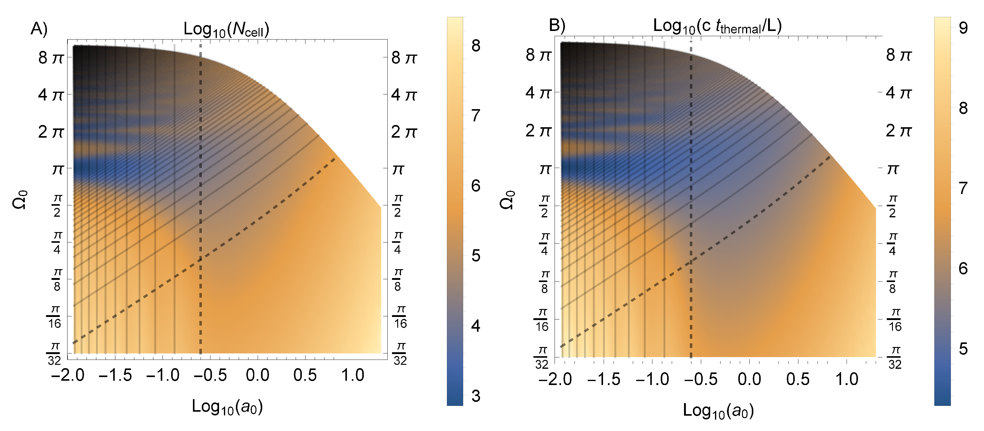
Of particular interest is the rate at which the probe approaches its final state. This is controlled by the relaxation rate which is given by the antisymmetric part of A, namely . The thermalization time is given by and the number of cells is given by . These quantities are shown in Figure A1 for a wide range of accelerations, , and probe gaps, with .
Figure A1.
The number of cells needed for convergence, , and the thermalization time are shown in (A,B) respectively. Please note that the axes are all on a logarithmic scale and we have fixed .
Figure A1.
The number of cells needed for convergence, , and the thermalization time are shown in (A,B) respectively. Please note that the axes are all on a logarithmic scale and we have fixed .

Of note is that at and the number of cells needed for thermalization is and the thermalization time is . For this is . For this is . It is worth noting how (and consequently ) depend on . At and we have the data shown in Figure A2, i.e., . By increasing the interaction strength, we can substantially decrease the thermalization time.
Figure A2.
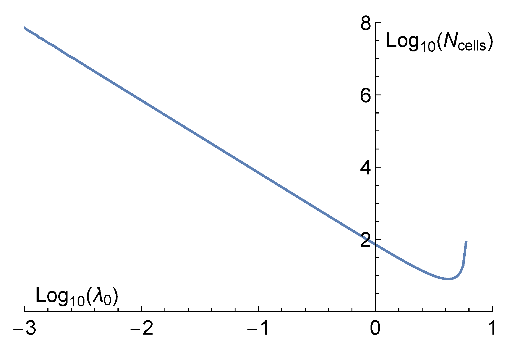
The number of cells needed for convergence is plotted against the dimensionless coupling strength . We have fixed here and . The line of best fit is or equivalently .
Figure A2.
The number of cells needed for convergence is plotted against the dimensionless coupling strength . We have fixed here and . The line of best fit is or equivalently .

Appendix C. Characterizing Temperature and Thermality of the Final Detector State
As we have discussed in the main text, we can efficiently compute the final covariance matrix of the detector, , after it has traveled through many cells. To characterize this state, we can write it in the standard form,
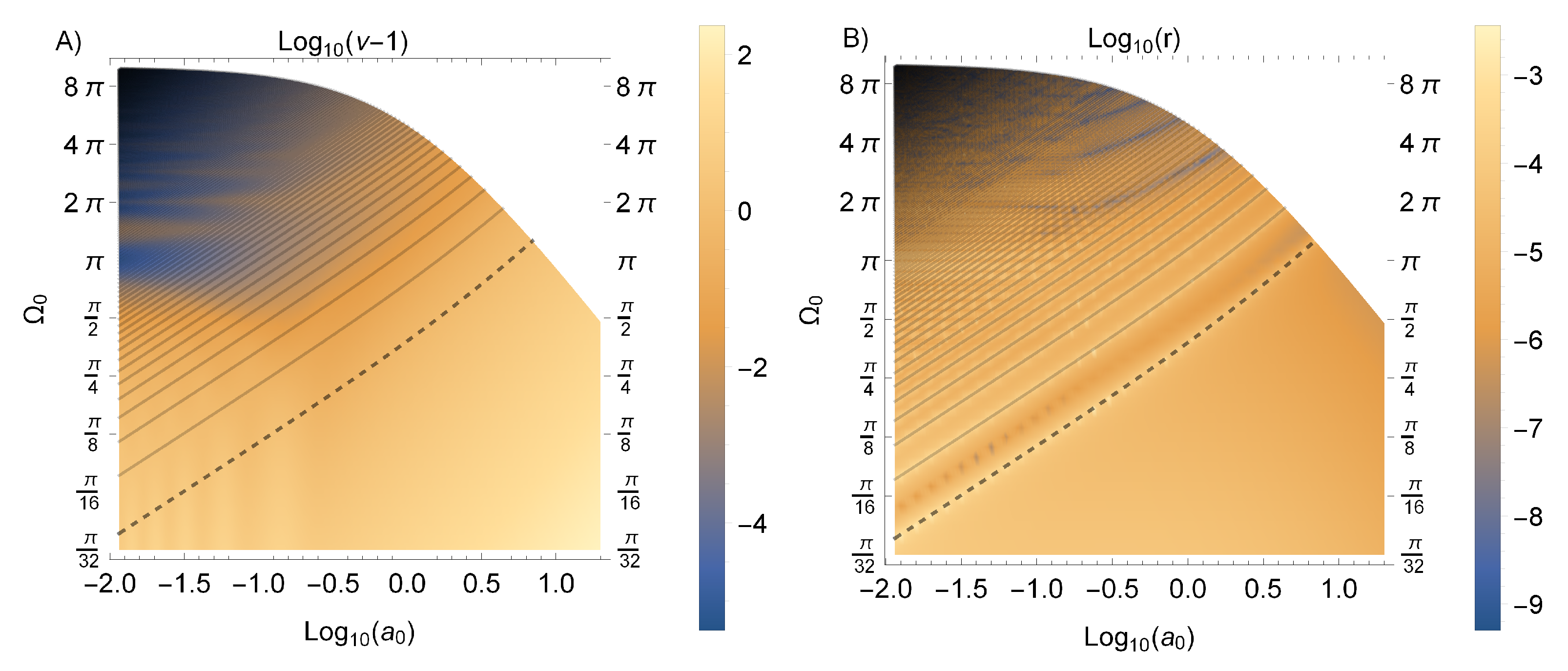
for some symplectic eigenvalue , squeezing parameter and angle where is the rotation matrix. The values of and r are shown in Figure A3 as functions of and . Please note that whereas . Thus, it appears that for the range of parameters we consider the final state of the detector is not very squeezed and is therefore approximately thermal. However, how can we quantify the degree to which the state is thermal?
Figure A3.
The symplectic eigenvalue and the squeezing parameter, r, of the final probe state are shown in (A,B) respectively. Please note that the axes are all on a logarithmic scale and we have fixed .
Figure A3.
The symplectic eigenvalue and the squeezing parameter, r, of the final probe state are shown in (A,B) respectively. Please note that the axes are all on a logarithmic scale and we have fixed .

In this section, we will establish that this state is in fact approximately thermal by showing that r is “small” in several different ways. Moreover, we will also explain the interesting band-like structure which appears in the plot of the squeezing parameter.
Appendix C.1. Thermality Criteria
Let us first consider the method of assessing thermality mentioned in the main text, and originally introduced in [28]. Specifically, we quantify how the energy needed to build the state from the vacuum is divided between the energy spent on squeezing and the energy spent on heating it to the corresponding unsqueezed thermal state. Concretely, the ratio of these energies is given by the following expression,
where is the average energy of a generic squeezed thermal state. Please note that the ground state (with and ) has (by convention) zero energy. We can use as a thermality criterion: if then the state’s squeezing energy is much less than its thermal energy. Please note that the test is harder to pass the nearer we are to the ground state, i.e., for fixed we have diverging as .
Figure A4A shows that in the regime where we see the Unruh effect. Thus, the state can be deemed very nearly thermal by this measure.
Figure A4.
The thermality measures and of the final probe state are shown in (A,B) respectively. Please note that the axes are all on a logarithmic scale and we have fixed .
Figure A4.
The thermality measures and of the final probe state are shown in (A,B) respectively. Please note that the axes are all on a logarithmic scale and we have fixed .

Another approach to characterizing the thermality of a Gaussian state is to generate a few different temperature estimates and demand their relative differences be small. A series of temperature estimates can be found by considering the relative populations of the detector’s energy levels. The probability of measuring a generic single-mode squeezed thermal state, , and finding n excitations is,
where and are the eigenvalues of . These expressions can be calculated straightforwardly by taking the overlap of a generic Gaussian Wigner function with the Fock state Wigner functions. From these we can compute the excitation de-excitation ratio (EDR) temperature estimates as,
We can declare that a state is reasonably thermal if many of its EDR temperature estimates between different energy levels all agree. For instance, we may consider the relative difference,
Expanding this relative difference for small r we find,
We can take to be an alternate thermality criterion to . Contrasting and we can see that is a harder test to pass, especially for near-ground states, i.e., for fixed , we have that diverges faster than as .
Figure A4B shows that over the range of parameters we consider. Despite being a harder test, we still find that the final probe state is approximately thermal (with respect to ), at least in the regime where we see the Unruh effect. Specifically, in the lower-right region of the plot we have .
In addition to and we have considered several other thermality measures, including comparing the EDR temperature estimates between different levels (e.g., versus ) as well as more information-theoretic measures (e.g., Hellinger and total variation distances). In each case these measures have indicated that the probe state is effectively indistinguishable from thermal in the regime where we see the Unruh effect.
Appendix C.2. Explaining the Bands
Looking at Figure A3B one may notice that there are bands of increased squeezing appearing in an ordered way. (The corresponding bands in Figure A4 are a consequence of this increased squeezing). We will now explain why these appear and why they are where they are.
The relevant quantity is the phase that the probe operators rotate through as the probe crosses one cavity, . Indeed, the bands lie on (or very near) the lines shown in Figure A3 and Figure A4. Please note that the line is dashed.
We can explain the occurrence of these bands as follows. Recall that the update map which we repeatedly apply is . Recall further that in the interaction picture, the update map for crossing the first cell is . Suppose that the effect of is to squeeze the state in some direction and then rotate it by an amount . The effect of would then be to squeeze the state in some direction and then rotate it by an amount .
First let us analyze the case where the effect of is a quarter-turn, . In this case, the second application of would immediately undo the squeezing done by the first application of . A similar phenomenon will happen for most values of . Over many applications of the state will have been squeezed in every direction more-or-less equally. The result in this case would be a minimally squeezed state.
The exception to this argument is when . In this case, the state is left unchanged by the rotation (note that squeezed states have a -rotational symmetry) such that it is squeezed in the same direction every time. This squeezing does not become infinite; however, as the dynamics also includes a relaxation rate. Thus, we expect a spike in the squeezing of the final state when .
Finally, we note that we have reason to believe that is small for all and . Recall that is the amount of rotation given by the interaction picture map . The interaction picture is designed to remove the free evolution/rotation of the system. Thus, only corresponds to the rotation induced in the probe by the interaction Hamiltonian. Thus, we expect spikes in the squeezing at which is just what we see.
Appendix D. Details on Mode Convergence
As we discussed in the main text, we truncate the number of cavity modes considered to make our computations tractable. In this section, we study the convergence of our results with the number of cavity modes considered.
We expect our scenario to have better convergence behavior than other previous studies on probes accelerating inside optical cavities (such as e.g., [28]) since in our setup the probe does not reach ultrarelativistic speeds with respect to the cavity walls. As such, the probe’s gap does not sweep across many cavity modes as it is blue/red-shifted () with respect to the lab frame. For instance, with and we have such that . Please note that even when maximally blue-shifted, the probe frequency is still below the frequency of the first cavity mode .
Another reason that one may worry that many cavity modes are required for convergence is that the probe suddenly couples/decouples from each cavity. Indeed, one can think of the probe having a top-hat switching function, . In general, one would expect that such a sudden change in the coupling would make high frequency cavity modes relevant. However, a key design feature of our setup regulates the suddenness of this switching. Specifically, the cavity’s Dirichlet boundary conditions enforce that the probe is effectively decoupled from the field at the time of this switching.
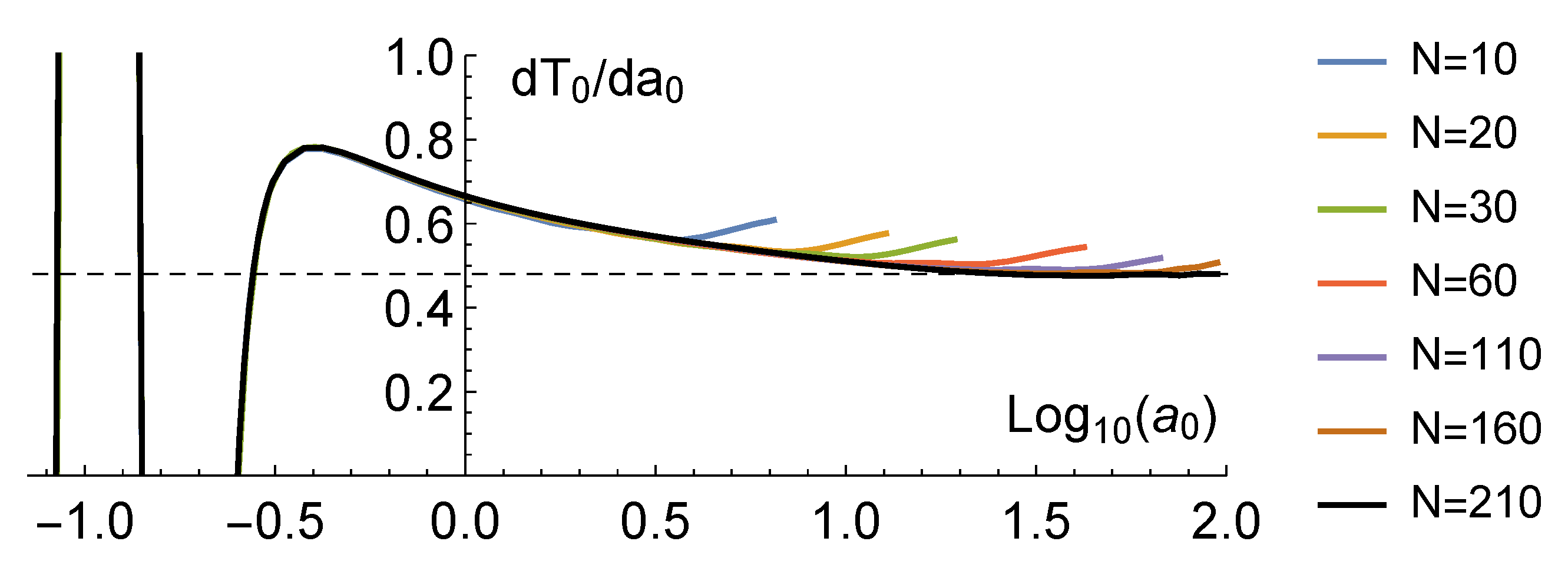
Taken together, these suggest that not too many cavity modes will be needed for convergence. Let us see how these expectations play out when we actually put them to the test. Figure A5 shows the line of Figure 1b of the main text converging as we increase the number of field modes, N, which we consider. Unsurprisingly, as the acceleration increases, we require more cavity modes for convergence. Figure A5 suggests that using modes is sufficient when and that using is sufficient when .
Figure A5.
Derivative of the probe’s final dimensionless temperature with respect to the acceleration as a function of on log-scale. The dimensionless probe gap, , and the dimensionless coupling strength, , are fixed. The black-dashed line is at . The colored lines show the values of which result from considering only N cavity modes where , 20, 30, 60, 110, 160, and 210. These lines split off from the rest one at a time in order from left to right.

References
- Fulling, S.A. Nonuniqueness of Canonical Field Quantization in Riemannian Space-Time. Phys. Rev. D 1973, 7, 2850. [Google Scholar] [CrossRef]
- Davies, P.C.W. Scalar particle production in Schwarzschild and Rindler metrics. J. Phys. A 1975, 8, 609. [Google Scholar] [CrossRef]
- Unruh, W.G. Notes on black-hole evaporation. Phys. Rev. D 1976, 14, 870. [Google Scholar] [CrossRef] [Green Version]
- Takagi, S. Vacuum Noise and Stress Induced by Uniform Acceleration: Hawking-Unruh Effect in Rindler Manifold of Arbitrary Dimension. Prog. Theor. Phys. Supp. 1986, 88, 1. [Google Scholar] [CrossRef]
- Crispino, L.C.B.; Higuchi, A.; Matsas, G.E.A. The Unruh effect and its applications. Rev. Mod. Phys. 2008, 80, 787. [Google Scholar] [CrossRef] [Green Version]
- Turner, M.S. Could primordial black holes be the source of the cosmic ray antiprotons? Nature 1982, 297, 379. [Google Scholar] [CrossRef]
- Hawking, S.W. Black hole explosions? Nature 1974, 248, 30. [Google Scholar] [CrossRef]
- Davies, P.C.W. Quantum vacuum noise in physics and cosmology. Chaos 2001, 11, 539. [Google Scholar] [CrossRef]
- Alsing, P.M.; Dowling, J.P.; Milburn, G.J. Ion trap simulations of quantum fields in an expanding universe. Phys. Rev. Lett. 2005, 94, 220401. [Google Scholar] [CrossRef] [Green Version]
- Gibbons, G.W.; Shellard, E.P.S. Tales of Singularities. Science 2002, 295, 1476. [Google Scholar] [CrossRef]
- Vanzella, D.A.T.; Matsas, G.E.A. Decay of accelerated protons and the existence of the fulling-davies-unruh effect. Phys. Rev. Lett. 2001, 87, 151301. [Google Scholar] [CrossRef] [Green Version]
- Taubes, G. String Theorists Find a Rosetta Stone. Science 1999, 285, 512. [Google Scholar] [CrossRef]
- Hossain, G.M.; Sardar, G. Is there unruh effect in polymer quantization? Class. Quantum Gravity 2016, 33, 245016. [Google Scholar] [CrossRef] [Green Version]
- Rovelli, C. LQG predicts the Unruh Effect. Comment to the paper “Absence of Unruh effect in polymer quantization” by Hossain and Sardar. arXiv 2014, arXiv:1412.7827. [Google Scholar]
- Martín-Martínez, E.; Fuentes, I.; Mann, R.B. Using berry’s phase to detect the unruh effect at lower accelerations. Phys. Rev. Lett. 2011, 107, 131301. [Google Scholar] [CrossRef] [PubMed] [Green Version]
- Chen, P.; Tajima, T. Testing unruh radiation with ultraintense lasers. Phys. Rev. Lett. 1999, 83, 256. [Google Scholar] [CrossRef] [Green Version]
- Cozzella, G.; Landulfo, A.G.S.; Matsas, G.E.A.; Vanzella, D.A.T. Proposal for observing the unruh effect using classical electrodynamics. Phys. Rev. Lett. 2017, 118, 161102. [Google Scholar] [CrossRef] [Green Version]
- Unruh, W.G. Experimental black-hole evaporation? Phys. Rev. Lett. 1981, 46, 1351. [Google Scholar] [CrossRef]
- Garay, L.J.; Anglin, J.R.; Cirac, J.I.; Zoller, P. Sonic analog of gravitational black holes in bose-einstein condensates. Phys. Rev. Lett. 2000, 85, 4643. [Google Scholar] [CrossRef] [Green Version]
- Hu, J.; Feng, L.; Zhang, Z.; Chin, C. Quantum simulation of unruh radiation. Nat. Phys. 2019, 15, 785. [Google Scholar] [CrossRef]
- Steinhauer, J. Observation of quantum hawking radiation and its entanglement in an analogue black hole. Nat. Phys. 2016, 12, 959–965. [Google Scholar] [CrossRef] [Green Version]
- Philbin, T.G.; Kuklewicz, C.; Robertson, S.; Hill, S.; König, F.; Leonhardt, U. Fiber-optical analog of the event horizon. Science 2008, 319, 1367. [Google Scholar] [CrossRef] [Green Version]
- Leonhardt, U. A laboratory analogue of the event horizon using slow light in an atomic medium. Nature 2002, 415, 406. [Google Scholar] [CrossRef] [Green Version]
- Nation, P.D.; Blencowe, M.P.; Rimberg, A.J.; Buks, E. Analogue hawking radiation in a dc-squid array transmission line. Phys. Rev. Lett. 2009, 103, 087004. [Google Scholar] [CrossRef] [Green Version]
- Alsing, P.; Dowling, J.; Milburn, G. The unruh effect in an ion trap: An analogy. arXiv 2004, arXiv:0411096. [Google Scholar]
- Horstmann, B.; Reznik, B.; Fagnocchi, S.; Cirac, J.I. Hawking radiation from an acoustic black hole on an ion ring. Phys. Rev. Lett. 2010, 104, 250403. [Google Scholar] [CrossRef] [Green Version]
- Carballo-Rubio, R.; Garay, L.J.; Martín-Martínez, E.; de Ramón, J. Unruh effect without thermality. Phys. Rev. Lett. 2019, 123, 041601. [Google Scholar] [CrossRef]
- Brenna, W.G.; Brown, E.G.; Mann, R.B.; Martín-Martínez, E. Universality and thermalization in the unruh effect. Phys. Rev. D 2013, 88, 064031. [Google Scholar] [CrossRef] [Green Version]
- Rad, N.; Singleton, D. A test of the circular unruh effect using atomic electrons. Eur. Phys. J. D 2012, 66, 258. [Google Scholar] [CrossRef] [Green Version]
- Bell, J.; Leinaas, J. Electrons as accelerated thermometers. Nucl. Phys. B 1983, 212, 131. [Google Scholar] [CrossRef] [Green Version]
- Bell, J.; Leinaas, J. The unruh effect and quantum fluctuations of electrons in storage rings. Nucl. Phys. B 1987, 284, 488. [Google Scholar] [CrossRef] [Green Version]
- Rogers, J. Detector for the temperaturelike effect of acceleration. Phys. Rev. Lett. 1988, 61, 2113. [Google Scholar] [CrossRef]
- Jin, Y.; Hu, J.; Yu, H. Spontaneous excitation of a circularly accelerated atom coupled to electromagnetic vacuum fluctuations. Ann. Phys. 2014, 344, 97. [Google Scholar] [CrossRef]
- Levin, O.; Peleg, Y.; Peres, A. Unruh effect for circular motion in a cavity. J. Phys. Math. Gen. 1993, 26, 3001. [Google Scholar] [CrossRef]
- Unruh, W. Acceleration radiation for orbiting electrons. Phys. Rep. 1998, 307, 163. [Google Scholar] [CrossRef] [Green Version]
- Biermann, S.; Erne, S.; Gooding, C.; Louko, J.; Schmiedmayer, J.; Unruh, W.G.; Weinfurtner, S. Unruh and analogue unruh temperatures for circular motion in 3 + 1 and 2 + 1 dimensions. Phys. Rev. D 2020, 102, 085006. [Google Scholar] [CrossRef]
- Lopp, R.; Martín-Martínez, E.; Page, D.N. Relativity and quantum optics: Accelerated atoms in optical cavities. Class. Quantum Gravity 2018, 35, 224001. [Google Scholar] [CrossRef] [Green Version]
- De Witt, B.S. Quantum gravity: The new synthesis. In General Relativity: An Einstein Centenary Survey; Cambridge University Press: Cambridge, UK, 1980; pp. 680–745. [Google Scholar]
- Cohen-Tannoudji, C.; Dupont-Roc, J.; Grynberg, G. Photons and Atoms: Introduction to Quantum Electrodynamics; Wiley: Hoboken, NJ, USA, 1989. [Google Scholar]
- Scully, M.O.; Zubairy, M.S. Quantum Optics; Cambridge University Press: Cambridge, UK, 1997. [Google Scholar] [CrossRef]
- Martín-Martínez, E.; Rodriguez-Lopez, P. Relativistic quantum optics: The relativistic invariance of the light-matter interaction models. Phys. Rev. D 2018, 97, 105026. [Google Scholar] [CrossRef] [Green Version]
- Lopp, R.; Martín-Martínez, E. Quantum delocalization, gauge and quantum optics: The light-matter interaction in relativistic quantum information. arXiv 2020, arXiv:2008.12785. [Google Scholar]
- Grimmer, D. Interpolated collision model formalism. arXiv 2020, arXiv:2009.10472. [Google Scholar]
- Grimmer, D.; Layden, D.; Mann, R.B.; Martín-Martínez, E. Open dynamics under rapid repeated interaction. Phys. Rev. A 2016, 94, 032126. [Google Scholar] [CrossRef] [Green Version]
- Grimmer, D.; Mann, R.B.; Martín-Martínez, E. Purification in rapid-repeated-interaction systems. Phys. Rev. A 2017, 95, 042114. [Google Scholar] [CrossRef] [Green Version]
- Giovannetti, V.; Palma, G.M. Master equations for correlated quantum channels. Phys. Rev. Lett. 2012, 108, 040401. [Google Scholar] [CrossRef] [PubMed] [Green Version]
- Caves, C.M.; Milburn, G.J. Quantum-mechanical model for continuous position measurements. Phys. Rev. A 1987, 36, 5543. [Google Scholar] [CrossRef] [Green Version]
- Altamirano, N.; Corona-Ugalde, P.; Mann, R.B.; Zych, M. Unitarity, feedback, interactions—Dynamics emergent from repeated measurements. New J. Phys. 2017, 19, 013035. [Google Scholar] [CrossRef] [Green Version]
- Lorenzo, S.; McCloskey, R.; Ciccarello, F.; Paternostro, M.; Palma, G.M. Landauer’s principle in multipartite open quantum system dynamics. Phys. Rev. Lett. 2015, 115, 120403. [Google Scholar] [CrossRef]
- Daryanoosh, S.; Baragiola, B.Q.; Guff, T.; Gilchrist, A. Quantum master equations for entangled qubit environments. Phys. Rev. A 2018, 98, 062104. [Google Scholar] [CrossRef] [Green Version]
- Cusumano, S.; Mari, A.; Giovannetti, V. Interferometric modulation of quantum cascade interactions. Phys. Rev. A 2018, 97, 053811. [Google Scholar] [CrossRef] [Green Version]
- Strasberg, P.; Schaller, G.; Brandes, T.; Esposito, M. Quantum and information thermodynamics: A unifying framework based on repeated interactions. Phys. Rev. X 2017, 7, 021003. [Google Scholar] [CrossRef] [Green Version]
- Lorenzo, S.; Ciccarello, F.; Palma, G.M. Composite quantum collision models. Phys. Rev. A 2017, 96, 032107. [Google Scholar] [CrossRef] [Green Version]
- Cusumano, S.; Mari, A.; Giovannetti, V. Interferometric quantum cascade systems. Phys. Rev. A 2017, 95, 053838. [Google Scholar] [CrossRef] [Green Version]
- Giovannetti, V.; Palma, G.M. Master equation for cascade quantum channels: A collisional approach. J. Phys. At. Mol. Opt. Phys. 2012, 45, 154003. [Google Scholar] [CrossRef]
- Attal, S.; Joye, A. Weak coupling and continuous limits for repeated quantum interactions. J. Stat. Phys. 2007, 126, 1241. [Google Scholar] [CrossRef] [Green Version]
- Bruneau, L.; Joye, A.; Merkli, M. Repeated interactions in open quantum systems. J. Math. Phys. 2014, 55, 075204. [Google Scholar] [CrossRef] [Green Version]
- Adesso, G. Entanglement of gaussian states. arXiv 2007, arXiv:quant-ph/0702069. [Google Scholar]
- Weedbrook, C.; Pirandola, S.; García-Patrón, R.; Cerf, N.J.; Ralph, T.C.; Shapiro, J.H.; Lloyd, S. Gaussian quantum information. Rev. Mod. Phys. 2012, 84, 621. [Google Scholar] [CrossRef]
- Lami, L.; Regula, B.; Wang, X.; Nichols, R.; Winter, A.; Adesso, G. Gaussian quantum resource theories. Phys. Rev. A 2018, 98, 022335. [Google Scholar] [CrossRef] [Green Version]
- Grimmer, D.; Brown, E.; Kempf, A.; Mann, R.B.; Martín-Martínez, E. A classification of open gaussian dynamics. J. Phys. A 2018, 51, 245301. [Google Scholar] [CrossRef] [Green Version]
- Grimmer, D.; Brown, E.; Kempf, A.; Mann, R.B.; Martín-Martínez, E. Gaussian ancillary bombardment. Phys. Rev. A 2018, 97, 052120. [Google Scholar] [CrossRef] [Green Version]
- Forn-Díaz, P.; Lamata, L.; Rico, E.; Kono, J.; Solano, E. Ultrastrong coupling regimes of light-matter interaction. Phys. Rev. A 2019, 91, 025005. [Google Scholar] [CrossRef] [Green Version]
- Smith, A.R.H.; Ahmadi, M. Quantum clocks observe classical and quantum time dilation. Nat. Comm. 2019, 11, 5360. [Google Scholar] [CrossRef] [PubMed]
- Unruh, W.G.; Wald, R.M. What happens when an accelerating observer detects a rindler particle. Phys. Rev. D 1984, 29, 1047. [Google Scholar] [CrossRef]
- Mourou, G.A.; Tajima, T.; Bulanov, S.V. Optics in the relativistic regime. Rev. Mod. Phys. 2006, 78, 309. [Google Scholar] [CrossRef] [Green Version]
- Kazantsev, A.P. The acceleration of atoms by light. In 30 Years of the Landau Institute—Selected Papers; World Scientific: Singapore, 1996; pp. 102–108. [Google Scholar] [CrossRef]
- Livingston, A.B. Physics Division Progress Report for Period Ending September 30, 1988; Oak Ridge National Lab.: Oak Ridge, TN, USA, 1989. [CrossRef] [Green Version]
Figure 1.
(a) Derivative of the probe’s final temperature with respect to the acceleration as a function of and the probe gap on log-scale. The dimensionless coupling strength is fixed at . The Unruh effect () is found in the lower-right portion of the figure. Black lines highlight relevant physical scales (see main text). (b) Cross-sections of as a function of for several detector gaps: (from top to bottom at ) showing independence of in the Unruh effect regime. The black-dashed line is at .

Figure 2.
A schematic drawing of one possible implementation of our experimental proposal. Voltages at the cavity walls accelerate and decelerate the probe.
Figure 2.
A schematic drawing of one possible implementation of our experimental proposal. Voltages at the cavity walls accelerate and decelerate the probe.


Table 1.
Our proposed setup with , and realized at two different scales, (tabletop) and (LIGO-sized). estimates the lab-time needed for the probe to thermalize. is the number of cells crossed in this time. Note these can be substantially decreased by increasing . See Appendix B for details on and .
Table 1.
Our proposed setup with , and realized at two different scales, (tabletop) and (LIGO-sized). estimates the lab-time needed for the probe to thermalize. is the number of cells crossed in this time. Note these can be substantially decreased by increasing . See Appendix B for details on and .
| Tabletop | LIGO-Sized | |
|---|---|---|
| L | ||
| a | ||
| 0.051 | 0.051 | |
| T | ||
Publisher’s Note: MDPI stays neutral with regard to jurisdictional claims in published maps and institutional affiliations. |
© 2021 by the authors. Licensee MDPI, Basel, Switzerland. This article is an open access article distributed under the terms and conditions of the Creative Commons Attribution (CC BY) license (https://creativecommons.org/licenses/by/4.0/).
Share and Cite
MDPI and ACS Style
Vriend, S.; Grimmer, D.; Martín-Martínez, E. The Unruh Effect in Slow Motion. Symmetry 2021, 13, 1977. https://0-doi-org.brum.beds.ac.uk/10.3390/sym13111977
AMA Style
Vriend S, Grimmer D, Martín-Martínez E. The Unruh Effect in Slow Motion. Symmetry. 2021; 13(11):1977. https://0-doi-org.brum.beds.ac.uk/10.3390/sym13111977
Chicago/Turabian StyleVriend, Silas, Daniel Grimmer, and Eduardo Martín-Martínez. 2021. "The Unruh Effect in Slow Motion" Symmetry 13, no. 11: 1977. https://0-doi-org.brum.beds.ac.uk/10.3390/sym13111977
Note that from the first issue of 2016, this journal uses article numbers instead of page numbers. See further details here.