Article

Analysis for Xgamma Parameters of Life under Type-II Adaptive Progressively Hybrid Censoring with Applications in Engineering and Chemistry

by
Ahmed Elshahhat
1,* and
Berihan R. Elemary
2,3
1
Faculty of Technology and Development, Zagazig University, Zagazig 44519, Egypt
2
Department of Applied Mathematical and Actuarial Statistics, Faculty of Commerce, Damietta University, Damietta 34511, Egypt
3
Faculty of Business Administration, NUB-Nahda University, Beni Suef 62513, Egypt
*
Author to whom correspondence should be addressed.
Submission received: 29 September 2021 / Revised: 28 October 2021 / Accepted: 3 November 2021 / Published: 7 November 2021

Abstract

:
Censoring mechanisms are widely used in various life tests, such as medicine, engineering, biology, etc., as they save (overall) test time and cost. In this context, we consider the problem of estimating the unknown xgamma parameter and some survival characteristics, such as reliability and failure rate functions in the presence of adaptive type-II progressive hybrid censored data. For this purpose, the maximum likelihood and Bayesian inferential approaches are used. Using the observed Fisher information under s-normal approximation, different asymptotic confidence intervals for any function of the unknown parameter were constructed. Using the gamma flexible prior, Bayes estimators against the squared-error loss were developed. Two procedures of Bayesian approximations—Lindley’s approximation and Metropolis–Hastings algorithm—were used to carry out the Bayes estimates and to construct the associated credible intervals. An extensive simulation study was implemented to compare the performance of the different methods. To validate the proposed methodologies of inference—two practical studies using datasets that form engineering and chemical fields are discussed.

1. Introduction

The gamma distribution is one of the most popular models used for analyzing constant and non-constant failure rate data. It includes the exponential, Erlang, and chi-square distributions as special cases. In recent years, using exponential and/or gamma as the parent distribution (among others), several new models have been developed to provide richness that makes them accurate and suitable to fit complex datasets. New statistical models, created based on a finite mixture of probability distributions, played a vital role in modeling the real-life phenomenon. Further, finite mixture densities have been widely used to model various data, for example, see [1,2]. However, gamma distribution does not exhibit a bathtub or upside-down bathtub shaped hazard rate function and, thus, it cannot be used to model the complex lifetime of a system.
For this reason, Reference [3] proposed a new one-parameter xgamma distribution, denoted by XGD ( δ ) , as a special finite mixture of exponential and gamma distributions. They derived various mathematical, structural, and survival properties, with inference to the XGD. Moreover, they showed that the XGD was useful in modeling the dataset with a monotone failure rate, and that it had applicability in analyzing lifetime data.
Suppose that the lifetime random variable X of an experimental unit(s) follows XGD ( δ ) , then, the probability density function (PDF) f ( · ) and cumulative distribution function (CDF) F ( · ) of X, are given, respectively, by
f ( x ; δ ) = δ 2 1 + δ 1 + 1 2 δ x 2 e δ x , x > 0 , δ > 0 ,
and
F ( x ; δ ) = 1 1 + δ 1 + x + 1 2 δ x 2 1 + δ e δ x , x > 0 , δ > 0 ,
where δ is the scale parameter. The reliability characteristics of any lifetime model are the main features for evaluating the capacity of any electronic system that a reliability practitioner frequently uses. Therefore, some survival parameters of the XGD are also investigated as unknown parameters; reliability function (RF) R ( · ) and failure rate function (FRF) h ( · ) at mission time t are given, respectively, by
R ( t ; δ ) = 1 + δ 1 + t + 1 2 δ t 2 1 + δ e δ t , t > 0 , δ > 0 ,
and
h ( t ; δ ) = 1 + 1 2 δ t 2 1 + δ 1 + t + 1 2 δ t 2 δ 2 , t > 0 , δ > 0 ,
Moreover, Reference [3] indicates that the XGD belongs to the exponential family of distributions and it has more flexibility than the exponential distribution. Reference [4] studied the estimation procedures of the XGD parameter and some related important survival characteristics under type-II progressively censoring (PCS-T2). Furthermore, they showed that the xgamma random variates are stochastically larger than that of the exponential and Lindley distributions. Reference [5] discussed the estimating problem of the parameter and reliability characteristics of XGD under hybrid type-II censored data. Recently, Reference [6] derived both classical and Bayes estimates of some parameters of life for XGD under complete sampling.
The adaptive type-II progressive hybrid censoring scheme (APHCS-T2), introduced by [7], saves the total time test and increases the efficiency of statistical inference. It can be described in the context of a life testing experiment as follows: suppose that n identical units are placed on the test at time zero; m ( 1 m < n ) is the pre-fixed number of failures and the experimental time is allowed to run over time T, which is an ideal total test. In this case, the progressive censoring R i , i = 1 , 2 , , m , is provided, but the values of some of R i may change accordingly during the experiment. If X ( m ) < T , the experiment proceeds with R i s and stops at X ( m ) . In this situation, APHCS-T2 degenerates into usual PCS-T2 and the experiment stops at the time of observe m-th failure. Otherwise, if X ( m ) does not occur before time T, i.e., X ( d ) < T < X ( d + 1 ) , where ( d + 1 ) < m and X ( d ) is the d-th failure, occur before time T, then no items will be withdrawn from the experiment by setting R i = 0 for i = d + 1 , , m 1 , and the experiment stops at the time of the m-th failure occurring, and all remaining surviving items are removed, i.e., R m = n m i = 1 d R i . The main advantage of APHCS-T2 is it enables us to get the effective number of failures m and assures that the total test time will not be too far away from the pre-specified time T.
If n units put on a life test are from a continuous population with CDF F ( x ) and PDF f ( x ) , and m effective number of failures have been observed, hence, the joint PDF for the ordered failure times of APHCS-T2 out of the experiment x ( i ) , i = 1 , 2 , , m , where θ ̲ is parameter vector, is given by
L θ ̲ d = C d Π m i = 1 f x ( i ) ; θ ̲ Π d i = 1 1 F x ( i ) ; θ ̲ R i 1 F x ( m ) ; θ ̲ R m * ,
where C d = Π m i = 1 n i + 1 j = 1 max i 1 , d R j and R m * = n m i = 1 d R i .
Several works based on APHCS-T2 have investigated the problem of estimating the unknown parameters of different lifetime models, e.g., see [8,9,10,11,12,13,14,15,16,17,18,19,20,21,22].
To the best of our knowledge, we have not come across any work related to the estimation of distribution parameters and/or reliability characteristics of the XGD under adaptive progressive censoring. Thus, by demonstrating that the XGD may be used as a survival model utilizing APHCS-T2, the purpose of this study is to close this gap. Thus, our objectives in this study are: first, to drive both point and interval estimators of the unknown parameter and survival characteristics, the XGD using both maximum likelihood and Bayesian approaches in the present data collected under the APHCS-T2 life test. Using gamma density prior under the squared-error loss (SEL) function, the Bayes estimators (BEs) for the unknown parameter and the survival characteristics are obtained. When the informative prior density is taken into account, an approach used to determine the hyperparameter values is proposed. Second, the proposed estimators cannot be obtained in explicit expressions, we apply some numerical procedures to evaluate them, such as the Newton–Raphson (N–R) iterative method, Lindley’s approximation, and Metropolis–Hastings (M–H) algorithm. Presently, Bayesian statistics that are developed based on Markov chain Monte Carlo (MCMC) techniques are widely used in many fields. Using normal approximation of the MLE (NA) and of the log-transformed MLE (NL), approximate confidence intervals (ACIs) for the unknown parameters, and any function of them, are constructed. Moreover, using MCMC simulated samples, two-sided BCI/HPD credible intervals are also constructed. Extensive numerical comparisons have been made to compare the performance of the classical and Bayesian estimates. The point estimates have been compared in terms of their estimated root mean squared errors (RMSEs) and relative absolute biases (RABs). Further, the interval estimates have been compared in terms of their average confidence widths (ACWs). Lastly, two datasets from industrial and chemical fields are analyzed to illustrate our proposed estimators.
The rest of the paper is organized as follows: maximum likelihood and Bayesian inferential procedures of the unknown parameter and the reliability characteristics are provided in Section 2 and Section 3, respectively. In Section 4, asymptotic and credible intervals are constructed. Monte Carlo simulation results are presented in Section 5. Two practical examples using real datasets are analyzed and investigated in Section 6. Finally, some concluding remarks are provided in Section 7.

2. Likelihood Inference

Suppose X ( 1 ) < · · · < X ( d ) < T < X ( d + 1 ) < · · · < X ( m ) , where ( 1 d < m < n ), is an APHCS-T2 sample drawn from an xgamma population whose PDF (1) and CDF (2), with their respective removal patterns are R 1 , , R d , 0 , , 0 , n m i = 1 d R i . Henceforward, we will use X i instead of X i : m : n . Substituting (1) and (2) into (5), the likelihood function (5) can be written up to proportional as
L δ x ̲ δ 2 m e δ ψ 1 + δ Q Π m i = 1 1 + 1 2 δ x i 2 × Π d i = 1 1 + δ 1 + x i + 1 2 δ x i 2 R i 1 + δ 1 + x m + 1 2 δ x m 2 R m * ,
where ψ ( x ) = x m R m * + i = 1 m x i + i = 1 d x i R i and Q = m + R m * + i = 1 d R i .
The corresponding log-likelihood function, ( · ) log L ( · ) , of (6) becomes
δ x ̲ ( 2 m ) log ( δ ) δ ψ ( x ) Q log ( 1 + δ ) + i = 1 m log 1 + δ x i 2 / 2 + i = 1 d R i log ξ x i ; δ + R m * log ξ x m ; δ ,
where ξ ( x i ; δ ) = 1 + δ 1 + x i + 1 2 δ x i 2 and ξ ( x m ; δ ) = 1 + δ 1 + x m + 1 2 δ x m 2 .
From (7), the MLE δ ^ of δ can be obtained by solving of the following likelihood equation
2 m δ ^ ψ x δ ^ Q 1 + δ ^ + i = 1 m x i 2 / 2 1 + δ ^ x i 2 / 2 + i = 1 d R i ξ ^ x i ; δ ^ ξ ^ x i ; δ ^ + R m * ξ ^ x m ; δ ^ ξ ^ x m ; δ ^ = 0 ,
where ξ ( · ) is the first-derivative with respect to δ such as ξ ( x i ; δ ) = 1 + x i 1 + δ x i and ξ ( x m ; δ ) = 1 + x m 1 + δ x m .
It is clear that, from (8), a closed-form solution of δ ^ does not exist and cannot be obtained analytically. Thus, one may use any suitable numerical procedure, such as the N–R iterative method to obtain the desired MLE δ ^ for any given values of n, m, T and ( x i , R i ) , i = 1 , 2 , , m . Once the estimate of δ ^ is obtained, then the associated MLEs of the parameters of life, R ( · ) and h ( · ) (for t > 0 ), can be easily derived via replacing δ by δ ^ , respectively, as
R ^ ( t ; δ ^ ) = 1 + δ ^ 1 + t + 1 2 δ ^ t 2 1 + δ ^ e δ ^ t , t > 0 ,
and
h ^ ( t ; δ ^ ) = 1 + 1 2 δ ^ t 2 1 + δ ^ 1 + t + 1 2 δ ^ t 2 δ ^ 2 , t > 0 .

3. Bayes Procedure

In this section, the Bayes estimators of the unknown parameters δ , R ( · ) and h ( · ) are developed under the SEL function, l S ( · ) , which is defined as
l S η , η ˜ = η ˜ η 2 .
Using (9), the Bayes estimator η ˜ ( δ ) (say) of the unknown parameter or any function of δ , η ( δ ) (say), is given by the posterior mean of η ( δ ) . However, any other loss function can be easily incorporated. It is known that the family of gamma distributions is flexible enough to cover a large variety of prior beliefs of the experimenter, see [23]. Therefore, we assume that the unknown parameter δ is stochastically independently distributed with conjugate gamma prior, as
π δ δ a 1 exp b δ , a , b , δ > 0 .
Combining (10) with (6) and substituting in the continuous Bayes’ theorem, the posterior PDF of δ becomes
π δ x ̲ δ 2 m + a 1 exp ( δ ( b + ψ ) ) 1 + δ Q Π m i = 1 1 + 1 2 δ x i 2 Π d i = 1 ξ ( x i ; δ ) R i ξ ( x m ; δ ) R m * ,
where C is the normalizing constant of (11) and is given by C = 0 π δ x ̲ d δ .
Hence, using (11), the Bayes estimate of any parameter of life η δ = δ , R ( t ) , h ( t ) (say) against the SEL function is given by
η ˜ ( δ ) = E δ η ( δ ) x ̲ = 0 η ( δ ) · π δ x ̲ d δ 0 π δ x ̲ d δ ·
It is clear that the posterior PDF (11) is not easily tractable due to its implicit mathematical expression, so the BEs (12) cannot be developed in a closed-form. To overcome this problem, two approximation techniques, namely: Lindley and MCMC procedures, are used.

3.1. Lindley’s Approximation

Reference [24] suggested procedure is to approximate the desired Bayes estimator by reducing the posterior ratio to finite values. According to this procedure, the approximated value η ^ ( δ ) of η ( δ ) as in (12) for any function of δ for a sufficiently large sample size n is given by
η ^ ( δ ) = η ( δ ) + 1 2 η 2 ( δ ) + 2 η 1 ( δ ) ρ σ 2 + 1 2 η 1 ( δ ) L 3 σ 4 ,
where η i ( δ ) = i η ( δ ) / δ i , i = 1 , 2 ; σ 2 = ( L 2 ) 1 ; σ 4 = ( L 2 ) 2 ; L i = i ( · ) / δ i , i = 2 , 3 ; and ρ = log π ( · ) / δ . All terms of (13) are evaluated at δ = δ ^ .
Now, to approximate the Bayes estimators using (13), the following quantities must be obtained as
L 2 = 2 m δ 2 + Q 1 + δ 2 i = 1 m x i 4 / 4 1 + δ x i 2 / 2 2 + i = 1 d R i ξ i 2 ξ i ξ i ξ i 2 + R m * ξ m 2 ξ m ξ m ξ m 2 ,
L 3 = 4 m δ 3 2 Q 1 + δ 3 + i = 1 m x i 4 / 2 1 + δ x i 2 / 2 3 + i = 1 d R i ξ i 4 ξ i 2 ξ i ξ i ξ i ξ i 2 ξ i ξ i ξ i ξ i ξ i 2 + R m * ξ m 4 ξ m 2 ξ m ξ m ξ m ξ m 2 ξ m ξ m ξ m ξ m ξ m 2 ,
and
ρ = ( a 1 ) / δ b ,
where ξ ( · ) and ξ ( · ) are the second- and third-derivatives, with respect to δ as ξ i = ξ ( x i ; δ ) = x i 2 , ξ m = ξ ( x m ; δ ) = x m 2 , ξ i = ξ ( x i ; δ ) = 0 and ξ m = ξ ( x m ; δ ) = 0 . The approximate BEs η ^ ( δ ) of η ( δ ) , using the Lindley’s approximation method, can be easily obtained. Unfortunately, in literature, we have not yet come up with a method that can be used to construct the associate credible intervals of the unknown parameters η ( δ ) using Lindley’s procedure. In view of this, we propose to use the M–H algorithm in order to generate MCMC samples from the posterior distribution and then to compute the Bayes estimators and also to construct the associated credible intervals.

3.2. M–H Algorithm

The M–H algorithm, a useful one of MCMC techniques, is used for generating random samples from the posterior distribution by an independent proposal distribution. However, from a practical point of view, this method provides a chain form of the Bayesian estimate, which is easy to apply in practice. One may refer to [25] and [26] for more applications related to this algorithm. To implement the M–H algorithm procedure, conduct the following steps for the sample generation process:
Step 1: Start with an initial guess δ ( 0 ) = δ ^ .
Step 2: Set j = 1 .
Step 3: Generate δ ( j ) from π ( δ ( j 1 ) | x ̲ ) with the normal proposal density distribution as
(a)
Obtain a candidate value δ * from N ( δ ( j 1 ) , Var ( δ ) ) .
(b)
Obtain a sample point u from uniform distribution U ( 0 , 1 ) .
(c)
Obtain δ ( j 1 ) , δ * = min π δ * x ̲ π δ ( j 1 ) x ̲ , 1 .
(d)
Set δ ( j ) = δ * if u ( · ) , otherwise set δ ( j ) = δ ( j 1 ) .
Step 4: Set j = j + 1 .
Step 5: Repeat steps 2–4 for a large N times to obtain δ ( j ) , j = 1 , 2 , , N .
Step 6: Using the outputs of Step 5, compute the parameters of life of XGD ( δ ) , such as R ( t ) and h ( t ) , for a distinct time t > 0 as
R ( j ) ( t ) = 1 + δ ( j ) 1 + t + 1 2 δ ( j ) t 2 1 + δ ( j ) e δ ( j ) t ,
and
h ( j ) ( t ) = 1 + 1 2 δ ( j ) t 2 1 + δ ( j ) 1 + t + 1 2 δ ( j ) t 2 δ ( j ) 2 ,
respectively.
To remove the affection of the initial guess and to guarantee the convergence of the sampler, the first simulated varieties, N 0 (say), usually discarded in the beginning of the analysis implementation (burn-in period). Hence, the selected MCMC samples η ( j ) δ = ( δ ( j ) , R ( j ) ( t ) , h ( j ) ( t ) ) for j = N 0 + 1 , , N can be used to develop the Bayesian inferences. However, the Bayes MCMC estimates of a parametric function η δ based on the SEL function are given by
η ˜ S δ = j = N 0 + 1 N η ( j ) ( δ ) N N 0 ·

3.3. Hyper-Parameter Value Selection

The elicitation procedure used to determine the hyperparameter value, when an informative prior of the density parameter is taken into account, is the main issue in Bayesian analysis. In the literature, this problem has been discussed by [27,28]. Moreover, the values of hyperparameters for the unknown parameters under interest are made by assuming two independent types of information, namely prior mean and prior variance of the unknown parameter of the model under consideration. In this regard, we propose the following steps to determine the values of hyperparameters a and b, based on past samples as
Step 1: Set the parameter value of δ .
Step 2: Set the complete sample size n.
Step 3: Draw a random sample of size n from XGD ( δ ) .
Step 4: Compute the MLE δ ^ of δ .
Step 5: Repeat Steps 2–4 B times to get δ ^ J , J = 1 , 2 , , B .
Step 6: Set the sample mean and sample variance of δ ^ J equal to the mean and variance of the gamma density prior, respectively, as
E ( δ ^ j ) E ( π ( δ ) ) 1 B J = 1 B δ ^ J = a b ,
and
Var ( δ ^ j ) Var ( π ( δ ) ) 1 B 1 J = 1 B δ ^ J B 1 J = 1 B δ ^ J 2 = a b 2 ,
where B is the number of samples generated from the distribution under consideration.
Step 7: Solve (15) and (16) simultaneously, the estimated hyperparameters a ˘ and b ˘ of a and b can be turn out directly by
a ˘ = 1 B J = 1 B δ ^ J 2 1 B 1 J = 1 B δ ^ J B 1 J = 1 B δ ^ J 2 and b ˘ 1 B J = 1 B δ ^ J 1 B 1 J = 1 B δ ^ J B 1 J = 1 B δ ^ J 2 ,
respectively.

4. Asymptotic and Credible Intervals

In this section, using NA and NL approximations of the MLE, the associated two-sided ACIs of the unknown parameter δ or any characteristic function, such as R ( · ) and h ( · ) , are constructed. In addition, the simulated MCMC varieties of these unknown parameters are used to construct the associated BCI and HPD credible intervals.

4.1. Asymptotic Confidence Intervals

The asymptotic normal distribution of the MLE is the most common method to obtain the confidence bounds. In our problem, the exact distribution of δ ^ cannot be obtained easily due to the MLE δ ^ as (8) has a nonlinear expression. Therefore, the observed Fisher information, I ( · ) , is used to develop the 100 ( 1 ε ) % ACI of δ by taking the negative expectation of the second-derivative (or Hessian matrix) of (7) as I ( δ ^ ) = L 2 , where L 2 is given in (14). Consequently, the approximate variance of the MLE δ ^ is given by
Var ^ ( δ ^ ) = I 1 ( δ ^ ) .
However, as referred to in Section 1, the XGD ( δ ) belongs to one-parameter exponential family of distributions. Therefore, the sampling distribution of ( δ δ ^ ) / Var ^ ( δ ^ ) can be easily approximated by a standard normal distribution, N ( 0 , 1 ) , see [29]. Then, using the concept of large sample theory based on the NA of the MLE δ ^ , the 100 ( 1 ε ) % two-sided ACI of δ is given by
δ ^ z ε / 2 Var ^ ( δ ^ ) ,
where z ε / 2 is the percentile of the standard normal distribution with right-tail probability ( ε / 2 ) -th. Since the characteristic parameters, such as R ( · ) and h ( · ) , denoted by φ ( δ ) (say), are continuous functions of δ , then using the approximate variance of the unknown parameter δ , the corresponding variance estimate of any function of δ can be approximated by
Var ^ ( φ ^ ( δ ^ ) ) = φ ( δ ) / δ 2 I 1 ( δ ) δ = δ ^ ,
where I 1 ( · ) is given by (18), see [30]. Similarly, based on the NA of the MLEs φ ^ ( δ ^ ) , the 100 ( 1 ε ) % two-sided ACIs for φ ^ ( δ ) can be obtained by
φ ^ ( δ ^ ) z ε / 2 Var ^ ( φ ^ ( δ ^ ) ) ,
where z ε / 2 is the percentile of the standard normal distribution with upper probability ( ε / 2 ) -th.
In some situations, the lower bound of standard ACI using normal approximation may take a negative value for a life distribution parameter. To overcome this drawback, one may replace the zero value instead of the negative value or using the NL in order to construct ACIs for the unknown parameters that take positive values, see [31]. Recently, the NL of the MLE was used by several authors, for example, see [32,33,34]. Hence, using the concept of the large sample, the 100 ( 1 ε ) % two-sided ACI based on the NL for the MLE of any function of η ( δ ) is given by
η ( δ ^ ) × exp z ε / 2 Var ^ ( η ( δ ^ ) ) η ( δ ^ ) ,
where η ( δ ^ ) = ( δ ^ , R ^ ( t ) , h ^ ( t ) ) and z ε / 2 is the percentile of the standard normal distribution with upper probability ( ε / 2 ) -th.

4.2. Credible Intervals

The interval based on posterior distribution is known as the Bayesian confidence interval and is called a credible interval. To construct the two-sided BCIs, the unknown model parameter δ and the survival characteristics R ( t ) and h ( t ) , order the simulated MCMC variates of η ( j ) ( δ ) = ( δ ( j ) , R ( j ) ( t ) , h ( j ) ( t ) ) for j = N 0 + 1 , , N as ( δ ( N 0 + 1 ) , , δ ( N ) ) , ( R ( N 0 + 1 ) ( t ) , , R ( N ) ( t ) ) and ( h ( N 0 + 1 ) ( t ) , , h ( N ) ( t ) ) . Hence, the 100 ( 1 ε ) % two-sided BCI for any function of η δ is given by
η N N 0 ε / 2 , η N N 0 1 ε / 2 ,
where η ( x ) ( y ) is an objective estimate located at the ordered point x y in the MCMC simulated variates after burn-in.
According to the method proposed by [35], using the ordered MCMC variates of η ( j ) δ for j = N 0 + 1 , , N , the 100 ( 1 ε ) % HPD credible interval for any function of δ as η ( δ ) can be constructed as
η j * , η j * + 1 ε N N 0 ,
where j * is chosen such that
η j * + [ 1 ε N N 0 ] η j * = min 1 j ε N N 0 η j + [ 1 ε N N 0 ] η j , j * = N 0 + 1 , , N .
Here, [ x ] denotes the largest integer less than or equal to x.

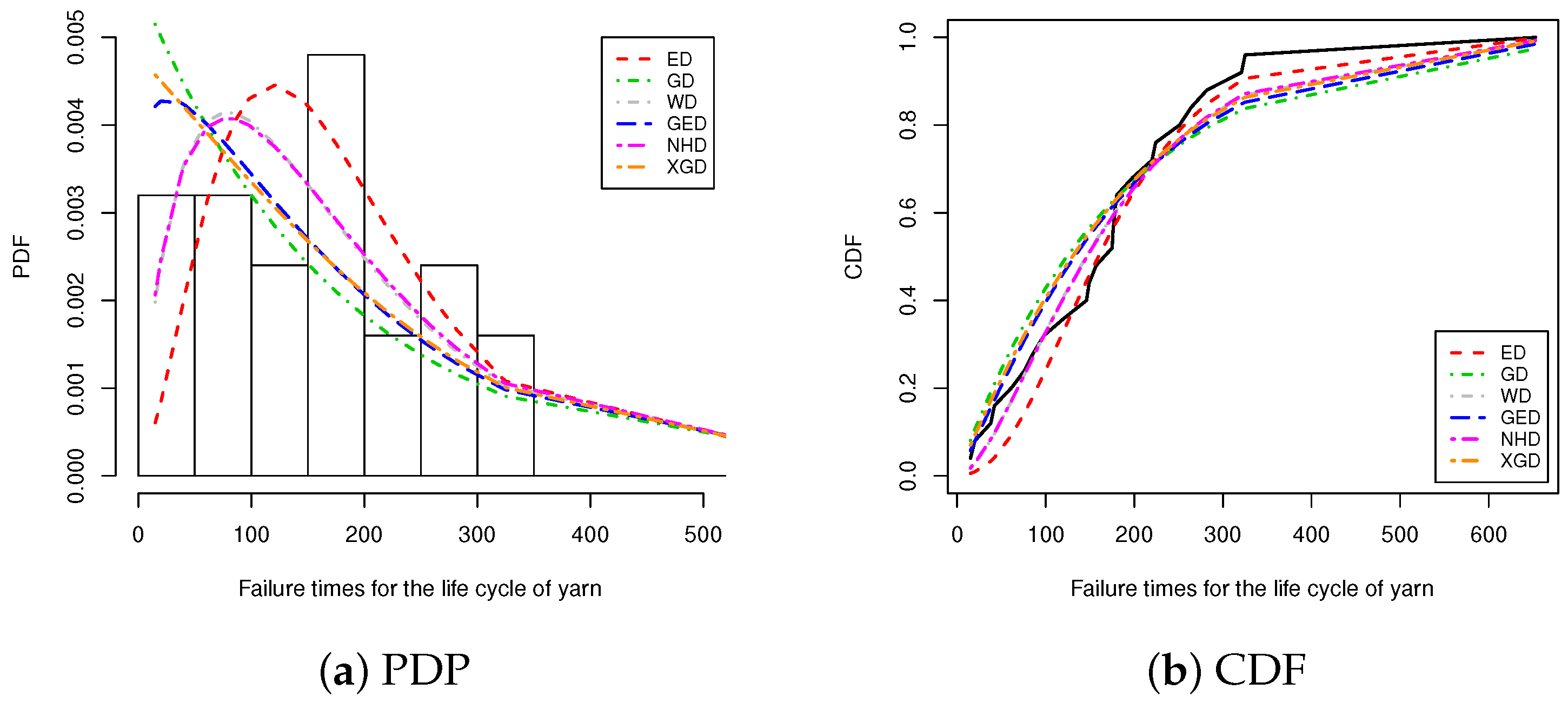
5. Monte Carlo Simulation

To examine the behavior of considered estimators of the model parameter, as well as associated reliability and hazard rate functions of XGD based on APHCS-T2, various Monte Carlo simulations are conducted by considering two different true values of the xgamma parameter as δ ( = 1 , 3 ) . Using the algorithm described in [7], a large number, 1000 of APHCS-T2 samples based on different combinations of n (number of total test units) and m (effective sample size) are generated from XGD ( δ ) .
For each setting, the MLEs and Bayes MCMC estimates of the unknown parameter δ and the reliability characteristics R ( t ) and h ( t ) are computed. Approximate Bayes computations are developed using both Lindley and M–H algorithm methods. Now, to generate APHCS-T2 samples from the XGD model, conduct the following steps:
Step 1: generate an ordinary PCS-T2 sample ( X i , R i ) , i = 1 , 2 , , m , by using the algorithm described by [36] as
(a)
Generate W independent observations of size m as W 1 , W 2 , , W m .
(b)
For given values of n, m, T and R i , i = 1 , 2 , , m , set V i = W i i + j = m i + 1 m R j 1 , for i = 1 , 2 , , m .
(c)
Set U i = 1 V m V m 1 V m i + 1 for i = 1 , 2 , , m . Hence, U i , i = 1 , 2 , , m is a PCS-T2 sample of size m from U ( 0 , 1 ) distribution.
(d)
Invert (2) for a given value of δ , i.e., X i = F 1 ( u i ; δ ) , i = 1 , 2 , , m , the PCS-T2 sample from XGD ( δ ) is carried out.
Step 2: Determine d-th failure, where X d < T < X d + 1 , and discard the remaining sample X d + 2 , , X m .
Step 3: Generate the first m d 1 order statistics from a truncated distribution f x 1 F x d + 1 with sample size n d j = 1 d R j 1 as X d + 2 , , X m .
This numerical comparison is performed based on different combinations of ( n , m , T ) , such as: n ( = 30 , 80 ) for each pre-determined time T ( = 1 , 3 ) . The test is terminated when the number of failed subjects achieves or exceeds a certain value m, where the percentage of failure information ( m / n ) is taken as 50 and 80%.
To assign values for the hyperparameters of the conjugate gamma prior (10), we propose using the procedure of past sample data described in Section 3.3. In view of this, we generated 1000 complete samples of a large size 50 (say) from the xgamma lifetime model as past samples when the plausible values of an unknown parameter δ were taken as 1 and 3. Consequently, the values of the hyperparameters a and b, which are plugged-in to the computation of the desired Bayes estimates, are taken as ( a , b ) = ( 98.295 , 97.046 ) and ( a , b ) = ( 77.136 , 25.384 ) for XGD ( 1 ) and XGD ( 3 ) , respectively. If one does not have any prior information on the unknown parameter of interest, the posterior PDF (11) becomes proportional to the likelihood function (6). In this case, it is better to use the MLEs instead of the BEs, as the later are computationally more expensive.
Regarding the reliability characteristic functions of XGD, we also obtained the MLEs and BEs for R ( t ) and h ( t ) for a distinct time t = 0.1 . Hence, for each true parameter value of δ , the actual value of them are taken as ( R ( 0.1 ) , h ( 0.1 ) ) = ( 0.9523 , 0.4774 ) and ( R ( 0.1 ) , h ( 0.1 ) ) = ( 0.8047 , 2.1024 ) for δ = 
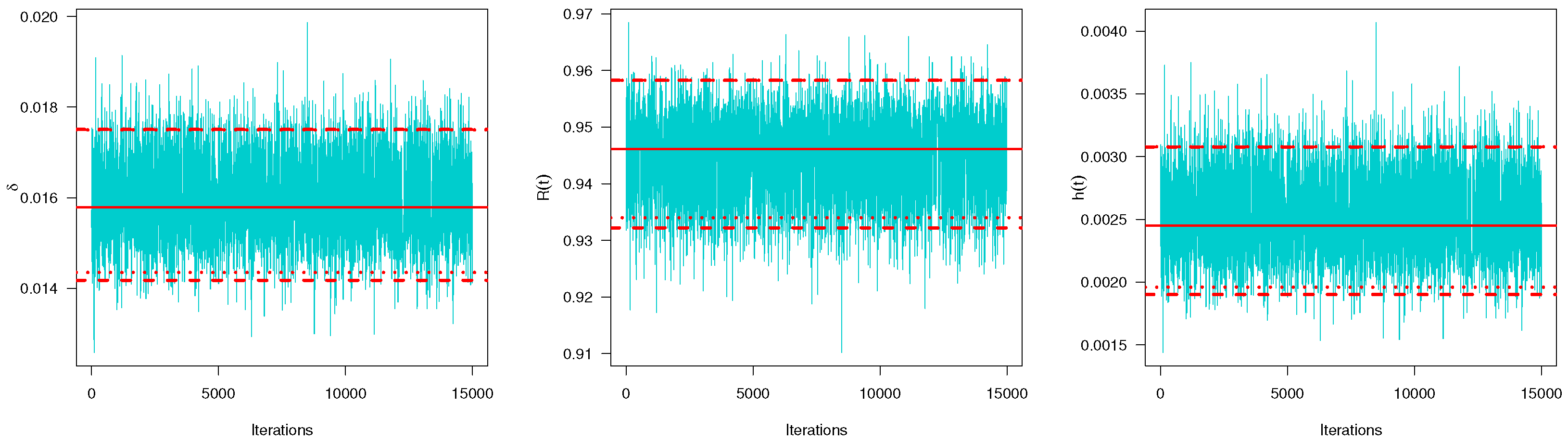
1 and 3, respectively. To develop the Bayesian computations, we generated 12,000 MCMC samples and then the first 2000 iterations were discarded from the generated sequence as burn-in to remove the affection of the selection of the initial value. Hence, the average BEs of the unknown parameters δ , R ( t ) and h ( t ) are computed based on the SEL function using 10,000 MCMC samples. The initial value of δ , for running the MCMC sampler algorithm, was taken to be its MLE. Moreover, for each n and m, different censoring schemes (CSs), R, to remove survival units during the lifetime experiment, are used as
CS - 1 : R 1 = n m , R i = 0 for i 1 , CS - 2 : R m 2 = n m , R i = 0 for i m / 2 , if m is even , R ( m + 1 ) 2 = n m , R i = 0 for i ( m + 1 ) / 2 , if m is odd , CS - 3 : R m = n m , R i = 0 f o r i m .
For each test, the average point estimates with their RMSEs and RABs as well as the ACWs of the interval estimates are given, respectively, by
η ^ r ¯ = 1 G i = 1 G η ^ r ( i ) , r = 1 , 2 , 3 ,
RMSE η ^ r = 1 G i = 1 G η ^ r ( i ) η r 2 , r = 1 , 2 , 3 ,
RAB η ^ r = 1 G i = 1 G 1 η r η ^ r ( i ) η r , r = 1 , 2 , 3 ,
and
ACW η ^ r = 1 G i = 1 G η ^ r U ( i ) η ^ r L ( i ) , r = 1 , 2 , 3 ,
where G is the number of replicates, η ^ is the MLE or BE of the parametric function η , η ^ r L , η ^ r U denote the 100 ( 1 ε ) % CI bounds, where η 1 = δ , η 2 = R ( t ) and η 3 = h ( t ) .
The average MLEs and BEs (Lindley’s and MCMC methods) of δ , R ( t ) and h ( t ) with their RMSEs and RABs are calculated and reported in Table 1, Table 2 and Table 3. In each table, the associated average estimate, RMSE and RAB, of any unknown parameter based on each test, are tabulated in the first, second, and third rows, respectively. Further, the ACWs of 95% asymptotic and credible intervals of δ , R ( t ) and h ( t ) are computed and listed in Table 4 and Table 5.
All numerical computations are performed using R statistical programming language software version 4.0.4 by mainly three useful recommended packages; namely (i) ‘CODA’ package, proposed by [37], used to carry out the Bayesian inference; (ii) ‘maxLik’ package, proposed by [38], used to obtain the MLEs via the N–R iterative procedure; and (iii) ‘GoFKernel’ package, proposed by [39], used to invert the xgamma distribution (2). These packages were recently recommended by [22,40,41,42,43].
From Table 1, Table 2 and Table 3, it can be seen that the proposed estimators of the unknown parameter and the reliability characteristics of XGD are very good, in terms of their RMSEs, RABs, and ACWs. As n (or m) increases, the RMSEs, RABs, and ACWs of both point and interval estimates decrease as expected. Thus, to get better estimation results, one may tend to increase the effective sample size. It is also observed that, as the failure percentage m / n increases, the point estimates become even better. Since the Bayes estimates of any parametric function include gamma prior information than the classical estimates, consequently, they perform better than the other competing estimates in terms of their RMSEs and RABs. Hence, the MCMC method using the M–H algorithm is better than Lindley’s approximation method, with respect to their RMSEs and RABs.
Regarding the xgamma parameter δ , RF R ( t ) , FRF h ( t ) , when δ increases with fixed T, the RMSEs and RABs associated with MLEs and BEs increase; moreover, they have similar behavior when T increases with fixed δ . When T increases with fixed δ , the RMSEs and RABs associated with MLE and Lindley estimates decrease, while those associated with the MCMC estimates increase. When T increases with fixed δ , the RMSEs and RABs associated with MCMC estimates increase, while those associated with MLEs and Lindley estimates decrease. From Table 4, Table 5 and Table 6, in respect to the interval estimates, the ACWs of asymptotic and credible intervals narrow down when n and m increases, as expected. In addition, as m / n increases, the 95% ACWs of all of the proposed estimates narrow down. As δ (or T) increases, the ACWs of both asymptotic and credible intervals for δ , R ( t ) , h ( t ) tend to increase. It can also be seen that the ACWs of asymptotic (NA/NL) intervals, as well as credible (BCI/HPD) intervals, are quite close to each other. Further, due to the gamma prior information, it is observed that the credible intervals perform better than the asymptotic intervals, with respect to the shortest ACWs, as expected.
Moreover, comparing schemes 1 and 3, it is clear that the RMSEs and RABs of all estimates for the unknown parameter δ , R ( t ) and h ( t ) are greater, based on scheme 3 than scheme 1. This is because the expected durations of the experiments using scheme 1, where the remaining n m units are withdrawn in the first stage, are greater than scheme 3, where the remaining n m units are withdrawn from the life test at the time of observed m-th failure. Finally, we recommend the Bayesian (point and interval) estimates of the unknown parameter and the reliability characteristics of the xgamma lifetime model using the M–H algorithm sampler.

6. Real-Life Applications

To show the adaptability and flexibility of the proposed methodologies to real phenomena, in this section, we provide two real datasets derived from the engineering and chemical fields.

6.1. Engineering Data Analysis

In this subsection, we discuss how the proposed methodology can be applied to a real-life phenomena by analyzing one real dataset given by [29]. This dataset shows that the cycle to failure numbers for 25 (100-cm) specimens of yarn tested at a particular strain level are: 15, 20, 38, 42, 61, 76, 86, 98, 121, 146, 149, 157, 175, 176, 180, 180, 198, 220, 224, 251, 264, 282, 321, 325, and 653. Before proceeding, we first fit the XGD to the complete yarn dataset along five popular lifetime models as competitors, namely: exponential E D ( δ ) , gamma G D ( α , δ ) , Weibull W D ( α , δ ) , generalized-exponential G E D ( α , δ ) and Nadarajah–Haghighi N H D ( α , δ ) , proposed by [44], distributions. Kolmogorov–Smirnov (K–S) distance with the associated p-value is used to check the validity of the proposed models. Further, several goodness-of-fit measures were also, namely: negative log-likelihood criterion (NLC) ( · ) , Akaike’s information criterion (AIC), A I C = 2 + 2 τ , consistent Akaike information criterion (CAIC), C A I C = 2 + ( 2 n τ / n τ 1 ) , Bayesian information criterion (BIC), B I C = 2 + τ log ( n ) , and Hannan–Quinn information criterion (HQIC), H Q I C = 2 + 2 τ log ( log ( n ) ) , where n and τ are the sample size and the dimension of the model parameter, respectively.
The maximum likelihood estimation method is used to estimate the unknown parameters of the considered distribution and to evaluate all terms of the model selection criteria. In general, the best distribution that provides the better fit corresponds to the lowest value of NLC, AIC, CAIC, BIC, HQIC, and K–S statistic values and highest p-values. The values of MLEs of the model parameters and corresponding goodness-of-fit measures are computed and reported in Table 7. It shows that the XGD fits the life cycle of the yarn dataset quite satisfactorily. Moreover, the XGD is the best choice among other competing models because it has the smallest K–S value with the highest p-value.
According to BIC, HQIC, and K–S (p-value), it can be seen that the XGD is the better choice, followed by gamma, generalized-exponential, exponential, Weibull, and Nadarajah–Haghighi distributions, respectively. Similarly, according to NLC, AIC, and CAIC, it is noted that the gamma distribution is slightly better than the other distributions. In addition, another advantage of using XGD, instead of the two-parameter competing distributions for modeling lifetime data, is that XGD only has one parameter. Consequently, from a computational point of view, inferential procedures become more convenient. For more illustration, we have provided two plots computed at the estimated model parameter(s) of each considered distribution. Plot (a) represents the empirical CDF plot and the fitted CDFs; Plot (b) represents the histogram of the yarn dataset and the fitted PDFs, see Figure 1. Now, we discuss the proposed estimates in the presence of the complete yarn dataset. Using different choices of m, T, and R, three APHCS-T2 samples are generated and presented in Table 8. In short, the censoring scheme R = ( 3 , 0 , 0 , 3 ) is referred as R = ( 3 , 0 * 2 , 3 ) . Because we lack prior information about the xgamma parameter, the approximate BEs are developed using Lindley and MCMC approximation methods under gamma improper, i.e., a = b = 0 .
Using the M–H algorithm described in Section 3.2, 20,000 MCMC samples were generated and the first 5000 iterations of the simulated variates were discarded as burn-in. Using Table 8, the MLEs and BEs with their standard errors (SEs) of the unknown parameters δ , R ( t ) and h ( t ) (at given mission time t = 50 ) are calculated and reported in Table 9. To run the MCMC sampler algorithm, the initial values of the unknown parameters were taken to be their MLEs. Moreover, two-sided 95% asymptotic and credible intervals with their lengths are computed, listed in Table 9. Recall that, in the literature, we have not come across a way to obtain the variance (or construct the associated interval) for the Lindley estimate. It shows that the point estimates of the unknown parameters obtained by MLEs and BEs are quite close to each other. Further, the interval estimates of δ , R ( t ) and h ( t ) obtained by 95% asymptotic/credible intervals are also similar.
Trace plot, or time-series diagram, is a simple way to judge how quickly the MCMC converges at each iteration with the iteration (x-axis) and the sampled values (y-axis). Hence, the trace plots of the simulated 15,000 samples of δ , R ( t ) and h ( t ) based on the complete yarn dataset are given in Figure 2. In each trace plot, the sample mean is displayed with a horizontal solid line (—), further, lower, and upper bounds of 95% BCIs and HPD credible intervals are displayed with dotted (⋯) and dashed (- - -) horizontal lines, respectively. It indicates that the MCMC procedure converges well; it also shows that discarding the first 5000 samples as burn-in is an appropriate size to erase the effect of the initial values. Moreover, it shows that the bounds of 95% BCI/HPD credible intervals are very close to each other. In addition, the histograms for the MCMC outputs of size 15,000 of δ , R ( t ) and h ( t ) , using the Gaussian kernel, are plotted in Figure 3. Similarly, in each histogram plot, the sample mean is displayed with a vertical solid line (|). It is evident from the estimates that the generated sequences of δ are fairly symmetric, while the generated sequences of R ( t ) and h ( t ) are close to negative and positively skewed, respectively. Furthermore, some properties of MCMC samples such as: mean, median, mode, SE, standard deviation (SD), and skewness (Sk.) of each unknown parameter are computed and displayed in Table 10. It indicates that the central tendency measures are quite close to each other. Thus, the proposed estimates support our findings and showed that the XGD has superior performance.

6.2. Chemical Data Analysis

This application provides an analysis of vinyl chloride, which is a known human carcinogen; exposure to this compound should be avoided as much as possible and its levels should be kept as low as technically feasible. However, according to [45], this dataset represents 34 data points (in mg/L) for vinyl chloride obtained from clean up-gradient monitoring wells, as: 0.1, 0.1, 0.2, 0.2, 0.4, 0.4, 0.4, 0.5, 0.5, 0.5, 0.6, 0.6, 0.8, 0.9, 0.9, 1.0, 1.1, 1.2, 1.2, 1.3, 1.8, 2.0, 2.0, 2.3, 2.4, 2.5, 2.7, 2.9, 3.2, 4.0, 5.1, 5.3, 6.8, 8.0. First, we need to check if the XGD is a suitable model to fit the vinyl chloride data or not. Thus, the K–S statistic, along with the associated p-value, is obtained. Using complete vinyl chloride data, the MLE (along its SE) of δ is 1.0313(0.1235); the K–S (along its p-value) is 0.138(0.533). This result indicates that the p-value is quite high compared to the significance level 5%, so we cannot reject the null hypothesis that the given data are coming from the XGD lifetime model. To get the proposed estimates, using m = 17 with different choices of T and R, three artificial APHCS-T2 samples are generated from the vinyl chloride dataset and are presented in Table 11. Using each generated sample, the MLEs and BEs with their SEs of δ , R ( t ) and h ( t ) (at distinct time t = 0.5 ) are calculated and reported in Table 12. Moreover, 95% two-sided asymptotic/credible interval estimates with their lengths are also computed and listed in Table 12. Here, we assume that prior information about the xgamma parameter δ is not available; the Bayes MCMC estimates with associated credible intervals are developed by run the chain of the MCMC sampler for 30,000 iterations, discarding the first 5000 values as a burn-in period. From, Table 12, it is seen that the Bayes MCMC estimates computed using Lindley and MCMC methods are very close to the corresponding MLEs. A similar pattern is observed with the interval (asymptotic/credible) estimates.
For graphical representation, using the complete vinyl chloride dataset, the trace and histogram plots of δ , R ( t ) and h ( t ) based on 25,000 MCMC simulated variates are plotted in Figure 4 and Figure 5, respectively. Figure 4 shows the convergence of MCMC outputs for each unknown parameter. It is also clear that, from Figure 5, the generated posteriors of all unknown parameters are fairly symmetric. Furthermore, some vital statistics of MCMC outputs are calculated and reported in Table 13. Finally, we conclude that the proposed methodologies, using both yarn and vinyl chloride datasets, provide a good demonstration of the unknown xgamma parameter and related reliability characteristics.

7. Concluding Remarks

In this paper, we have shown that the one-parameter xgamma distribution is a useful survival model for modeling reliability data. Moreover, we discussed the problem of estimating the unknown parameter and some reliability characteristics of the proposed xgamma model based on the adaptive type-II progressive hybrid censored samples. The maximum likelihood estimates with associated asymptotic confidence intervals of the unknown quantities were obtained numerically by the ‘maxLik’ package. The Lindley and Metropolis–Hastings approximation methods were used to approximate the Bayes estimates and to construct the associated credible intervals. In Bayesian computations, an algorithm used to determine the values of hyperparameters based on past samples was proposed.
To compare the behavior of the different estimates, a simulation study was conducted under various scenarios. The simulation results indicate that the Bayesian estimates perform better than the classical estimates in terms of minimum value of the root mean squared-error, relative absolute bias, and average confidence width. To demonstrate the applicability of the proposed methodologies in a real situation, two datasets related to engineering and chemical experiments were analyzed. Although we mainly considered adaptive type-II progressively hybrid censoring from the xgamma model, in future work, the same methods could be extended to other distributions and/or censoring plans. Finally, we hope that the results and methodology discussed in this paper will be beneficial to reliability practitioners.

Author Contributions

Methodology, A.E.; Funding acquisition, B.R.E.; Software, A.E.; Supervision, B.R.E.; Writing—original draft, A.E.; Writing—review & editing, A.E. and B.R.E. All authors have read and agreed to the published version of the manuscript.

Funding

This research received no external funding.

Data Availability Statement

The authors confirm that the data supporting the findings of this study are available within the article.

Acknowledgments

The authors would like to express thanks to the Editor-in-Chief, Special Issue Editor, and the anonymous referees for their careful reading and constructive comments, which led to this substantively improved version of the manuscript.

Conflicts of Interest

The authors declare no conflict of interest.

References

  1. Lindley, D.V. Fiducial distributions and Bayes’ theorem. J. R. Stat. Soc. Ser. B 1958, 20, 102–107. [Google Scholar] [CrossRef]
  2. McLachlan, G.; Peel, G. Finite Mixture Models; Wiley: New York, NY, USA, 2000. [Google Scholar]
  3. Sen, S.; Maiti, S.S.; Chandra, N. The xgamma distribution: Statistical properties and application. J. Mod. Appl. Stat. Methods 2016, 15, 774–788. [Google Scholar] [CrossRef] [Green Version]
  4. Sen, S.; Chandra, N.; Maiti, S.S. Survival estimation in xgamma distribution under progressively Type-II right censored scheme. Model Assist. Stat. Appl. 2018, 13, 107–121. [Google Scholar] [CrossRef]
  5. Yadav, A.S.; Saha, M.; Singh, S.K.; Singh, U. Bayesian estimation of the parameter and the reliability characteristics of xgamma distribution using Type-II hybrid censored data. Life Cycle Reliab. Saf. Eng. 2019, 8, 1–10. [Google Scholar] [CrossRef]
  6. Saha, M.; Yadav, A.S. Estimation of the reliability characteristics by using classical and Bayesian methods of estimation for xgamma distribution. Life Cycle Reliab. Saf. Eng. 2021, 10, 303–317. [Google Scholar] [CrossRef]
  7. Ng, H.K.T.D.; Chan, P.S. Statistical analysis of exponential lifetimes under an adaptive Type-II progressive censoring scheme. Nav. Res. Logist. 2009, 56, 687–698. [Google Scholar] [CrossRef] [Green Version]
  8. Hemmati, F.; Khorram, E. Statistical analysis of the log-normal distribution under Type-II progressive hybrid censoring schemes. Commun. Stat. Simul. Comput. 2013, 42, 52–75. [Google Scholar] [CrossRef]
  9. Mahmoud, M.A.W.; Soliman, A.A.; Abd-Ellah, A.H.; El-Sagheer, R.M. Estimation of generalized Pareto under an adaptive Type-II progressive censoring. Intell. Inf. Manag. 2013, 5, 73–83. [Google Scholar] [CrossRef] [Green Version]
  10. Ismail, A.A. Inference for a step-stress partially accelerated life test model with an adaptive Type-II progressively hybrid censored data from Weibull distribution. J. Comput. Appl. Math. 2014, 260, 533–542. [Google Scholar] [CrossRef]
  11. Ashour, S.K.; Nassar, M.M.A. Analysis of generalized exponential distribution under adaptive Type-II progressive hybrid censored competing risks data. Int. J. Adv. Stat. Probab. 2014, 2, 108–113. [Google Scholar] [CrossRef]
  12. Tian, Y.; Zhu, Q.; Tian, M. Estimation for mixed exponential distributions under Type-II progressively hybrid censored samples. Comput. Stat. Data Anal. 2015, 89, 85–96. [Google Scholar] [CrossRef]
  13. Sobhi, M.M.A.L.; Soliman, A.A. Infrared navigation-Part I: An assessment of feasibility. Appl. Math. Model. 2016, 40, 1180–1192. [Google Scholar]
  14. Zhang, C.; Shi, Y. Estimation of the extended Weibull parameters and acceleration factors in the step-stress accelerated life tests under an adaptive progressively hybrid censoring data. J. Stat. Comput. Simul. 2016, 86, 3303–3314. [Google Scholar] [CrossRef]
  15. Hemmati, F.; Khorram, E. On adaptive progressively Type-II censored competing risks data. Commun. Stat. Simul. Comput. 2017, 46, 4671–4693. [Google Scholar] [CrossRef]
  16. Nassar, M.; Abo-Kasem, O.E. Estimation of the inverse Weibull parameters under adaptive Type-II progressive hybrid censoring scheme. J. Comput. Appl. Math. 2017, 315, 228–239. [Google Scholar] [CrossRef]
  17. Nassar, M.; Abo-Kasem, O.E.; Zhang, C.; Dey, S. Analysis of Weibull distribution under adaptive Type-II progressive hybrid censoring scheme. J. Indian Soc. Probab. Stat. 2018, 19, 25–65. [Google Scholar] [CrossRef]
  18. Xu, R.; Gui, W. Entropy estimation of inverse Weibull distribution under adaptive Type-II progressive hybrid censoring schemes. Symmetry 2019, 11, 1463. [Google Scholar] [CrossRef] [Green Version]
  19. Kohansal, A.; Bakouch, H.S. Estimation procedures for Kumaraswamy distribution parameters under adaptive Type-II hybrid progressive censoring. Commun. Stat. Simul. Comput. 2019. [Google Scholar] [CrossRef]
  20. Panahi, H.; Moradi, N. Estimation of the inverted exponentiated Rayleigh distribution based on adaptive Type-II progressive hybrid censored sample. J. Comput. Appl. Math. 2020, 364, 112345. [Google Scholar] [CrossRef]
  21. Panahi, H.; Asadi, S. On adaptive progressive hybrid censored Burr Type-III distribution: Application to the nano droplet dispersion data. Qual. Technol. Quant. Manag. 2021, 18, 179–201. [Google Scholar] [CrossRef]
  22. Elshahhat, A.; Nassar, M. Bayesian survival analysis for adaptive Type-II progressive hybrid censored Hjorth data. Comput. Stat. 2021, 36, 1965–1990. [Google Scholar] [CrossRef]
  23. Kundu, D.; Pradhan, B. Bayesian inference and life testing plans for generalized exponential distribution. Sci. China Ser. A Math. 2009, 52, 1373–1388. [Google Scholar] [CrossRef] [Green Version]
  24. Lindley, D.V. Approximate Bayesian methods. Trab Estad. 1980, 31, 223–245. [Google Scholar] [CrossRef]
  25. Gelman, A.; Carlin, J.B.; Stern, H.S.; Rubin, D.B. Bayesian Data Analysis, 2nd ed.; Chapman and Hall/CRC: New Brunswick, NJ, USA, 2004. [Google Scholar]
  26. Lynch, S.M. Introduction to Applied Bayesian Statistics and Estimation for Social Scientists; Springer: New York, NY, USA, 2007. [Google Scholar]
  27. Kundu, D. Bayesian inference and life testing plan for the Weibull distribution in presence of progressive censoring. Technometrics 2008, 50, 144–154. [Google Scholar] [CrossRef]
  28. Dey, S.; Dey, T.; Luckett, D.J. Statistical inference for the generalized inverted exponential distribution based on upper record values. Math. Comput. Simul. 2016, 120, 64–78. [Google Scholar] [CrossRef]
  29. Lawless, J.F. Statistical Models and Methods for Lifetime Data, 2nd ed.; John Wiley and Sons: Hoboken, NJ, USA, 2003. [Google Scholar]
  30. Nelson, W. Applied Life Data Analysis; Wiley and Sons: New York, NY, USA, 1982. [Google Scholar]
  31. Meeker, W.Q.; Escobar, L.A. Statistical Methods for Reliability Data; John Wiley and Sons: New York, NY, USA, 1998. [Google Scholar]
  32. Krishnamoorthy, K.; Lin, Y. Confidence limits for stress-strength reliability involving Weibull models. J. Stat. Plan. Inference 2010, 140, 1754–1764. [Google Scholar] [CrossRef]
  33. Ahmed, E.A. Bayesian estimation based on progressive Type-II censoring from two-parameter bathtub-shaped lifetime model: A Markov chain Monte Carlo approach. J. Appl. Stat. 2014, 41, 752–768. [Google Scholar] [CrossRef]
  34. Lee, K.; Cho, Y. Bayesian and maximum likelihood estimations of the inverted exponentiated half logistic distribution under progressive Type II censoring. J. Appl. Stat. 2017, 44, 811–832. [Google Scholar] [CrossRef]
  35. Chen, M.H.; Shao, Q.M. Monte Carlo estimation of Bayesian credible and HPD intervals. J. Comput. Graph. Stat. 1999, 8, 69–92. [Google Scholar]
  36. Balakrishnan, N.; Sandhu, R.A. A simple simulation algorithm for generating progressive Type-II censored samples. Am. Stat. 1995, 49, 229–230. [Google Scholar]
  37. Plummer, M.; Best, N.; Cowles, K.; Vines, K. ‘Coda’: Convergence diagnosis and output analysis for MCMC. R News 2006, 6, 7–11. [Google Scholar]
  38. Henningsen, A.; Toomet, O. ‘maxLik’: A package for maximum likelihood estimation in R. Comput. Stat. 2011, 26, 443–458. [Google Scholar] [CrossRef]
  39. Pavia, J.M. Testing goodness-of-fit with the kernel density estimator: GoFKernel. J. Stat. Softw. 2015, 66, 1–27. [Google Scholar] [CrossRef]
  40. Elshahhat, A.; Ashour, S. Bayesian and non-Bayesian estimation for Weibull parameters based on generalized Type-II progressive hybrid censoring scheme. Pak. J. Stat. Oper. Res. 2016, 12, 213–226. [Google Scholar] [CrossRef] [Green Version]
  41. Abo-Kasem, O.E.; Elshahhat, A. Analysis of two Weibull populations under joint progressively hybrid censoring. Commun. Stat. Simul. Comput. 2021. [Google Scholar] [CrossRef]
  42. Elshahhat, A.; Rastogi, M.K. Estimation of parameters of life for an inverted Nadarajah–Haghighi distribution from Type-II progressively censored samples. J. Indian Soc. Probab. Stat. 2021, 22, 113–154. [Google Scholar] [CrossRef]
  43. Ashour, S.K.; El-Sheikh, A.A.; Elshahhat, A. Inferences and optimal censoring schemes for progressively first-failure censored Nadarajah-Haghighi distribution. Sankhyā A 2020. [Google Scholar] [CrossRef]
  44. Nadarajah, S.; Haghighi, F. An extension of the exponential distribution. Statistics 2011, 45, 543–558. [Google Scholar] [CrossRef]
  45. Bhaumik, D.K.; Kapur, K.; Gibbons, R.D. Testing parameters of a gamma distribution for small samples. Technometrics 2009, 51, 326–334. [Google Scholar] [CrossRef]
Figure 1. Plots of estimated PDFs and CDFs of XGD and its competing models under yarn dataset.
Symmetry 13 02112 g001
Figure 2. Trace plots of MCMC draws of δ , R ( t ) and h ( t ) under yarn dataset.
Symmetry 13 02112 g002
Figure 3. Histograms of δ , R ( t ) and h ( t ) from the yarn dataset.
Symmetry 13 02112 g003
Figure 4. Trace plots of MCMC draws of δ , R ( t ) and h ( t ) under chloride dataset.
Symmetry 13 02112 g004
Figure 5. Histograms of δ , R ( t ) and h ( t ) from vinyl chloride dataset.
Symmetry 13 02112 g005
Table 1. The average estimates of δ with their RMSEs and RABs.
nmCS δ = 1 δ = 3
T 1313
MLELindleyMCMCMLELindleyMCMCMLELindleyMCMCMLELindleyMCMC
301510.97530.98391.01470.99640.96771.01723.00333.01933.19813.11663.12513.2309
0.11400.06600.01650.14490.09760.01860.50090.46440.20210.56380.52650.2530
0.08970.03540.01470.10990.03850.01720.12620.11790.06600.14490.13700.0770
20.94450.97940.98400.99040.96791.01763.00963.02113.36473.09593.10203.3940
0.18750.12800.01660.14110.12190.01910.52900.48660.37240.56140.51910.4013
0.12680.07140.01600.11010.04750.01760.13620.12650.12160.14380.13460.1313
30.63550.63611.03091.03511.03311.05013.12953.11603.41383.09513.08663.4417
0.46440.46030.03130.17790.17380.05110.60800.53380.45100.57140.50330.4761
0.43640.43240.03090.13220.12970.05010.15430.13780.13790.14500.13010.1472
2410.97820.98801.00890.99430.98071.01333.00302.88393.09973.08063.09163.1984
0.09310.03140.00930.12260.04750.01600.48140.75670.11260.53690.50580.2032
0.07370.01920.00890.09550.02600.01490.12220.09780.03330.13550.12880.0661
20.82400.94771.01610.99500.98021.01613.00432.86873.26813.07623.08573.2944
0.25170.08620.01700.12560.05660.01830.49470.76250.30110.53090.49850.3137
0.21010.05740.01610.09800.02630.01610.12090.10970.08940.13510.12800.0982
30.70270.92171.02130.95030.92891.03313.06892.72463.36443.09743.09523.4000
0.31350.10920.02310.21190.16030.03710.56380.92280.40220.55010.49650.4545
0.29790.08310.02130.17800.08640.03310.14450.17630.12150.13900.12700.1333
804010.99140.99370.99860.99640.99461.00873.00262.98313.01353.06932.97332.9855
0.07540.03850.01050.09140.04520.01580.36870.11720.01590.40160.10990.0201
0.06020.03010.00890.07220.03650.01060.09750.02030.00460.10550.02330.0050
20.98680.99091.00721.00010.99521.01803.00082.98842.98563.04132.96262.9849
0.10700.06170.01450.09760.03760.02200.35390.10700.01790.40660.15700.0233
0.06660.02840.01180.07600.02880.01840.09270.02060.00490.10480.02630.0068
30.47050.47170.96841.01650.99280.97003.08102.94683.02133.05862.94763.0256
0.54410.54300.03270.10960.04610.03090.40270.22760.02600.41480.24360.0291
0.53360.53240.03160.08570.02610.03000.10460.04270.00730.10760.04310.0085
6410.99310.99551.00521.00040.99931.00282.98863.00442.99493.03373.01292.0121
0.05930.04110.00550.07670.05110.00680.27060.11000.00580.31910.12060.0180
0.04770.03290.00520.06060.04110.00600.07210.02990.00170.08450.03330.0044
20.74420.81210.99500.99250.99441.01682.99203.00432.99543.04553.01532.9887
0.30960.22990.00780.07570.04840.01700.28130.10120.00620.32210.10800.0219
0.27130.19830.00610.06010.03890.01680.07370.02760.00170.08230.02940.0065
30.65070.74461.02060.88170.91751.01653.00872.99662.99203.02643.00932.9759
0.35740.26470.02160.21230.13600.01770.34390.12460.00980.31040.07090.0286
0.34930.25540.02060.17980.10590.01650.08470.02360.00290.08210.01900.0082
Table 2. The average estimates of R ( t ) with their RMSEs and RABs.
nmCS δ = 1 δ = 3
T 1313
MLELindleyMCMCMLELindleyMCMCMLELindleyMCMCMLELindleyMCMC
301510.95390.95600.95130.95240.94800.95120.80500.80740.79050.79700.79890.7881
0.00780.03440.00110.01020.04440.00130.03550.03770.01450.03980.04160.0181
0.00650.02830.00110.00800.03180.00130.03370.03630.01770.03860.04060.0206
20.95580.96280.95340.95280.95000.95110.80460.80680.77860.79850.80040.7766
0.01210.05580.00120.00980.04790.00130.03750.04000.02660.03970.04180.0287
0.00890.04280.00120.00800.03480.00130.03650.03930.03240.03830.04060.0350
30.97480.97480.95020.94970.94910.94890.79620.79720.77520.79860.79970.7733
0.02930.02990.00220.01250.01320.00360.04270.04630.03210.04030.04370.0339
0.02910.02970.00230.00970.01010.00370.04100.04470.03660.03860.04220.0391
2410.95380.95570.95170.95260.95080.95140.80500.81080.79750.79950.80140.7904
0.00640.02020.00060.00850.03060.00110.03410.09310.00810.03790.03950.0146
0.00530.01670.00060.00690.02290.00100.03270.09130.00900.03610.03800.0177
20.96380.98700.95120.95260.95060.95120.80490.81100.80600.79980.80160.7836
0.01650.05010.00120.00870.03330.00130.03500.09870.02150.03750.03930.0224
0.01460.04550.00110.00710.02500.00120.03240.09310.02390.03610.03790.0262
30.97180.99950.95090.95530.95350.95000.80040.79640.77870.79830.79970.7762
0.02040.06150.00160.01430.06530.00250.04020.12400.02870.03880.04160.0323
0.02040.06340.00150.01270.05520.00240.03870.12290.03230.03710.04000.0354
804010.95290.95340.95240.95250.95230.95170.80480.80830.80370.80010.79800.8058
0.00520.01210.00070.00630.01500.00110.02640.05380.00110.02870.05710.0015
0.00440.01010.00060.00520.01200.00080.02620.05410.00120.02830.05640.0014
20.95310.95390.95180.95230.95160.95110.80490.80900.80580.80210.80230.8058
0.00690.01610.00100.00680.01920.00150.02540.05460.00130.02900.06120.0017
0.00470.01210.00090.00550.01460.00130.02490.05420.00130.02810.05960.0018
30.98490.98510.95450.95110.94740.95440.79920.79640.80320.80080.80040.8029
0.03340.03350.00230.00770.03320.00210.02870.06850.00190.02960.07060.0021
0.03450.03470.00230.00630.02630.00220.02800.06770.00200.02880.06980.0023
6410.95280.95320.95200.95230.95210.95210.80570.80870.80510.80250.80320.8038
0.00410.00740.00040.00530.01000.00050.01950.03280.00040.02290.03810.0013
0.00350.00630.00040.00440.00810.00040.01940.03280.00050.02270.03780.0012
20.96890.98150.95270.95280.95320.95120.80540.80850.80500.80160.80180.8055
0.02010.03500.00050.00520.01020.00120.02020.03470.00050.02300.03900.0016
0.01860.03280.00040.00440.00840.00120.01990.03430.00050.02210.03750.0017
30.97500.99250.95090.96010.96690.95120.80430.80660.80530.80300.80460.8065
0.02310.04050.00150.01410.02890.00120.02490.04520.00070.02230.04160.0021
0.02380.04210.00140.01260.02680.00120.02280.04230.00080.02210.04150.0022
Table 3. The average estimates of h ( t ) with their RMSEs and RABs.
nmCS δ = 1 δ = 3
T 1313
MLELindleyMCMCMLELindleyMCMCMLELindleyMCMCMLELindleyMCMC
301510.46150.46020.48780.47710.44960.48962.10822.09492.27432.60702.18362.3029
0.07920.05490.01170.10420.08560.01320.43570.38710.17540.49140.43440.2199
0.13110.05850.02180.16300.06760.02540.15590.14220.08180.17950.16240.0954
20.44310.45140.46620.47280.44930.48992.11412.09462.41962.18912.16182.4452
0.12250.10510.01170.10020.10470.01350.46000.40430.32390.48890.42740.3492
0.17970.11470.02350.16250.08200.02620.16840.15210.15090.17790.15930.1631
30.25170.24940.49930.50540.50280.51302.21862.16382.46282.18852.13972.4872
0.29560.29480.02220.12810.12320.03630.53050.43230.39300.49780.40880.4150
0.58540.58450.04590.19730.19110.07450.19120.16100.17140.17950.15230.1830
2410.46310.46820.48370.47500.46140.48682.10781.94002.18892.17552.15912.2746
0.06500.02280.00660.08740.04010.01130.41870.88720.09770.46790.42130.1764
0.10800.02850.01310.14130.04190.02210.15090.15600.04120.16780.15440.0819
20.36170.43750.48880.47560.46060.48882.10901.92162.33542.17172.15282.3584
0.16640.06370.01200.08940.04900.01300.43040.87280.26190.46220.41450.2728
0.29380.09040.02390.14490.04370.02380.14940.17290.11080.16720.15300.1217
30.28090.41840.49250.44770.41750.50102.16611.75892.41952.19022.15352.4509
0.20610.08020.01630.14580.13500.02630.48851.03730.35030.47930.40740.3963
0.41260.13030.03150.25780.14770.04930.17850.27400.15080.17220.15030.1657
804010.47200.47290.47650.47580.47330.48362.10642.06502.11412.16432.04792.0899
0.05300.02620.00740.06480.03060.01120.31970.14610.01370.34890.14240.0174
0.08870.04280.01310.10670.05170.01570.12050.02950.00570.13060.03580.0062
20.46970.47090.48250.47850.47320.49022.10472.06892.08992.14022.03742.0894
0.07020.04120.01020.06950.02670.01560.30680.13990.01550.35320.20450.0202
0.09620.03960.01750.11250.04070.02730.11450.03300.00610.12960.04350.0084
30.15000.15090.45530.49040.46900.45642.17452.01142.12082.15522.01382.1246
0.33530.33430.02290.07840.04060.02170.35010.28580.02250.36040.30380.0252
0.69220.69010.04640.12740.04590.04410.12950.07540.00910.13300.07550.0105
6410.47300.47440.48110.47830.47700.47942.09352.09692.09802.13292.09972.1129
0.04160.02840.00390.05440.03530.00480.23420.08120.00500.27680.08700.0156
0.07030.04770.00760.08970.05970.00890.08890.03050.00210.10440.03300.0055
20.31000.35120.47390.47280.47350.48932.09652.09582.09842.14312.10002.0926
0.20240.15400.00550.05350.03340.01200.24370.07270.00540.27970.07930.0190
0.37390.27940.00910.08870.05630.02490.09100.02730.00210.10170.02860.0080
30.24840.30580.49200.39970.42080.48912.11162.08292.09552.12652.09362.0816
0.23350.17730.01530.14240.09220.01250.29640.10340.00850.26900.05160.0247
0.47970.35950.03050.25550.15030.02450.10440.02300.00350.10150.01730.0101
Table 4. The ACWs for 95% asymptotic/credible interval estimates of δ .
δ nmCS T = 1 T = 3
AsymptoticCredibleAsymptoticCredible
NANLBCIHPDNANLBCIHPD
1301510.67660.69020.02170.02160.61950.62950.02580.0257
20.65090.66390.01600.01590.61420.62410.02630.0262
30.38520.39130.01750.01730.63510.64510.04470.0412
2410.53700.54380.01100.01020.54870.55570.03250.0320
20.43730.44250.02130.02080.54870.55570.02980.0292
30.35910.36300.03010.03000.50920.51540.04960.0495
804010.42230.42550.03350.03340.42550.42870.04100.0409
20.41950.42270.04040.04030.42700.43020.03790.0378
30.16390.16470.02940.02880.43040.43360.02900.0287
6410.33470.33630.00710.00690.33790.33950.01830.0182
20.23870.23980.01960.01950.33460.33620.01050.0104
30.20260.20340.02460.02340.28570.28690.02130.0209
3301512.05702.09750.17620.16222.14472.18730.39190.3898
22.06812.10910.34630.32522.13512.17780.37040.3189
32.17792.22220.53720.53492.15102.19460.58480.5841
2711.92361.95670.18160.18111.97972.01400.15840.1563
21.92841.96180.44850.43881.98042.01490.37120.3696
31.98062.01520.49330.49292.00522.04050.64950.6493
804011.48831.50360.02770.02761.52591.54170.04680.0465
21.49201.50740.03360.03271.51481.53060.05770.0574
31.55361.57010.04640.04511.54091.55730.04580.0457
6411.16991.17730.01110.01101.19001.19760.05070.0497
21.17391.18140.01490.01481.19781.20560.07740.0725
31.18511.19280.02230.02221.19441.20220.05280.0576
Table 5. The ACWs for 95% asymptotic/credible interval estimates of R ( t ) .
δ nmCS T = 1 T = 3
AsymptoticCredibleAsymptoticCredible
NANLBCIHPDNANLBCIHPD
1301510.00010.12230.00150.00150.00010.11100.00180.0017
20.00010.11730.00110.00100.00010.11020.00180.0018
30.00010.06770.00120.00120.00020.11230.00310.0029
2410.00010.09720.00080.00070.00010.09860.00230.0022
20.00010.07800.00150.00140.00010.09860.00210.0020
30.00010.06690.00210.00200.00010.09100.00350.0034
804010.00010.07630.00230.00220.00010.07670.00290.0028
20.00010.07570.00280.00270.00010.07680.00260.0026
30.00010.02870.00200.00190.00010.07710.00200.0019
6410.00010.06050.00050.00040.00010.06090.00130.0012
20.00010.04390.00140.00130.00010.06040.00070.0007
30.00010.03770.00170.00160.00010.05190.00150.0014
3301510.00020.16670.01260.01160.00020.16490.02790.0278
20.00020.16680.02460.02310.00020.16560.02620.0225
30.00020.16600.03800.03780.00020.16680.04120.0411
2410.00010.15610.01310.01300.00020.15480.01130.0112
20.00020.15630.03190.03130.00020.15520.02630.0262
30.00020.15480.03490.03480.00020.15550.04570.0457
804010.00010.12150.00200.00190.00010.12080.00340.0034
20.00010.12200.00240.00230.00010.12140.00420.0041
30.00010.12240.00340.00320.00010.12250.00330.0033
6410.00010.09650.00080.00080.00010.09610.00370.0036
20.00010.09670.00110.00100.00010.09620.00560.0052
30.00010.09640.00160.00160.00010.09670.00420.0041
Table 6. The ACWs for 95% asymptotic/credible interval estimates of h ( t ) .
δ nmCS T = 1 T = 3
AsymptoticCredibleAsymptoticCredible
NANLBCIHPDNANLBCIHPD
1301510.48850.51170.01540.01530.45150.46840.01830.0182
20.46760.48960.01120.01110.44640.46310.01870.0186
30.24510.25500.01250.01230.46930.48640.03190.0295
2410.38790.39930.00770.00720.39900.41080.02300.0226
20.22920.30780.01510.01480.39910.41100.02120.0207
30.22870.23510.02130.02130.36670.37710.03530.0352
804010.30630.31170.02360.02350.30920.31480.02910.0290
20.30430.30970.02860.02850.31080.31630.02690.0268
30.08730.08730.02060.02010.31520.32060.02030.0201
6410.24280.24550.00500.00480.24590.24860.01290.0129
20.15700.15870.01380.01370.24280.24550.00750.0074
30.12460.12590.01740.01660.20000.20210.01510.0148
3301511.97972.05330.15310.14102.08062.15860.34130.3394
21.99202.06660.30210.28382.06872.14660.32350.2789
32.11612.19740.46930.46722.08442.16420.51160.5110
2411.85061.91070.15750.15711.91551.97810.13770.1360
21.85581.91640.39090.38221.91551.97830.32400.3225
31.91631.97950.43070.43041.94272.00710.56810.5679
804011.42971.45730.02390.02391.47261.50120.04050.0402
21.43281.46060.02910.02831.45951.48790.04990.0497
31.50041.53040.04020.03891.48641.51600.03970.0396
6411.12161.13510.00960.00951.14481.15860.04380.0431
21.12581.13940.01280.01281.15331.16720.06700.0627
31.13861.15250.01930.01921.14841.16250.05040.0498
Table 7. Summary fit for the life cycle of the yarn dataset.
ModelMLENLCAICCAICBICHQICK–S
α ^ δ ^ Statisticp-Value
XGD-0.0166154.16310.32310.49309.72308.610.11880.8722
GD1.79900.0101152.44308.88309.42311.31309.550.13880.7209
GED1.88630.0081152.49308.98309.53311.42309.660.14370.6806
WD1.12830.0028153.41310.83311.37313.27311.500.17900.3997
NHD1.64940.0029153.56311.11311.66313.55311.790.18340.3697
ED-0.0056154.59311.18311.35312.40311.520.19900.2753
Table 8. Three different APHCS-T2 samples generated from the yarn dataset.
Samplem T ( d ) R R m * Censored Data
1880(6) R = ( 17 , 0 * 7 ) 015, 224, 251, 264, 282, 321, 325, 653
211140(9) R = ( 7 , 0 * 9 , 7 ) 715, 121, 146, 149, 157, 175, 176, 180, 180, 198, 220
315200(17) R = ( 0 * 14 , 10 ) 1015, 20, 38, 42, 61, 76, 86, 98, 121, 146, 149, 157, 175, 176, 180
Table 9. The point estimates (SEs) and 95% interval estimates (lengths) under the yarn dataset.
SampleParameterMLELindleyMCMCAsymptoticCredible
NABCI
NLHPD
1 δ 0.0100(2.07 × 10 3 )0.01010.0099(6.29 × 10 7 )(0.0059,0.0141)[0.0081](0.0098,0.0102)[0.0004]
(0.0067,0.0150)[0.0083](0.0098,0.0102)[0.0004]
R ( 50 ) 0.9818(8.39 × 10 3 )0.98180.9819(2.78 × 10 6 )(0.9654,0.9983)[0.0329](0.9810,0.9827)[0.0017]
(0.9655,0.9984)[0.0329](0.9810,0.9827)[0.0017]
h ( 50 ) 0.0008(2.66 × 10 4 )0.00090.0008(1.27 × 10 7 )(0.0003,0.0013)[0.0010](0.0008,0.0009)[0.0001]
(0.0004,0.0016)[0.0012](0.0008,0.0009)[0.0001]
2 δ 0.0104(1.59 × 10 3 )0.01040.0103(6.32 × 10 7 )(0.0073,0.0136[0.0063])(0.0102,0.0106)[0.0004]
(0.0077,0.0141)[0.0064](0.0102,0.0106)[0.0004]
R ( 50 ) 0.9799(6.86 × 10 3 )0.97990.9800(2.95 × 10 6 )(0.9664,0.9934)[0.0270](0.9791,0.9810)[0.0019]
(0.9665,0.9935)[0.0270](0.9792,0.9810)[0.0018]
h ( 50 ) 0.0009(2.16 × 10 4 )0.00120.0009(1.35 × 10 7 )(0.0005,0.0013)[0.0008](0.0008,0.0010)[0.0002]
(0.0006,0.0015)[0.0009](0.0008,0.0009)[0.0001]
3 δ 0.0136(1.77 × 10 3 )0.01360.0135(9.10 × 10 6 )(0.0101,0.0170)[0.0069](0.0108,0.0164)[0.0056]
(0.0105,0.0175)[0.0070](0.0107,0.0163)[0.0056]
R ( 50 ) 0.9623(1.08 × 10 2 )0.96230.9621(5.99 × 10 5 )(0.9412,0.9834)[0.0422](0.9414,0.9781)[0.0367]
(0.9414,0.9836)[0.0422](0.9432,0.9793)[0.0361]
h ( 50 ) 0.0017(3.18 × 10 4 )0.00240.0017(2.72 × 10 6 )(0.0011,0.0023)[0.0012](0.0010,0.0026)[0.0016]
(0.0012,0.0025)[0.0013](0.0009,0.0025)[0.0016]
Table 10. Some posterior characteristics of MCMC outputs under the yarn dataset.
ParameterMeanMedianModeSESDSk.
δ 0.015790.015770.01432 7.02 × 10 6 8.60 × 10 4 0.08059
R ( 50 ) 0.946120.946530.95718 5.49 × 10 5 6.73 × 10 3 −0.26343
h ( 50 ) 0.002450.002430.00195 2.48 × 10 6 3.04 × 10 4 0.25825
Table 11. Three different APHCS-T2 samples generated from the vinyl chloride dataset.
Sample T ( d ) R R m * Censored Data
10.7(12) R = ( 1 * 17 ) 50.1, 0.2, 0.4, 0.4, 0.5, 0.6, 0.8, 0.9, 1.1, 1.2,
1.8, 2.0, 2.4, 2.5, 2.7, 2.9, 3.2
21.0(15) R = ( 9 , 0 * 15 , 8 ) 80.1, 0.6, 0.6, 0.8, 0.9, 0.9, 1.0, 1.1, 1.2, 1.2,
1.3, 1.8, 2.0, 2.0, 2.3, 2.4, 2.5
31.5(20) R = ( 0 * 8 , 17 , 0 * 8 ) 00.1, 0.1, 0.2, 0.2, 0.4, 0.4, 0.4, 0.5, 0.5, 2.7,
2.9, 3.2, 4.0, 5.1, 5.3, 6.8, 8.0
Table 12. The point estimates (SEs) and 95% interval estimates (lengths) under a vinyl chloride dataset.
SampleParameterMLELindleyMCMCAsymptoticCredible
NABCI
NLHPD
1 δ 0.8099(1.29 × 10 1 )0.80710.8167(2.32 × 10 4 )(0.5573,1.0626)[0.5052](0.7423,0.8762)[0.1340]
(0.5929,1.1064)[0.5135](0.7392,0.8724)[0.1332]
R ( 0.5 ) 0.8464(7.23 × 10 5 )0.84620.8447(6.10 × 10 5 )(0.8463,0.8466)[0.0003](0.8289,0.8642)[0.0353]
(0.8463,0.8466)[0.0003](0.8299,0.8650)[0.0351]
h ( 0.5 ) 0.3145(7.93 × 10 2 )0.31290.3186(1.34 × 10 4 )(0.1592,0.4699)[0.3107](0.2759,0.3534)[0.0775]
(0.1919,0.5154)[0.3235](0.2741,0.3511)[0.0770]
2 δ 0.8990(1.45 × 10 1 )0.89680.8909(1.18 × 10 5 )(0.6143,1.1837)[0.5694](0.8874,0.8943)[0.0067]
(0.6550,1.2340)[0.5790](0.8876,0.8944)[0.0068]
R ( 0.5 ) 0.8229(1.30 × 10 3 )0.82280.8250(3.14 × 10 6 )(0.8203,0.8254)[0.0051](0.8241,0.8260)[0.0019]
(0.8203,0.8254)[0.0051](0.8241,0.8259)[0.0018]
h ( 0.5 ) 0.3671(9.30 × 10 2 )0.36550.3622(7.07 × 10 6 )(0.1847,0.5494)[0.3647](0.3601,0.3642)[0.0041]
(0.2233,0.6032)[0.3799](0.3602,0.3643)[0.0041]
3 δ 0.7403(1.19 × 10 1 )0.73660.7400(1.60 × 10 5 )(0.5059,0.9748)[0.4689](0.7342,0.7442)[0.0099]
(0.5394,1.0162)[0.4768](0.7347,0.7445)[0.0098]
R ( 0.5 ) 0.8647(9.96 × 10 4 )0.86450.8648(4.18 × 10 6 )(0.8627,0.8667)[0.0039](0.8637,0.8663)[0.0026]
(0.8627,0.8667)[0.0039](0.8636,0.8662)[0.0026]
h ( 0.5 ) 0.2748(7.09 × 10 2 )0.27280.2746(9.00 × 10 6 )(0.1358,0.4137)[0.2779](0.2714,0.2770)[0.0056]
(0.1657,0.4557)[0.2900](0.2716,0.2771)[0.0055]
Table 13. Some vital statistics of MCMC outputs under the vinyl chloride dataset.
ParameterMeanMedianModeSESDSk.
δ 1.030291.030281.02851 6.31 × 10 6 9.97 × 10 4 0.03429
R ( 0.5 ) 0.788030.788040.78851 1.67 × 10 6 2.64 × 10 4 −0.03414
h ( 0.5 ) 0.447410.447400.44629 3.94 × 10 6 6.23 × 10 4 0.03508
Publisher’s Note: MDPI stays neutral with regard to jurisdictional claims in published maps and institutional affiliations.

