
The Surjective Mapping Conjecture and the Measurement Problem in Quantum Mechanics


Department Physik, University Siegen, 57076 Siegen, Germany
Symmetry 2021, 13(11), 2155; https://0-doi-org.brum.beds.ac.uk/10.3390/sym13112155
Submission received: 10 September 2021
/
Revised: 12 October 2021
/
Accepted: 1 November 2021
/
Published: 11 November 2021
(This article belongs to the Special Issue Quantum Mechanics: Concepts, Symmetries, and Recent Developments)
Abstract
:Accepting a time-symmetric quantum dynamical world with ontological wave functions or fields, we follow arguments that naturally lead to a two-boundary interpretation of quantum mechanics. The usual two boundary picture is a valid superdeterministic interpretation. It has, however, one unsatisfactory feature. The random selection of a chosen measurement path of the universe is far too complicated. To avoid it, we propose an alternate two-boundary concept called surjective mapping conjecture. It takes as fundamental a quantum-time running forward like the usual time on the wave-function side and backward on the complex conjugate side. Unrelated fixed arbitrary boundary conditions at the initial and the final quantum times then determine the measurement path of the expanding and contracting quantum-time universe in the required way.
1. Introduction
The wave function and the fields are the draft horses of quantum mechanics and quantum field theory. We here take a realist view about their ontological existence. Measurement decisions involving collapses require the elimination of wave function components all the way back. So, the realist view requires backward causation. The wave function and its conjugate follow the Schrödinger equation, which is entirely symmetric in time. For field theory, with its Hamilton function, the situation is analogous.
To accept time symmetry is a severe step. It involves some non-locality. Interpretations used different strategies to get around it. The Copenhagen interpretation tries to avoid backward causation by denying wave function ontological existence. In “An intricate quantum statistical effect and the foundation of quantum mechanics” [1], we argued that it is not successful in a broader quantum statistical domain and that backward causation is unavoidable. The basic argument is: If identical particles are produced with a certain probability at the time one can decide at a later time to allow them to mingle or to keep them separate. This decision at the time introduces or prevents interference terms which enhance or deplete the production probability a the time . As particle production is ontological, it means backward causation. In some way, the acceptance of time symmetry on a quantum level is a paradigm change. As we argued in “Time Symmetric Quantum Mechanics and Causal Classical Physics” [2], there is nothing wrong with time-symmetric quantum mechanics as long in our rapidly expanding universe an approximate classical time directed physics can be obtained.
The term “conjecture” instead of “interpretation” was used as there might be unthought-of problems. The most dangerous aspects are infinities which often lead to problems if involved limits are not considered carefully. We, therefore, decided to take the universe as finite with a vast lifetime from a big bang to a highly extended final state. As the universe is almost empty and sparsely interacting at its end, the limit presumably exists but is not taken.
As Sakurai [3] pointed out, most of the spectacular successes of Quantum Mechanics (QM) lie in the domain of Quantum Dynamics (QD), meaning QM without the Measurement Process involving collapses. Many applications of QM involve just static situations, and for most processes, one just needs to know the given initial and the possible final states.
2. The Components of Measurements
Nobody doubts QD; differences in interpretations concern the Theory of Measurements. There is a lot of splitting and merging in QD in which no components are eliminated. Such eliminations are an essential element of Measurement Processes. Empirically one knows that such measurement processes in which components disappear require witnesses. Usually, witnesses are observers who remember the choices taken. Here they can be just objects whose existence documents past selections.
Some basic facts about witnesses seem not fully realized. The fastest witness production involves phase changes [4]. For traceable witnesses, the by far dominant part is low-energy photons. Any drift chamber, any circuit board, and, if he visits, Wigner’s friend’s brain all emit measurable radiofrequency electromagnetic waves.
Individual photons with a radio wavelength between and 20 m carry unmeasurable energies of and Joule. There have to be a lot of them, and there are known to be penetrating. A substantial fraction of them will escape the apparatus, the laboratory, and there is a special window for these frequencies in the ionosphere. In our expanding universe, it means a large number of them will enter a part of the sky where they will never encounter any interaction. In this way, the information of the measurement will be stored in the final state. The final hypersphere () is enormous and even a single photon will somehow reversed point to the precise emission region reflecting the measurement decision. The stored information will not be disturbed by other particles. The same applies to the other measurements. As emission takes a specific time, the number of measurements in a finite universe is a finite huge number, say, for “zillion”. In an expanding universe grows faster than its lifetime.
A measurement result will be definite, such as up or down. It means the same choice on the wavefunction side and the complex conjugated one as described by the following projection:
To just add such an operator is not acceptable. It eliminates contributions that can only be done in processes involving witnesses.
However, in a finite universe, no problem arises. The final state on the wave-function side has to agree with that on the complex conjugated one. So, no mixed terms can contribute, e.g., with ↑ witnesses on the wave-function side and with ↓ witnesses on the other side. Formally for an unconstrained universe, one can replace the sum over all final states by a unit operator connecting the wavefunction and the complex conjugate one as done in Equation (2), depicting the evolution of the wave function and its complex conjugate part.
or
That the witnesses on both sides have to agree to contribute is now apparent. I kept the unit matrix to remember the separation. The argument stayed entirely in the domain of QD, and no addition was needed.
Next, the measurement will have to determine an actual choice, like a projection operator which takes ↑ and eliminates ↓:
At what time should the operator act? Clearly, this should occur outside of the quantum domain where all components are needed. This means it should occur behind a good part of the witness production, but it can be later. As there is backward causation, the only requirement is that states coming from the chosen component can be distinguished from the unchosen one. As some witnesses stay forever, it is possible to move the projection to the end, i.e., just before .
With everything except these measurement decisions integrated out, the number of measurement-decision paths in the universe will again be a finite number like . Of course, it is somewhat lower as there are correlations in measurement results like that of Alice and Bob and non-binary choices?
3. Two Boundary Quantum Dynamics
If we put all measurement projections to the end, we have QD everywhere except at the boundaries. One can define a final density operator containing all those projections and formally obtain the two-boundary interpretation [5,6,7,8] of QM. It is a serious, valid, super-deterministic interpretation of QM [9].
An unpleasant feature with these and similar theories is the required random selection of measurement path determined by the final boundary. For each measurement path i, it has to obtain the absolute square . Witnesses prevent interference contributions. It has then to choose a random number and determine the chosen J so that . In our opinion, it is far too complicated to be attractive.
There is a modified two-boundary interpretation, the surjective mapping conjecture, which avoids this unpleasant random choice. No measurement choice projections are needed. It takes the quantum time as fundamental and replaces the usual expression for the density.
by
For simplicity we inserted the definitions of the arguments. The mapping involved is in the set theory called surjection. With the condition:
the usual description would be obtained.
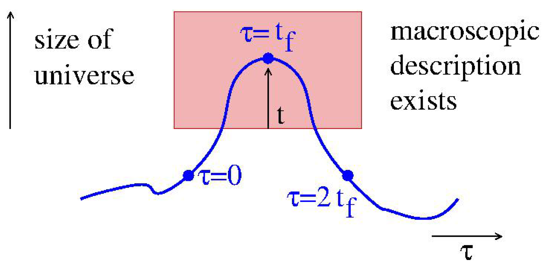
Equation (4) trivially holds around the unit operator for .The highly extended state at with all its witnesses strongly influences the smaller universe around it to keep Equation (4) sufficiently accurate for a large part of the universe, including our epoch. Where approximately valid, Equation (4) allows for a macroscopic description.
The formalism removes the constrain of this Equation (4). It allows for unequal boundaries at the initial and final quantum time:
They are result from a missing theory of the total quantum universe depicted in Figure 1.
One can evolve and revolve both boundary states to the state of maximum extend :
In the conventional quantum theory, they would be equal, and their product would be one. Now both sides are unrelated. Each occupies a tiny fraction of the vast phase space of the universe at , presumably of the order of . No overlap is expected except for an extremely tiny region:
There is no reason for the product to vanish.
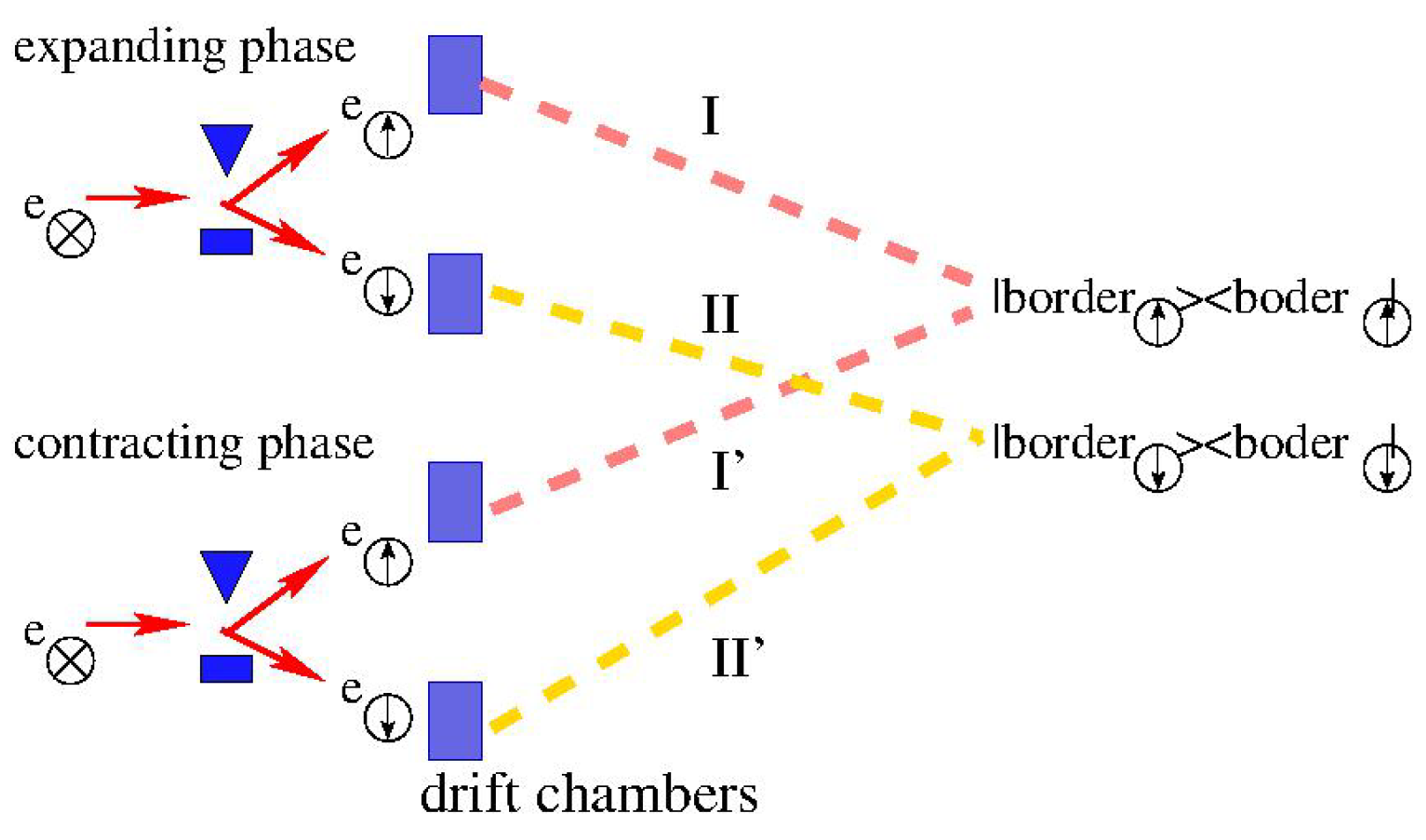
It changes the picture of measurements. Consider a generic Stern-Gerlach experiment shown in Figure 2 separately showing the wave function and the complex conjugate side. They are split in an inhomogeneous magnetic field and then enter drift chambers, where witnesses connected to the border state at fix a choice observable by charge coupled electronics. The setup of the initial particle to a spin ⊗ is common to both outcomes, ↑ and ↓, and can be ignored on both sides. The spin ↑-component and its future on both sides, the wave function and the conjugate one, following the dotted red line is then given in Equation (5):
An analogue expression holds for the spin ↓-component. The limited overlap at makes both terms tiny.
For statistical reasons, two independent, very tiny quantities are extremely unlikely of the same magnitude. So one will be dominant and the other irrelevant. (Exceptional situations—we ignore—might lead to multi-world choice between coexisting observers.) It looks like a random process choosing one and collapsing the other, but it reflects the influence of the available future paths.
This situation is not unimportant. A discontinuous dynamical evolution of the universe, i.e., one with jumps, is considered unacceptable on philosophical grounds. Furthermore, Einstein and other important physicists could not accept QM as a complete theory as it involved random dynamics, i.e., as “der Alte würfelt nicht”. The Surjective Mapping Conjecture avoids random dynamics and offers the envisioned completion.
The boundaries at the initial and final quantum-times are fixed. We can still average over many settings with different positions in the universe. The first and last factor in Equation (5) is known to be independent of settings and can be pulled out. As the process is basically symmetric one has for the average of the remaining factors:
It means the relative probability is given just by the first and last factors:
as required by the Born rule. It comes out automatically, no special choice had to be made.
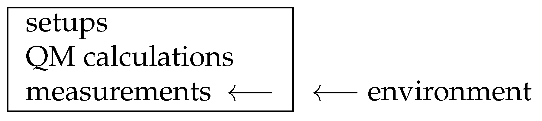
It reflects a general statistical property of QM (in Figure 3). For any setup with a measurement defined by witnesses reaching these witnesses, in turn, allow the matching at to determine individual measurements unpredictably:
No predictions are possible. Averaging, however, eliminates this seemingly random influence of the environment, and predictive calculations are possible.
It is in some way a hidden variable theory. However, the hidden variable
does not sit on individual particles where they would create problems [10]. It produces a narrow overlap region at . which determines all measurements, like in the usual two-boundary picture.
It is intrinsically somewhat less deterministic than the usual two boundary interpretations [11]. What happens at a time and affects the evolution in between, including the “final” state. So, if one likes, one can add or imagine to have added something like an outside, free-willed manipulation affecting this “final” state.
4. Conclusions
To conclude, as a multi-particle physicist analysing Bose–Einstein correlations, I was forced to accept backward causation. Backward causation and, consequently, non-locality changes paradigms in the interpretation of QM, suggesting a two-boundary interpretation. This note showed how a particular choice of boundaries could eliminate an un-pleasant feature of this interpretation.
Funding
This research received no external funding.
Institutional Review Board Statement
Not applicable.
Informed Consent Statement
Not applicable.
Data Availability Statement
Not applicable.
Acknowledgments
I have to thank many colleagues for fruitful discussions.
Conflicts of Interest
The authors declare no conflict of interest.
References
- Bopp, F.W. An intricate quantum statistical effect and the foundation of quantum mechanics. arXiv 2019, arXiv:1909.01391. [Google Scholar]
- Bopp, F.W. Time Symmetric Quantum Mechanics and Causal Classical Physics. Found. Phys. 2017, 47, 490–504. [Google Scholar] [CrossRef] [Green Version]
- Sakurai, J.J.; Napolitano, J.J. Modern Quantum Mechanics; Pearson Higher, Ed.; Cambridge University Press: Cambridge, UK, 2017. [Google Scholar]
- Zurek, W.H. Decoherence, einselection, and the quantum origins of the classical. Rev. Mod. Phys. 2003, 75, 715. [Google Scholar] [CrossRef] [Green Version]
- Hartle, J.B. Arrows of Time and Initial and Final Conditions in the Quantum Mechanics of Closed Systems Like the Universe. arXiv 2020, arXiv:2002.07093. [Google Scholar]
- Wharton, K. Time-symmetric boundary conditions and quantum foundations. Symmetry 2010, 2, 272–283. [Google Scholar] [CrossRef] [Green Version]
- Wharton, K. Quantum Theory without Quantization. arXiv 2011, arXiv:1106.1254. [Google Scholar]
- Aharonov, Y.; Cohen, E.; Landsberger, T. The Two-Time Interpretation and Macroscopic Time-Reversibility. Entropy 2017, 19, 111. [Google Scholar] [CrossRef] [Green Version]
- Hossenfelder, S.; Palmer, T. Rethinking superdeterminism. Front. Phys. 2020, 8, 139. [Google Scholar] [CrossRef]
- Cabello, A.; Gu, M.; Gühne, O.; Larsson, J.Å.; Wiesner, K. Thermodynamical cost of some interpretations of quantum theory. Phys. Rev. A 2016, 94, 052127. [Google Scholar] [CrossRef] [Green Version]
- Bopp, F.W. How to Avoid Absolute Determinismin Two Boundary Quantum Dynamics. Quantum Rep. 2020, 2, 442–449. [Google Scholar] [CrossRef]
Figure 1.
The unknown quantum universe.

Figure 2.
Generic Stern-Gerlach experiment.

Figure 3.
General situation of a measurement.

Publisher’s Note: MDPI stays neutral with regard to jurisdictional claims in published maps and institutional affiliations. |
© 2021 by the author. Licensee MDPI, Basel, Switzerland. This article is an open access article distributed under the terms and conditions of the Creative Commons Attribution (CC BY) license (https://creativecommons.org/licenses/by/4.0/).
Share and Cite
MDPI and ACS Style
Bopp, F.W. The Surjective Mapping Conjecture and the Measurement Problem in Quantum Mechanics. Symmetry 2021, 13, 2155. https://0-doi-org.brum.beds.ac.uk/10.3390/sym13112155
AMA Style
Bopp FW. The Surjective Mapping Conjecture and the Measurement Problem in Quantum Mechanics. Symmetry. 2021; 13(11):2155. https://0-doi-org.brum.beds.ac.uk/10.3390/sym13112155
Chicago/Turabian StyleBopp, Fritz Wilhelm. 2021. "The Surjective Mapping Conjecture and the Measurement Problem in Quantum Mechanics" Symmetry 13, no. 11: 2155. https://0-doi-org.brum.beds.ac.uk/10.3390/sym13112155
Note that from the first issue of 2016, this journal uses article numbers instead of page numbers. See further details here.