
The Synchronization Behaviors of Coupled Fractional-Order Neuronal Networks under Electromagnetic Radiation

1
Aeronautics Engineering College, Air Force Engineering University, Xi’an 710038, China
2
Department of Basic Sciences, Air Force Engineering University, Xi’an 710058, China
*
Author to whom correspondence should be addressed.
Symmetry 2021, 13(11), 2204; https://0-doi-org.brum.beds.ac.uk/10.3390/sym13112204
Submission received: 14 October 2021
/
Revised: 4 November 2021
/
Accepted: 9 November 2021
/
Published: 18 November 2021
(This article belongs to the Topic Dynamical Systems: Theory and Applications)
Abstract
:Previous studies on the synchronization behaviors of neuronal networks were constructed by integer-order neuronal models. In contrast, this paper proposes that the above topics of symmetrical neuronal networks are constructed by fractional-order Hindmarsh–Rose (HR) models under electromagnetic radiation. They are then investigated numerically. From the research results, several novel phenomena and conclusions can be drawn. First, for the two symmetrical coupled neuronal models, the synchronization degree is influenced by the fractional-order and the feedback gain parameter . In addition, the fractional-order or the parameter can induce the synchronization transitions of bursting synchronization, perfect synchronization and phase synchronization. For perfect synchronization, the synchronization transitions of chaotic synchronization and periodic synchronization induced by or parameter are also observed. In particular, when the fractional-order is small, such as 0.6, the synchronization transitions are more complex. Then, for a symmetrical ring neuronal network under electromagnetic radiation, with the change in the memory-conductance parameter of the electromagnetic radiation, and , compared with the fractional-order HR model’s ring neuronal network without electromagnetic radiation, the synchronization behaviors are more complex. According to the simulation results, the influence of and can be summarized into three cases: , and . The influence rules and some interesting phenomena are investigated.
1. Introduction
The firing behavior of neurons is a nonlinear process, and the neurons are a complex, nonlinear dynamic system. In 1952, Hodgkin and Huxley used equivalent circuits and large amounts of data from experiments to model and analyze the data, and then they constructed the Hodgkin–Huxley (HH) neuron model through theoretical derivation [1]. Then, FItzHugh, Morris and Lecar, Hindmarsh and Rose proposed the FItzHugh–Nagumo (FHN) model [2], Morris–Lecar (ML) model [3], and Hindmarsh–Rose (HR) model [4], respectively. Synchronization is an important phenomenon in the neuronal system and is one of the operational mechanisms of the brain. A number of researchers have used coupled neuronal models to try to explain some of the synchronization phenomena observed in experiments. Because the synchronization is related to neurological diseases in the brain, such as Parkinson’s disease [5] and epilepsy [6], investigating the synchronization behaviors of neuronal systems by theoretical methods or experiments is helpful to understand the mechanisms of related phenomena.
1.1. Literature Review
For the synchronization behaviors of two coupled neuronal models and neuronal networks, many studies have been performed by relevant scholars [7,8,9,10,11,12,13,14,15,16,17,18,19,20,21,22,23,24,25,26,27,28]. For the synchronization behaviors of two coupled neurons, the synchronization transition [7,8] and the influence of different coupling methods [9,10,11] are investigated. The synchronization transition of two coupled ML neurons was studied in [7], and bursting synchronization occurred before phase synchronization. The effects of memristive synapse coupling were investigated in [9]. When multiple neurons are coupled into a larger network, there are more emergence phenomena. Many researchers have investigated the factors influencing network synchronization [12,13,14,15,16,17,18,19,20,21,22,23,24], such as the network topology [12,13,14,15], the time delay and partial time delay [16,18], the coupled methods and initial value [18,19,20,21], and the layers of networks [22]. In previous studies, most neuron models were integer-order models. In [29], after analyzing the dynamics of the firing rate with a range of stimulus dynamics, the results showed that the multiple time scale adaptation is consistent with fractional-order differentiation. Fractional-order can give a more complete picture of nature than integer-order differentiation. In the past, scholars have performed much research on fraction-order dynamical systems and applied them in many fields, such as financial systems [30], biomedical systems [31,32], and the spread of infectious diseases [33], and related studied have shown the advantages of fractional-order models. The dynamic characteristics of the fractional-order Hindmarsh–Rose (HR) neuronal model were investigated in [25], and it was found that different fractional orders can induce different dynamic behaviors. For coupled fractional-order neuronal models and neuronal networks, there are few studies. For fractional-order coupled neuronal models, the two neurons reach perfect synchronization through the design of the controller in most of the literature [26,27,28]. In [34], it was found that a change in the fractional order can change the synchronization mode. However, the synchronization behaviors of fractional-order neuronal networks have not been investigated.
Recently, the dynamic behaviors of neurons under electromagnetic radiation have received wide attention from scholars [27,35,36,37]. In fact, neurons are usually exposed to electromagnetic radiation. From the experimental works [38,39,40,41,42], the effects of electromagnetic radiation on the neurons are being understood more clearly. Refs. [43,44] found that the distinct spike-frequency adaption will happen when the neuron is modulated by extracellular electric fields. In [36,37], the external stimulus current and external electromagnetic radiation were omitted, respectively, and the corresponding models were proposed. According to [36], the single fractional-order neuron model under electromagnetic radiation was proposed, and the dynamic behaviors were investigated in [27]. The effects of electromagnetic radiation on the dynamic characteristics and synchronization behaviors of coupled integer-order neuronal networks were investigated in [37,45,46,47]. The synchronization behavior of one main network coupled with some subnetworks was investigated in [45]. In [46], it was found that rhythm synchronization happens under appropriate coupling strength and electromagnetic radiation. In [27,28], the two coupled neurons with and without time-delays were in perfect synchronization by designing an appropriate controller, but the authors did not investigate the effects of parameters and the synchronization transitions.
From the above analysis, the synchronization behaviors and synchronization transitions of coupled fractional-order neuronal models and neuronal networks constructed by fractional-order HR neuronal models under electromagnetic radiation have not been investigated in previous studies. Compared with the integer-order model under electromagnetic radiation and the fractional-order models without electromagnetic radiation, the more diverse synchronization behaviors may be induced by the change in fractional-order and electromagnetic radiation. To observe more synchronization behaviors and synchronization transition modes, this paper investigated the above problems. In the studies mentioned above, the predict-corrector method [48] is used to study the fractional-order systems. The predict-corrector method has a high accuracy, but the calculation demand is large. The Adomian decomposition method (ADM) [49] used in this paper has a higher accuracy, and the calculation amount is smaller than that of the predict-corrector method [50].
1.2. Description of Each Section
From this perspective, this paper investigates the synchronization transition of coupled fractional-order neuronal networks under electromagnetic radiation. In Section 2, the models of coupled fractional-order neuronal networks are proposed. In Section 3, differently to [24,25,26], the synchronization transitions of two coupled neuronal models under electromagnetic radiation induced by the fractional-order, coupling strength and parameter of electromagnetic radiation are studied. In Section 4, to determine the influence of electromagnetic radiation, a ring network constructed by fractional-order HR models without electromagnetic radiation is constructed firstly, and the synchronization transition induced by fractional-orders is investigated. Additionally, then, this section investigates the synchronization behaviors of the fractional-order ring neuronal network constructed by fractional-order HR models under electromagnetic radiation under three conditions.
2. Model Description
There are three definitions which are the most frequently used: the Grunwald–Letnikov, Riemann–Liouville and Caputo derivatives. The Caputo is simpler to solve the fractional-order derivative. This paper adopted the Caputo derivative to investigate the fractional-order systems.
Definition 1.
The Caputo derivative of the functionis defined as
In particular, when,
In this paper, to analyze the dynamic behaviors of the fractional-order neuronal network, the HR model is adopted for a single neuronal model. The HR model is described as follows [25]:
where is the membrane action potential, is a recovery variable, is a slow adaption current, is the differential operator defined by Caputo, and is the fractional-order. is the external stimulus current. In this paper, parameters except for the fractional-order and external stimulus current are fixed as [32].
The two coupled fractional-order neuronal models under electromagnetic radiation can be described as follows [35]:
denotes the magnetic flux across the cell membrane. is the external magnetic flux. is the feedback gain. The cubic flux-controlled memristor model is introduced in this model, and it is used to estimate the effect of feedback regulation on membrane potential when the magnetic flux is changed. The two parameters, and , describe the memory conductance, and they vary with the environment and their own conditions. In this paper, .
The fractional-order neuronal ring network without electromagnetic radiation can be described as follows:
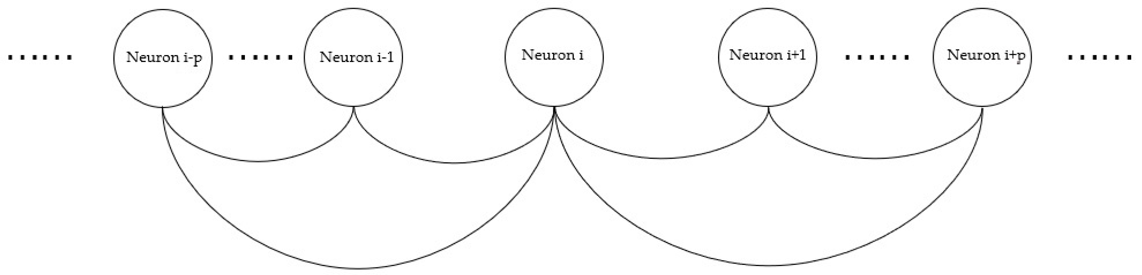
where and is the coupling strength of the network. If node i and node j are connected, . Each neuronal model is symmetrically coupled to its 2P nearest neighbors. It is important to note that implies that node j is coupled with node . The network structure is shown in Figure 1.
Then, the fractional-order neuronal ring network under electromagnetic radiation can be described as follows:
3. Synchronization Behavior of Two Fractional-Order Coupled Neuronal Models under Electromagnetic Radiation
As the simplest neuronal network, the synchronization behaviors of two coupled fractional-order neuronal models under electromagnetic radiation are researched first.
To prove that the two coupled fractional-order neuronal models can come into perfect synchronization, some lemmas and definitions are introduced as follows. The Mittag–Leffler function is defined by
Lemma 1.
[51] Let be a real continuous and differentiable vector function. Then, for all and , the following inequality holds:
Lemma 2.
Lemma 3.
Let,,. The error system is. According to (2), the error system can be described as
where
Theorem 1.
satisfyiesthe Lipschitz condition[54] if
Then, the two neuronal models can undergo global exponential synchronization.
Proof of Theorem 1.
Construct the Lyapunov function as . From Lemma 1, the Lyapunov function can be reduced to
From Lemma 2, , according to Lemma 3,
Therefore, as . When , we can conclude that the two neuronal modes can be in global exponential synchronization when under the appropriate coupling strength. □
The above condition is just sufficient, so it is necessary to investigate the details of the system’s synchronization behaviors and synchronization transition.
Fractional-order HR neuronal models under electromagnetic radiation were investigated in [27], and two neuronal models reached perfect synchronization through adaptive control. However, the synchronization behavior and synchronization transition induced by the fractional-order and other parameters are not reported in [27]. In this section, the synchronization behaviors and synchronization transitions induced by the fractional-order and the parameter are studied.
In this section, the similarity function is introduced to measure the synchronization of the system [7]. The model of the similarity function can be described as follows:
where stands for the time average.
Obviously, perfect synchronization can be observed when S is equal to 0, and the larger S is, the worse the synchronization.
The phase synchronization is introduced, and its synchronization degree is weaker than perfect synchronization. From the time of sampled time series across the Poincare section, the phase of the neuronal model can be calculated. The phase is calculated by [55]
The phase difference between two neuronal models is defined by
when the system is not in perfect and phase synchronization, it may be in bursting synchronization. Bursting synchronization means rhythm synchronization of slow variables, so bursting synchronization can be measured by the slow variable’s similarity function [55]. The model of the similarity function can be described as follows:
when is close to 0, the system reaches bursting synchronization.
3.1. Effect of Fractional-Order and Coupling Strength on the Synchronization under Electromagnetic Radiation
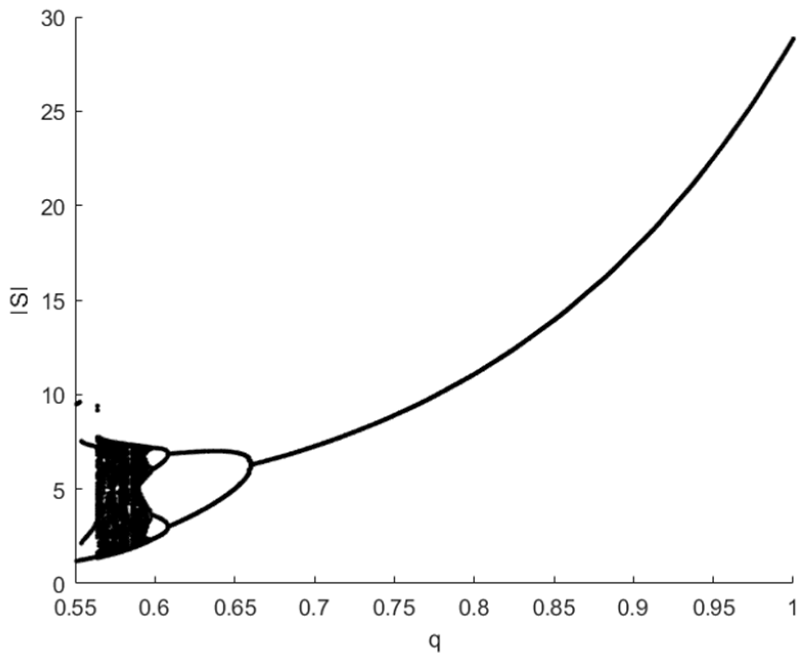
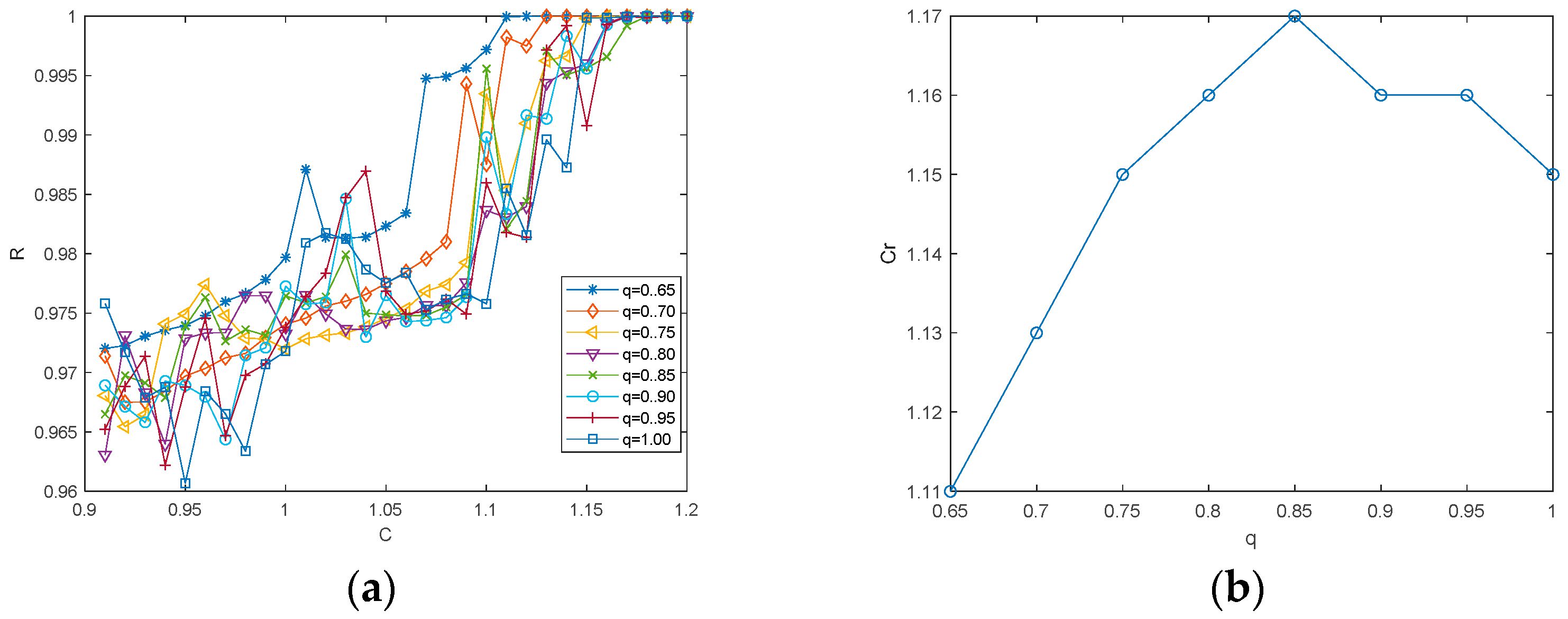
When , the fractional-order and parameter are varied in the regions and , the similarity function is shown in Figure 2, where the blue region with S equal to 0 denotes that the system is in perfect synchronization. As shown in Figure 2, when and the coupling strength is approximately 0.367, the similarity function undergoes a complex change, which means that the synchronous threshold of the coupling strength changes greatly. When , the synchronous threshold of the coupling strength decreases with increasing fractional order. When , the curves are shown in Figure 3. In [34], the threshold of the coupling strength only increases first and then decreases with increasing fractional-order.
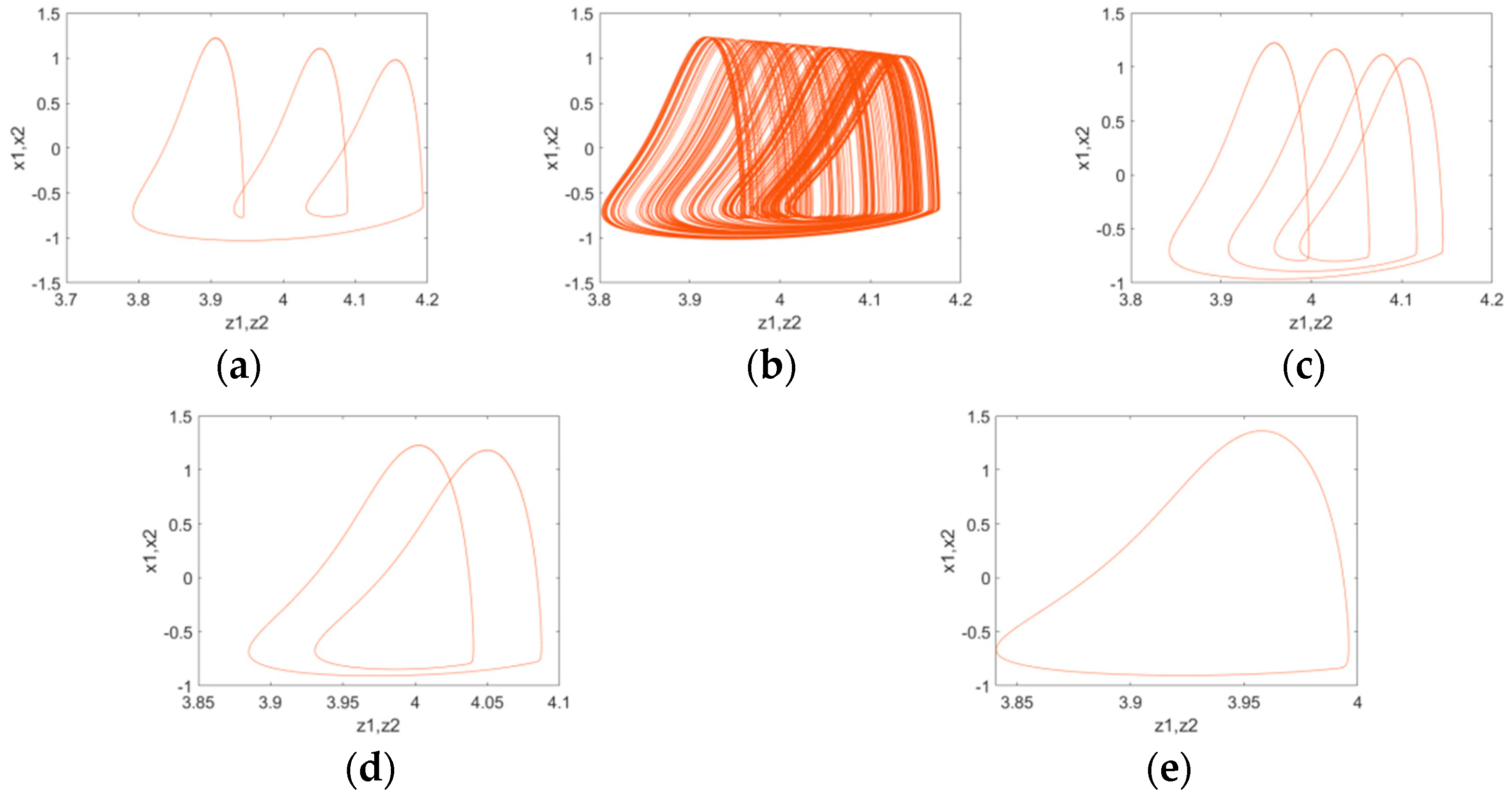
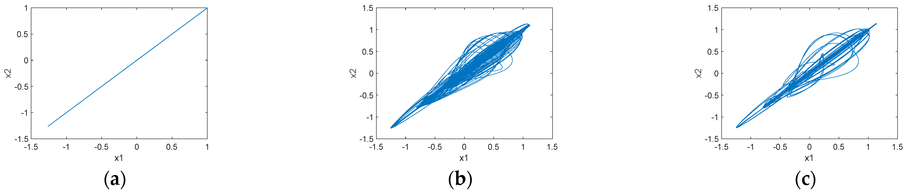
As shown in Figure 2, the similarity function has striking changes when , so the synchronization transition can be observed when . The synchronization transition when is taken as an example to observe the change in the synchronization mode. When , Figure 4a is the phase diagram of , and Figure 4b is the corresponding time series of and , so the system is in imperfect synchronization. As shown in Figure 4c,f, the system is in perfect synchronization when and because the phase plane is located on a three quadrant angular bisector. The system is in imperfect synchronization when , as shown in Figure 4d,e, and the neuronal models display spiking.
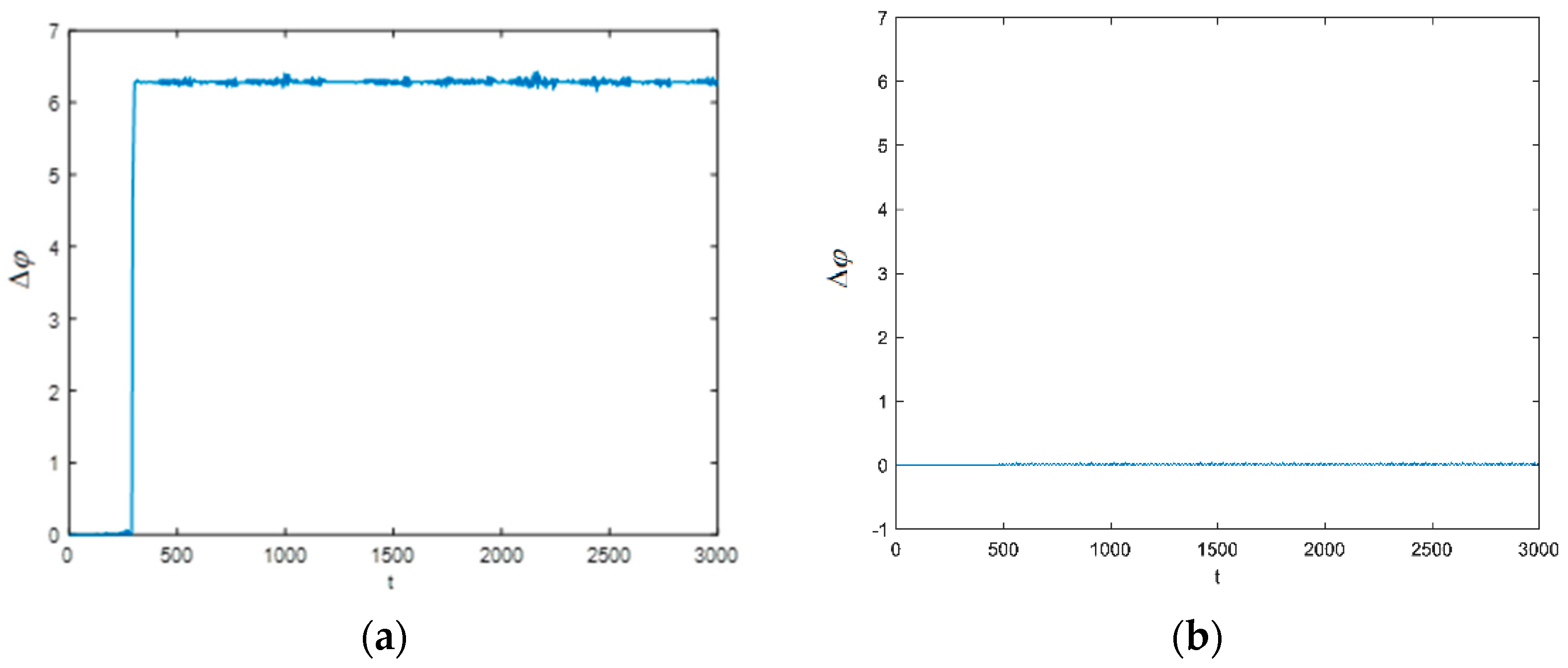
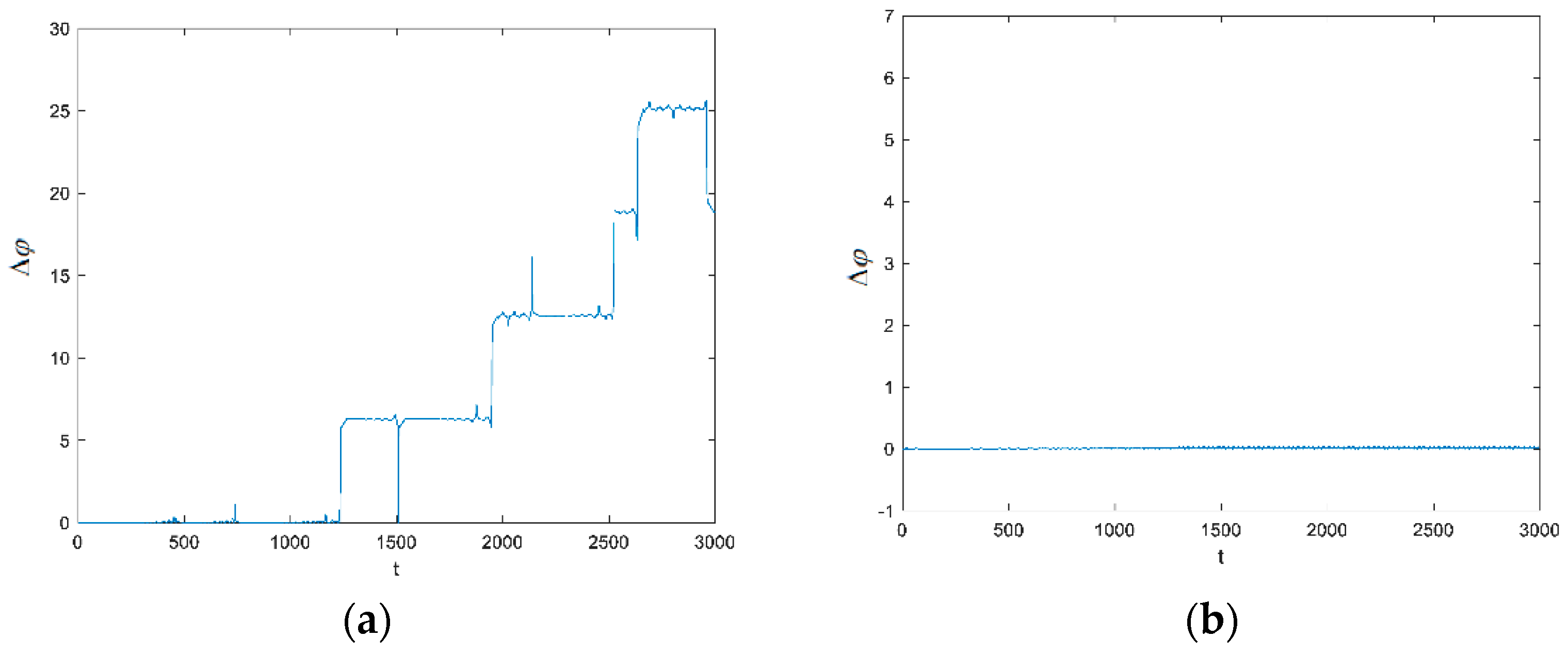
From Figure 4, when the two neuronal models are in imperfect synchronization, the phase difference is calculated as follows. As shown in Figure 5a, when the phase differences are always approximately 0 or , so the system achieves phase synchronization. From Figure 5b, the phase difference is approximately 0, so the system is also in phase synchronization when .
As mentioned above, the synchronization transition mode induced by fractional order is phase synchronization → perfect synchronization → phase synchronization → perfect synchronization. In [34], the synchronization transition near the threshold of coupling strength is perfect synchronization → phase synchronization → perfect synchronization. The transition mode in this paper is more complex than the coupled fractional-order neuronal models without electromagnetic radiation [34].
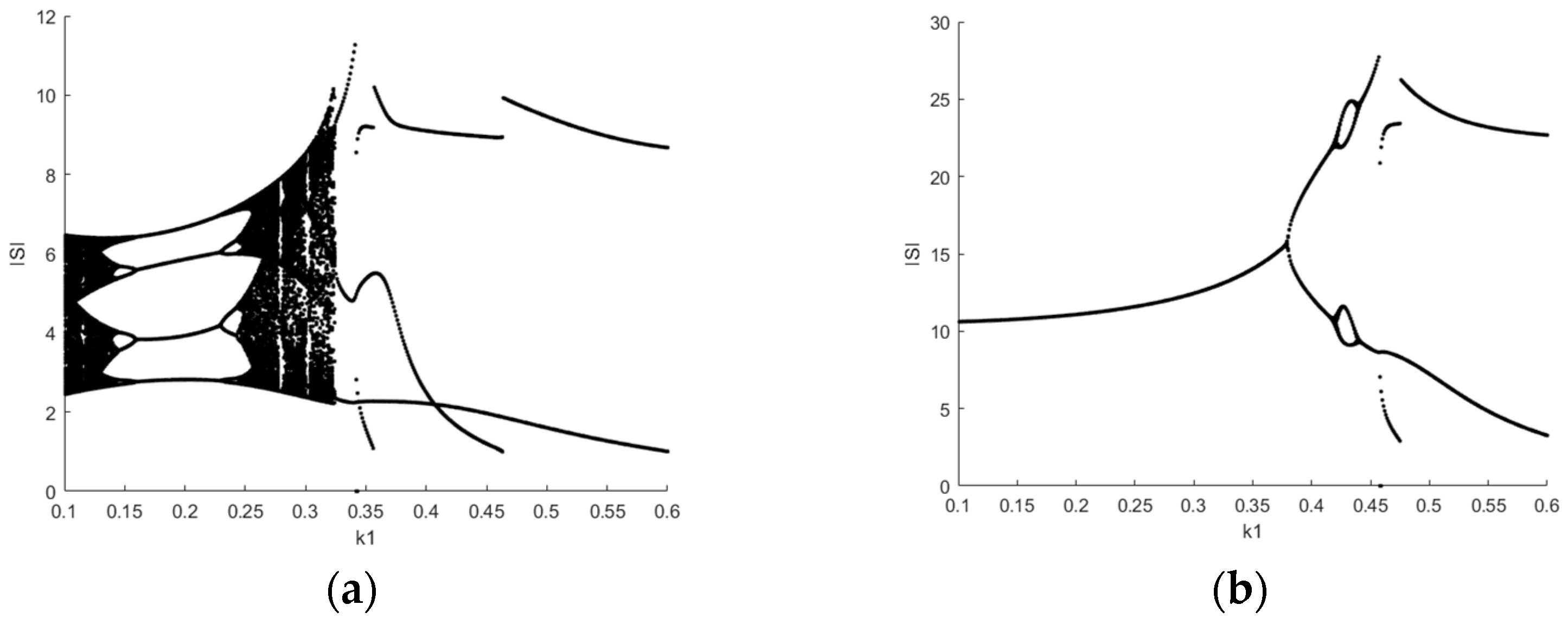
As shown in Figure 2, the two neuronal models are in perfect synchronization when and . Now, the ISI bifurcation of the first neuronal model for is shown in Figure 6. Double-period bifurcation exists when and with decreasing fractional-order. The system is in chaotic perfect synchronization when , but the system is in periodic perfect synchronization at other fractional orders. Figure 7 shows the phase diagram of when , , , , and for . The neuronal models display periodic-3 bursting, chaotic bursting, periodic-4 bursting, periodic-2 bursting, and spiking. The synchronization transition, which is perfect periodic-3 synchronization → perfect chaotic synchronization → perfect periodic-4 synchronization → perfect periodic-2 synchronization → perfect spiking synchronization, is observed. When the system is in perfect synchronization, the transition mode is also more complex than coupled neuronal models without electromagnetic radiation [34], because the synchronization transition is only perfect periodic-4 synchronization → perfect chaotic synchronization in [34]. The results show that when the system is in perfect synchronization, the fractional-order and electromagnetic radiation can also change the synchronization mode.
3.2. Effect of the Parameter and the Coupling Strength on the Synchronization under Different Fractional Order
In this section, the influence of parameter and coupling strength on the synchronization behaviors and the synchronization transition induced by is investigated. The similarity function, phase difference, and slow variable similarity function are also used to measure the synchronization degree of the system. From the analysis mentioned above, different fractional orders induce different dynamic behaviors. The influence of parameter and coupling strength on synchronization are studied under different fractional-orders.
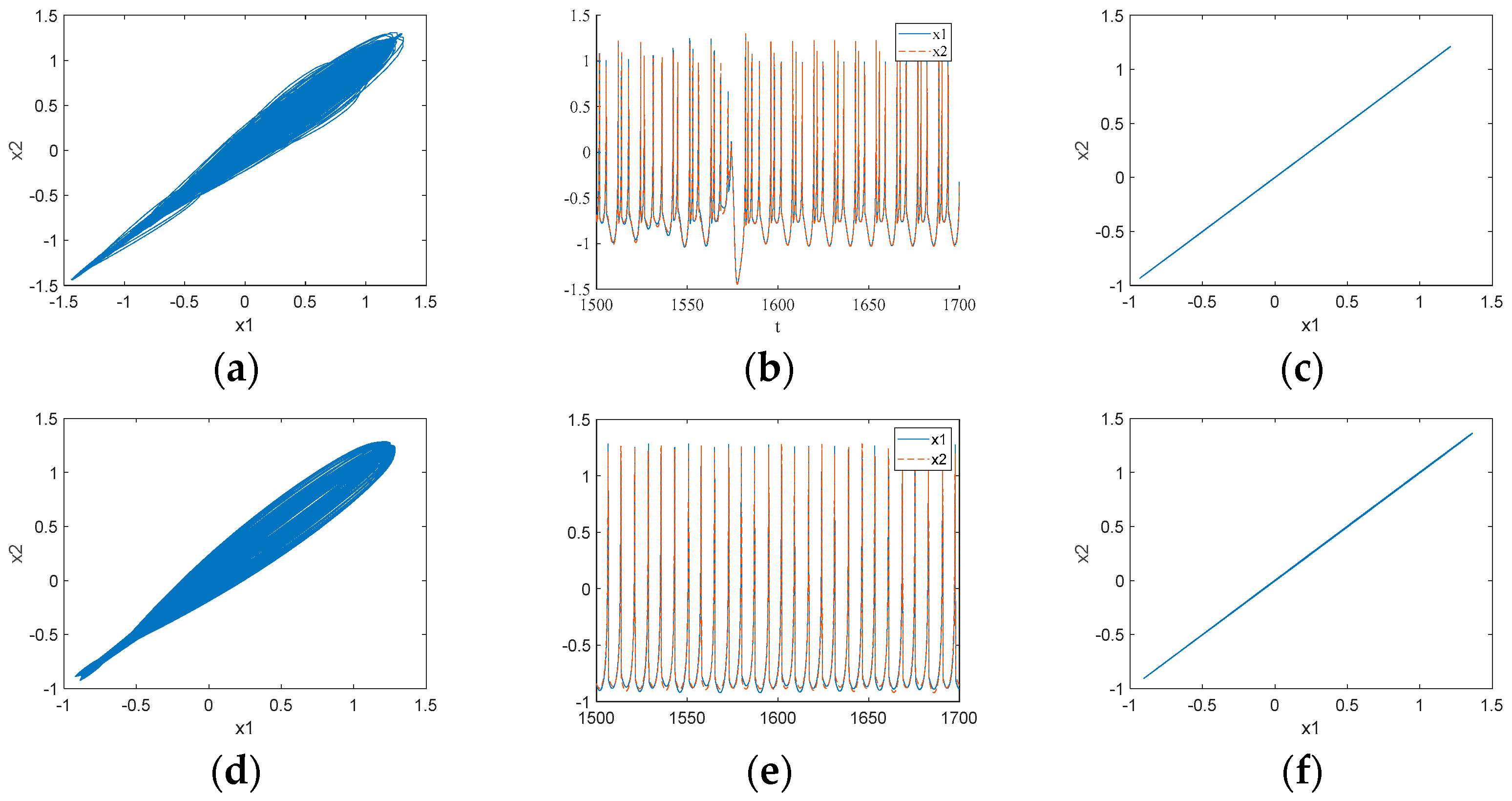
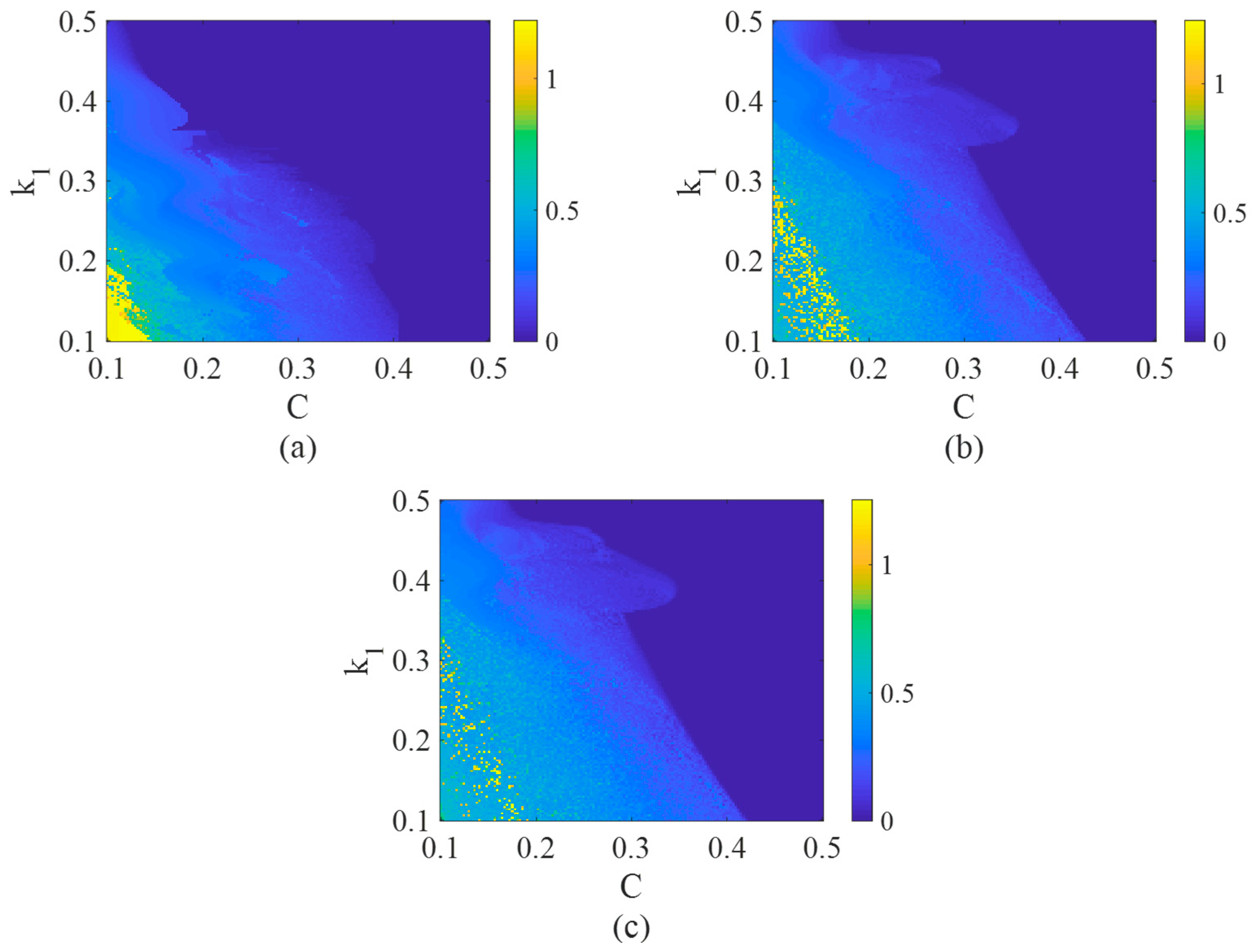
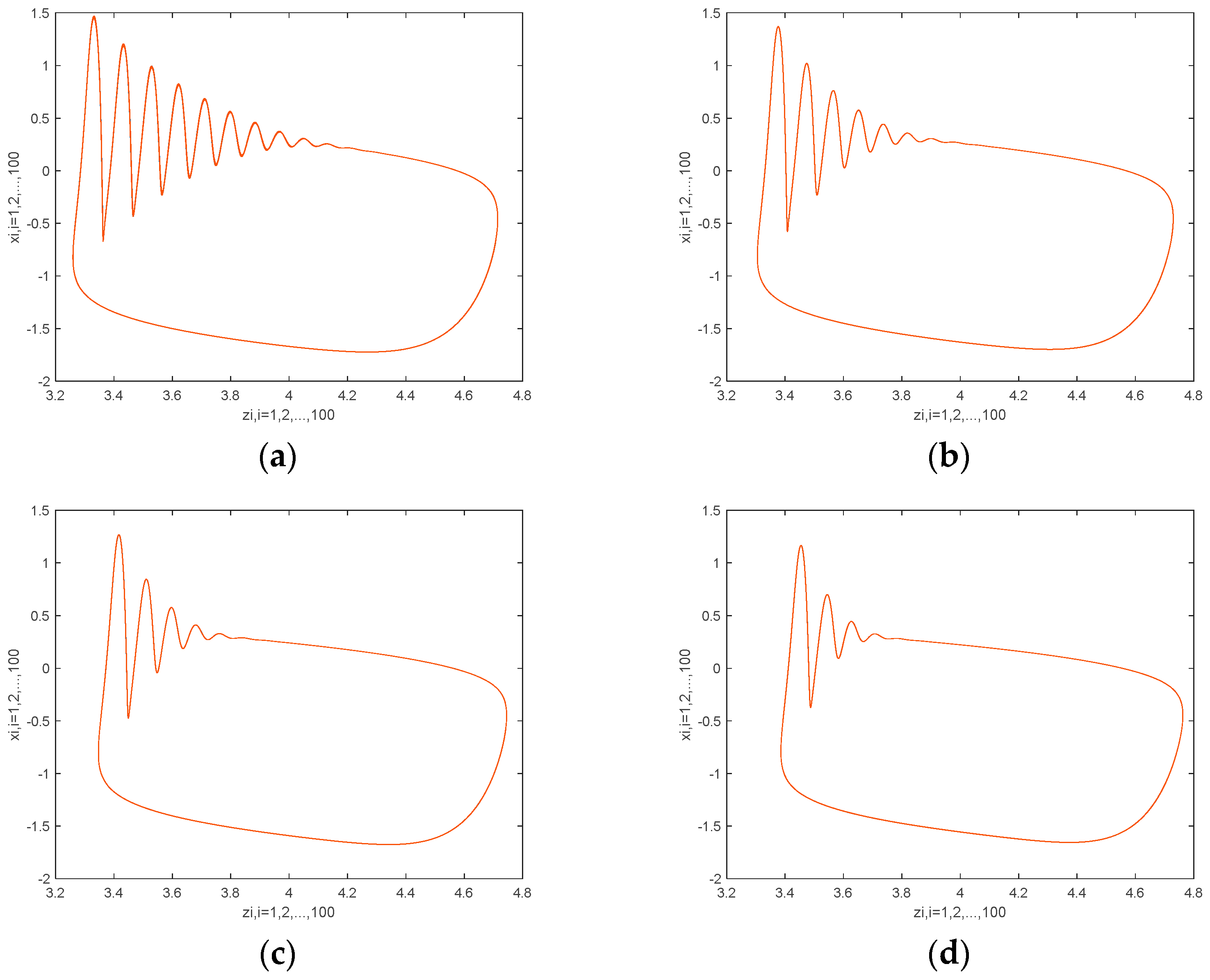
Therefore, the value of the similarity function in the plane for several fractional-order values is calculated, as shown in Figure 8. In this figure, the blue region where S equals 0 denotes a system in perfect synchronization. Generally, the conclusion that a large parameter and coupling strength can bring the system into perfect synchronization can be drawn. However, there is an exception: when and , a smaller can cause the system to be in perfect synchronization, but a larger cannot. As shown in Figure 9a, when , , the value of the similarity function decreases with increasing , and then when . However, with the sequential increase in , when . Then, when . To observe the above process more visually, the phase diagram and the corresponding time series are shown in Figure 9b–f when . As shown in Figure 9b,c, the phase diagram of and the corresponding time series of and show that the system is in imperfect synchronization when . From Figure 9d,f, the system is in perfect synchronization when and . The system is asynchronized when , as shown in Figure 9e.
The phase differences of and when and are plotted in Figure 10. We can conclude that the two neuronal models are in phase synchronization when , because the phase difference is small at approximately 0. The two neuronal models are not in phase synchronization when , but the phase is locked in some time periods, and the slow variable’s similarity function is calculated as , so the two neuronal models are in bursting synchronization. The synchronization transition induced by parameter , that is, bursting synchronization → perfect synchronization → phase synchronization → perfect synchronization, can be observed.
Figure 8 also shows that the range of synchronization when is the largest of the three values of . As shown in Figure 11, , the system is asynchronized when and , but the system is perfectly synchronized when .
If we change the parameter when the system is in perfect synchronization () for several values of , the synchronization mode also changes. The ISI bifurcation of the first neuronal model is plotted in Figure 12. As shown in Figure 12a, when and , the neuronal models display chaotic firing, but when and , the neuronal models display periodic firing. When , the parameter induces the transition of chaotic perfect synchronization and periodic perfect synchronization. As shown in Figure 12b, when , there is a double-period bifurcation when . can also induce the synchronization transition. Thus, the other kind of synchronization transition, in which the firing modes of the two perfect synchronization neuronal models are different, induced by is also observed.
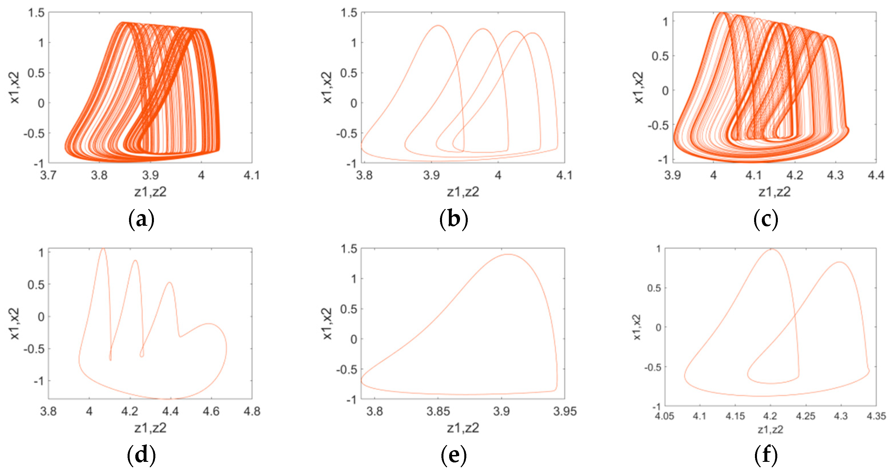
The phase diagrams of are shown in Figure 13 when . The synchronization transition induced by the parameter can be explained. Figure 13a,c show that the neuronal models display chaotic firing, so the system is in chaotic synchronization when and . From Figure 13b,d, the neuronal models display periodic-4 bursting and periodic-3 bursting, so the system is in periodic synchronization when and . The system is in periodic synchronization at all values of when , but the neuronal models display spiking firing and periodic-2 bursting when and , as shown in Figure 13e,f.
In [27], the effect of parameter on the synchronization was not investigated. In [46], when the neuronal model is an integer-order model, the synchronization mode is perfect spiking synchronization for all when . The conclusion can be summarized that parameter can induce the synchronization transition and that the synchronization behaviors are different when the fractional order varies. As shown in Figure 12 and Figure 13, a small fractional order, such as 0.6, can induce a more complex synchronization transition because when , the system has diverse synchronization modes such as chaotic synchronization and different kinds of periodic synchronization, but only periodic synchronization occurs when .
4. Synchronization Behavior of Fractional-Order Neuronal Ring Networks under Electromagnetic Radiation
In this paper, the synchronization factor is adopted to describe the synchronization of network. is given by [47]
where denotes the time averaging. The value of R is between 0 and 1, and it increases with decreasing average membrane potential errors. More precisely, perfect synchronization is expected when R is close to 1, and a nonsynchronization state may appear when R is close to 0.
The bursting synchronization of the neuronal network can be described by the slow variable’s synchronization factor . is given by
where denotes the time averaging. When is close to 1, the system reaches bursting synchronization.
4.1. Fractional-Order Neuronal Ring Network without Electromagnetic Radiation
To illustrate the diverse synchronization behaviors and synchronization transition modes, a fractional-order neuronal ring network without electromagnetic radiation is studied first.
The ring network consists of 100 nodes. Numerical simulation is provided for model (2) by utilizing the ADM method. As shown in Figure 14, the synchronous threshold of the coupling strength varies with the fractional-order. The change trend of the threshold first increases and then decreases, as shown in Figure 14b. In previous studies, for integer-order neuronal networks, the threshold of the coupling strength can change with other influencing factors [12,16], such as the structure of the network and time delay. In this paper, the fractional order is proven to be an influencing factor.
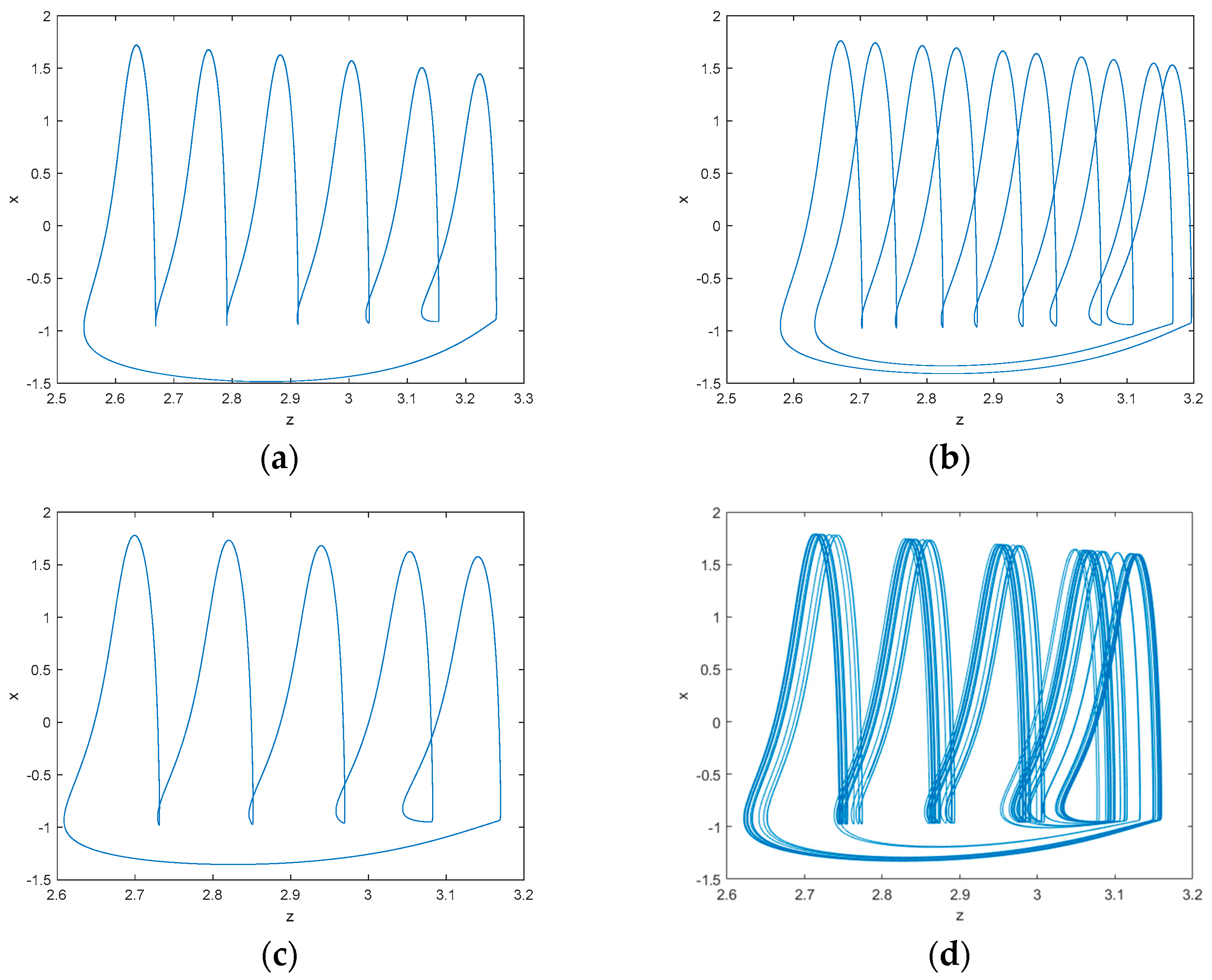
As shown in previous studies, for the integer-order neuronal network, a time-delay can induce the synchronization transition of the neuronal network [16,17]. In this paper, the results show that fractional-order not only makes the synchronous system become asynchronous, but it also changes the synchronization mode. When the neuronal network is in perfect synchronization, Figure 15 shows the phase diagram of when the fractional order is 0.65, 0.75, 0.85, and 0.95. The neurons display periodic-6 bursting, periodic-10 bursting, and periodic-5 bursting when , , and , as shown in Figure 15a–c, respectively. The network is in perfect periodic-6, perfect periodic-10 and perfect periodic-5 synchronization. When , as shown in Figure 15d, the neurons display chaotic bursting, so the network is in perfect chaotic synchronization. The fractional-order can induce the synchronization transition, which is perfect periodic-6 synchronization → perfect periodic-10 synchronization → perfect periodic-5 synchronization → perfect chaotic synchronization.
4.2. Fractional-Order Neuronal Network under Electromagnetic Radiation
In this section, the effect of some parameters on the synchronization behaviors of ring neuronal networks under electromagnetic radiation is investigated. In [37], the integer-order neuron’s firing activity is influenced by the parameter . In this paper, the firing activity is also influenced by the parameter apart from . In addition, in this paper, the results show that the fractional order cannot influence the neuronal models’ firing mode in the ring neuronal network under electromagnetic radiation. It is obviously different from the two coupled fractional-order neuronal models under electromagnetic radiation, single neuron and the ring neuronal network without electromagnetic radiation. Although the fractional-order cannot influence the neuronal firing mode, the fractional-order can influence the synchronization degree of the ring neuronal network under electromagnetic radiation under different conditions. For example, the ring neuronal network constructed by integer-order neuronal models is in perfect synchronization, but the perfect synchronization may be destroyed in the same conditions when the integer-order neuronal models are instead fractional-order neuronal models, or vice versa. Therefore, this paper focuses on the effects of parameters , and on the synchronization behaviors and synchronization transition of ring neuronal networks constructed by fractional-order neuronal models.
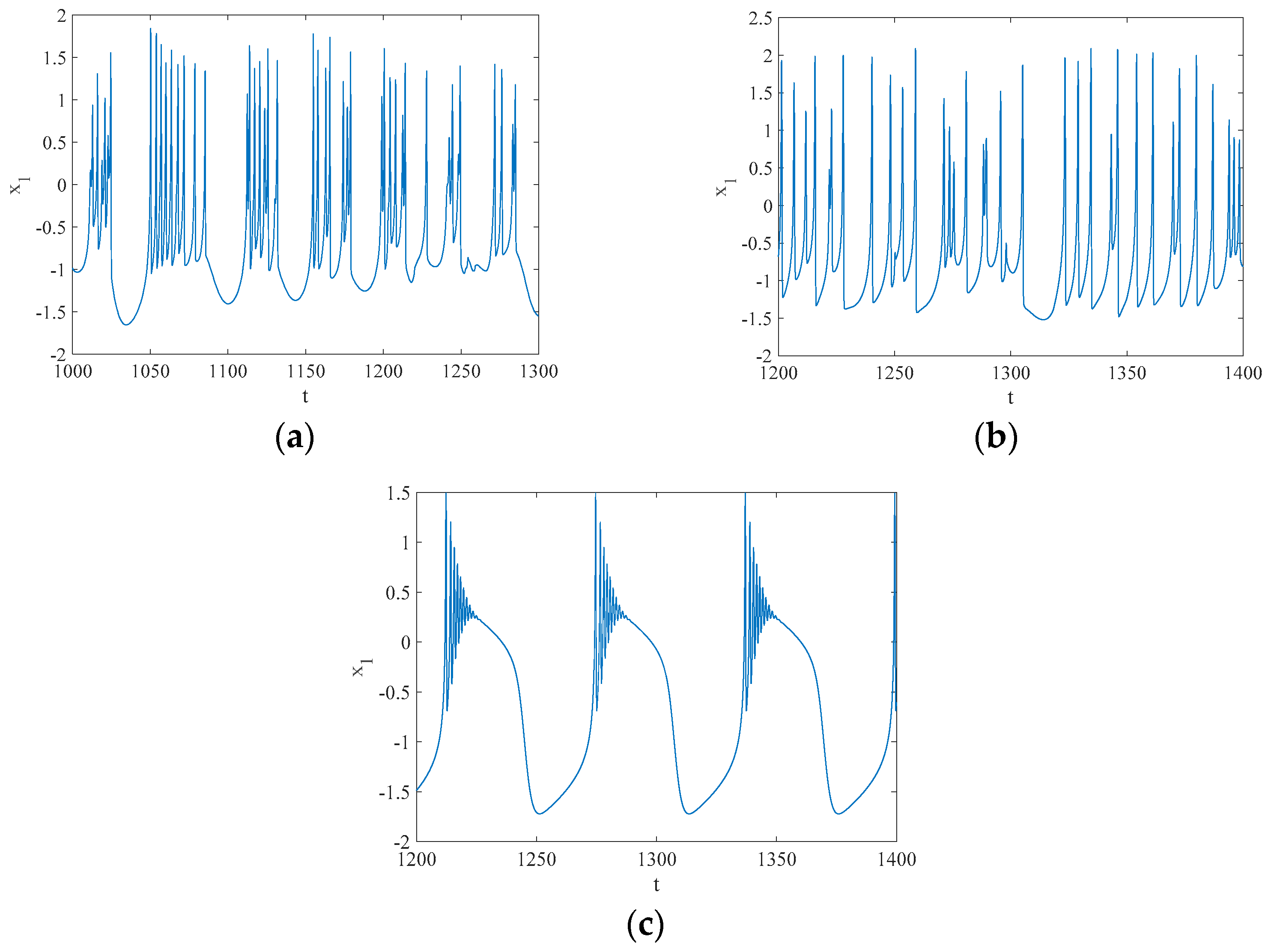
The firing mode with different parameter when is plotted in Figure 16, and the other parameters are set as mentioned in Section 1. Figure 16 shows the firing mode of the first neuron when the parameter is different. From the numerical simulations, we can find that the neuronal models display chaotic bursting, spiking firing, and periodic bursting when , , and . In this section, the synchronization behaviors in the three regions of are studied numerically.
4.2.1. Synchronization Behavior of the Neuronal Network When
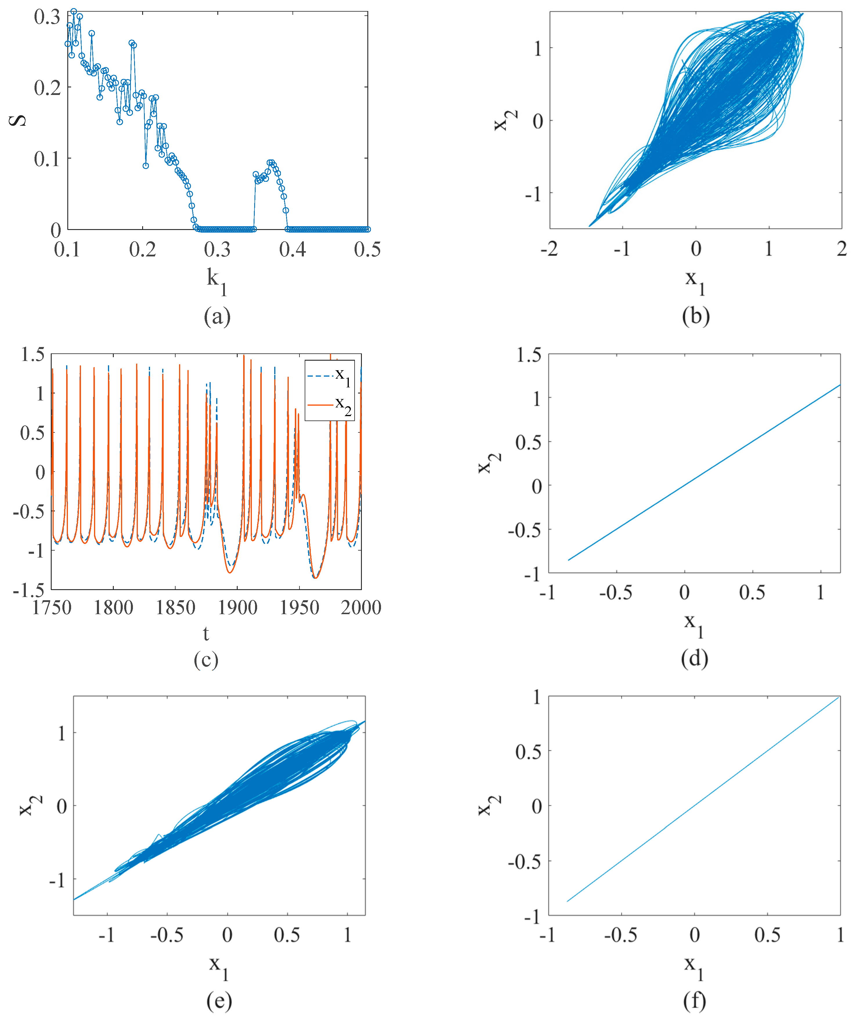
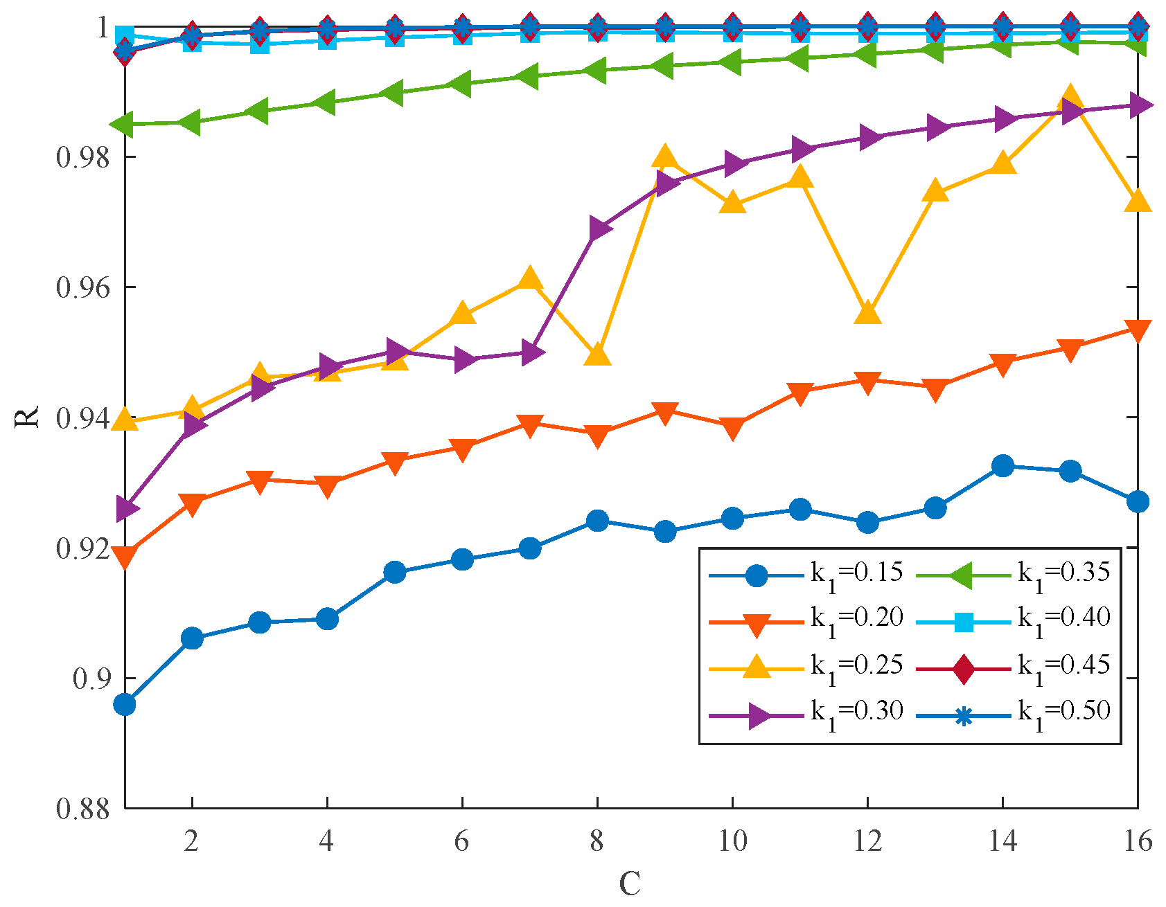
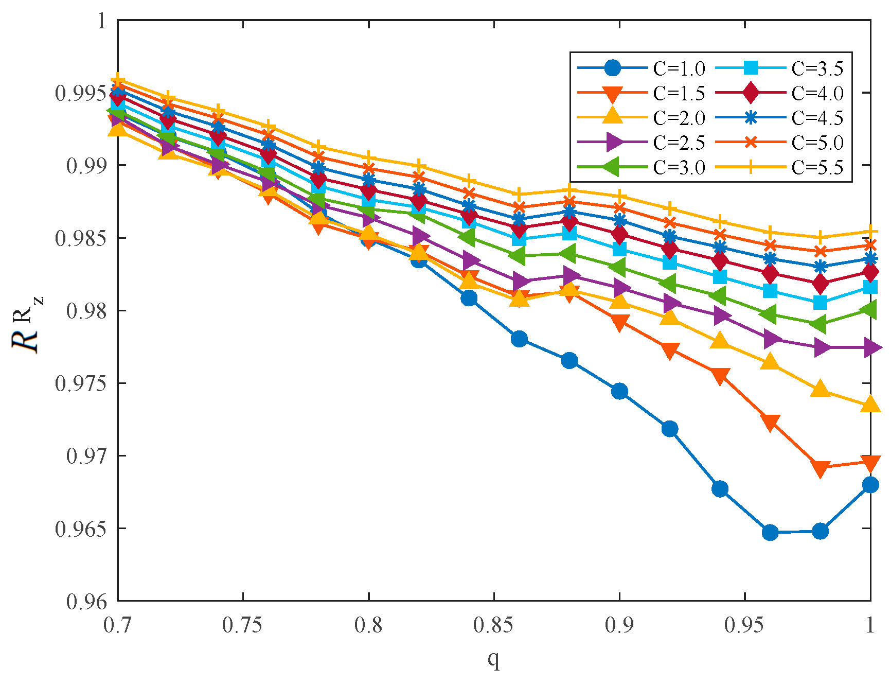
In this part, the parameter is set as an example. The curves of when for different are shown in Figure 17. From Figure 17, we find the effects of parameter and coupling strength on synchronization behaviors. The synchronization factor increases with increasing coupling strength and . When , plays a dominant role in the network synchronization, because the network cannot reach perfect synchronization when and the coupling strength ranges from 1 to 16. The state of the network can be transformed from asynchronization to perfect synchronization with a minor change in when .
To observe the effect of fractional order, is set as 0.35. Fractional order cannot influence the neuronal models’ firing mode, but it can change the synchronization degree. Figure 18 shows the curves for different coupling strengths. We can conclude that the increase in fractional order weakens the synchronization of the neuronal network. The synchronization is robust against alterations of coupling strength when fractional order is small. When the fractional order is 0.7, the difference in the synchronization factor between coupling strengths 1 and 5.5 is only 0.05, but when the fractional-order is 1, the difference becomes 0.2.
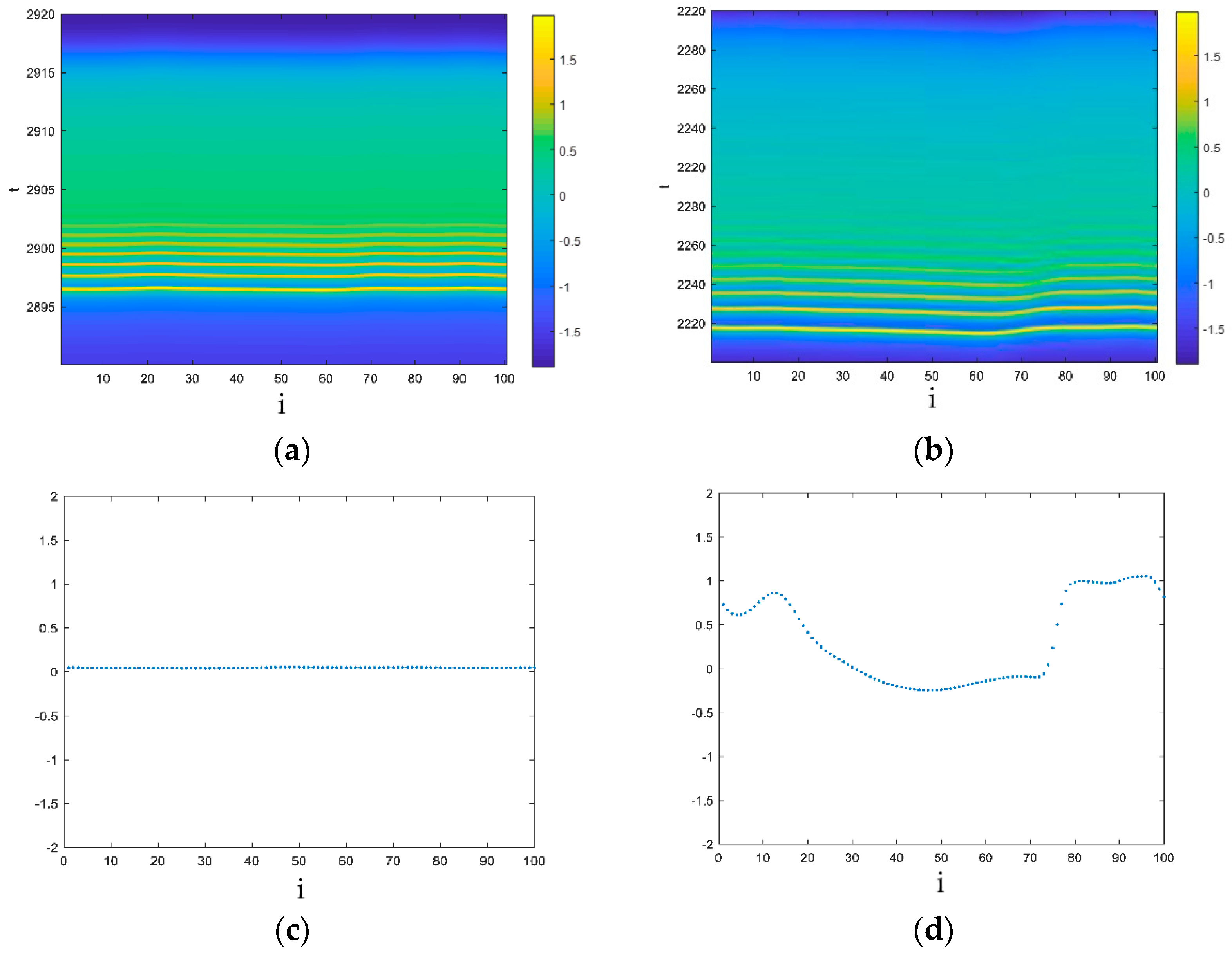
Figure 19 shows the neuronal network’s spatiotemporal patterns and corresponding snapshots when . It is concluded that the strength of synchronization is higher when the fractional order is 0.7 than when the fractional order is 0.98. When , the are uniformly distributed values, so the network is in nearly perfect synchronization. When , the are disorderly. However, the slow variable’s synchronization factor is calculated as 0.99, so the network is in bursting synchronization. The fractional-order can also induce the transition of perfect synchronization and bursting synchronization when the ring network is under electromagnetic radiation.
In addition, can also induce synchronization transition; that is, the firing mode of neuronal models changes for different when the network is in perfect synchronization. The parameters are set as and the neuronal network is in perfect synchronization. Figure 20 shows the phase diagram of when . As shown in Figure 20, a neuronal model in the network displays periodic-10 bursting, periodic-7 bursting, periodic-5 bursting, and periodic-4 bursting when . The number of spikes in one bursting decreases with increasing , so the synchronization mode varies with . The synchronization transition induced by , which is perfect periodic-10 synchronization → perfect periodic-7 synchronization → perfect periodic-5 synchronization → perfect periodic-4 synchronization, is observed.
4.2.2. Synchronization Behavior of the Neuronal Network When
In this part, the parameter is set as an example. The synchronization is different from the above analysis. As shown in Figure 21, the synchronization factor also increases with increasing coupling strength and , but we can conclude that it is difficult to reach perfect synchronization. The coupling strength ranges from 1 to 16, and the synchronization factor just reaches approximately 0.3.
The neuronal network’s spatiotemporal patterns and corresponding snapshots at when are shown in Figure 22. It is found that the are disorderly when the coupling strength is 1 and 16. The degree of synchronization is higher when the coupling strength is 16 than when the coupling strength is 1, but they are not synchronized. After calculating the slow variable’s synchronization factor, the network is not in bursting synchronization. This part of the view is different from the case of the network without electromagnetic radiation, as shown in Figure 15d. Under the same fractional-order and coupling strength, the network can be in perfect synchronization.
4.2.3. Synchronization Behavior of the Neuronal Network When
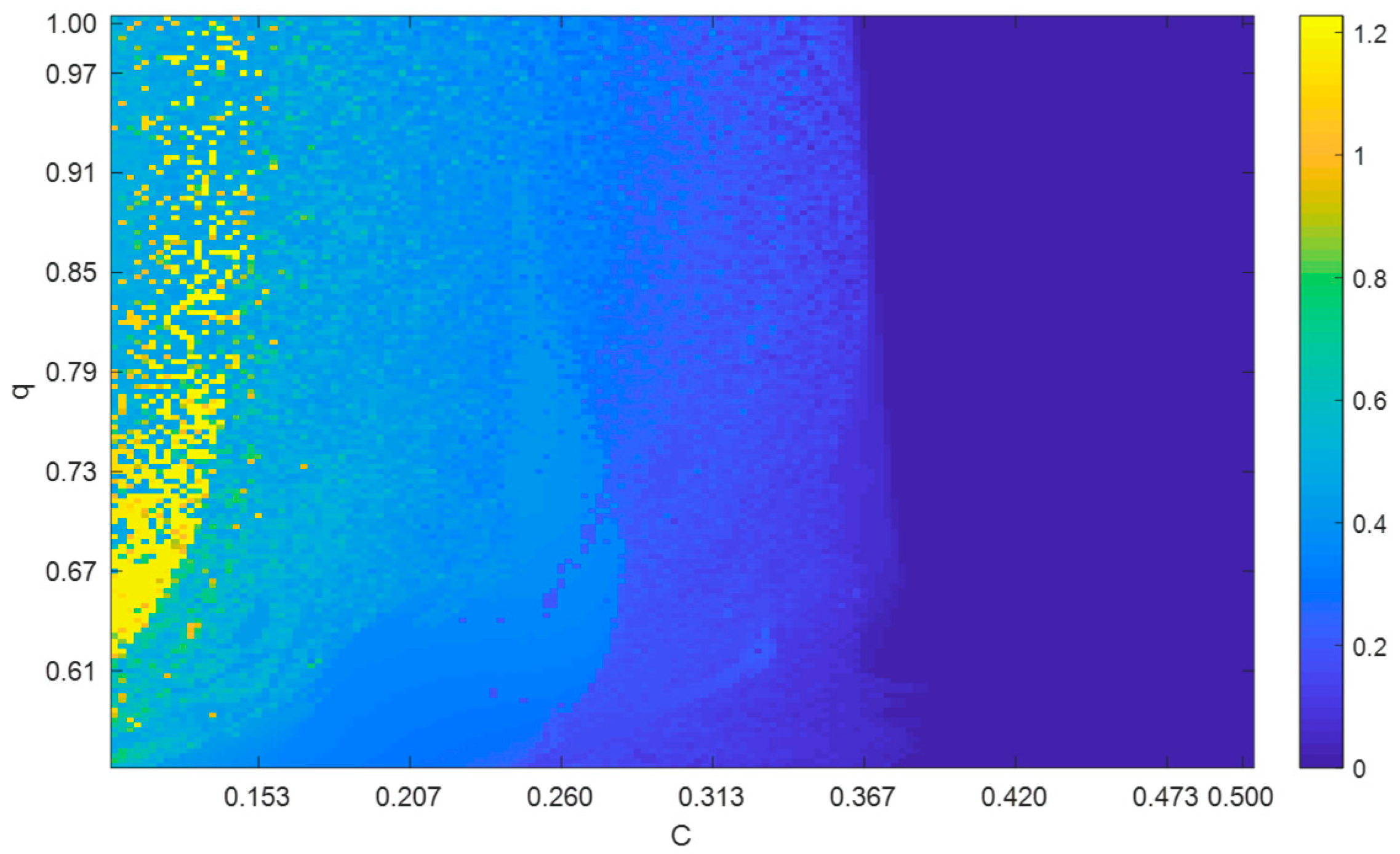
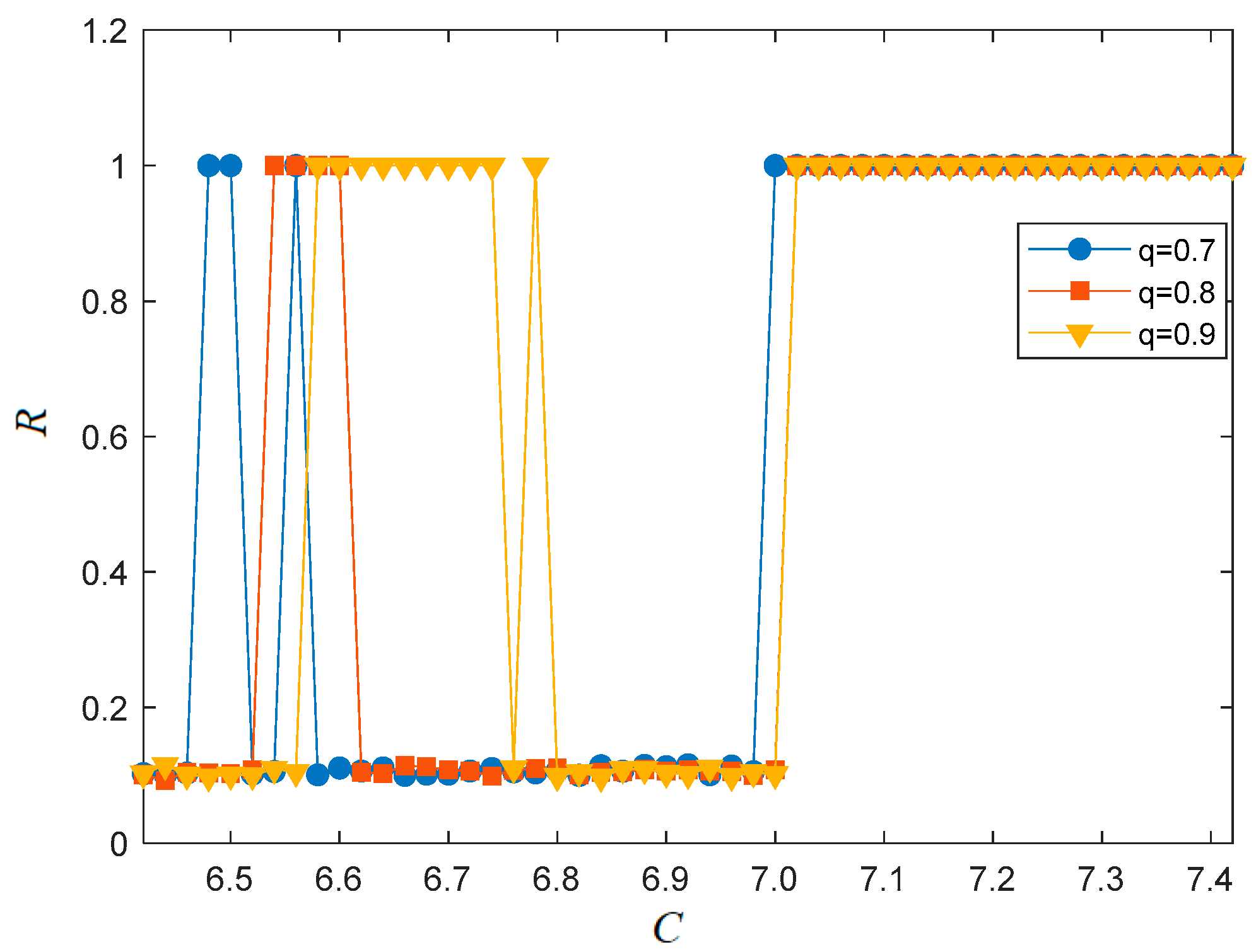
In this section, the parameter is set as an example. Some novel phenomena are observed. The curves when for different fractional-orders are plotted in Figure 23. We find that the network is in perfect synchronization when , but the neuronal models’ dynamic behaviors are different when for different fractional orders. In addition, the transition of synchronization and asynchronization is abrupt when the fractional-order and coupling strength change slightly. The synchronization factor changes from 0.1 to 1 directly. This phenomenon is not found in previous studies.
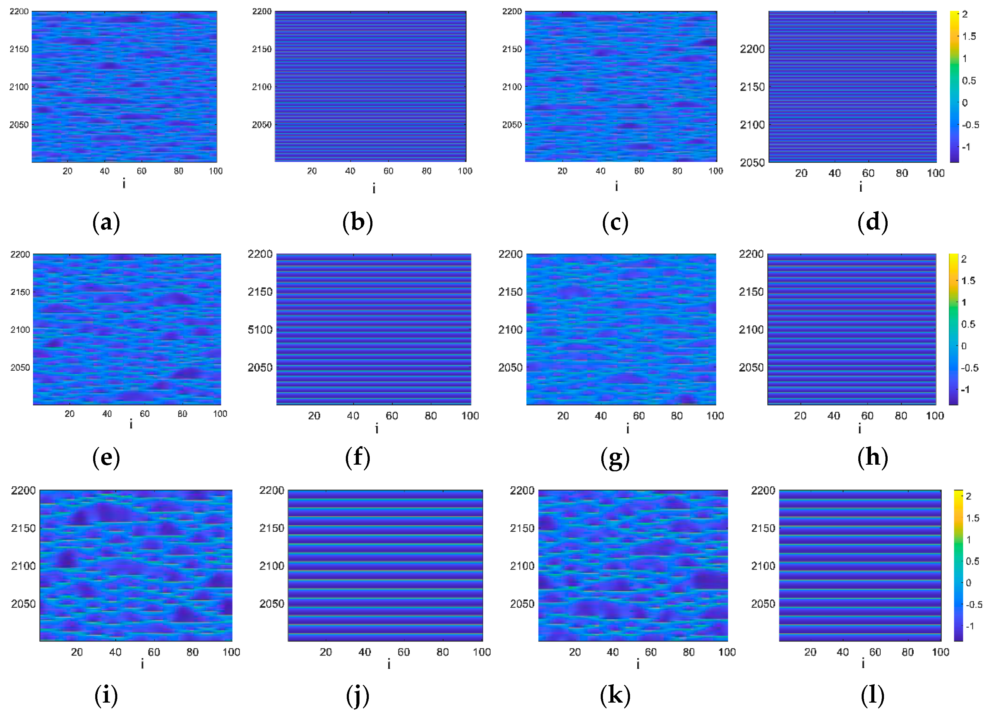
Figure 24 shows the neuronal network spatiotemporal patterns at different fractional orders and coupling strengths. As shown in Figure 24, for each fractional order, the network undergoes several sudden transitions of asynchronization and perfect synchronization with the variation in coupling strength. The dynamic behavior of neuronal models in the network is different at different fractional-orders and coupling strengths. When , the network is asynchronized at and , but the network is perfectly synchronized at . When , the network is in perfect synchronization at , but the network is in asynchronization at and . When , fractional-order can also induce a synchronization transition. We can find that the larger the fractional-order is, the larger the range of asynchronization, as shown in Figure 23. From the value of the slow variable’s synchronization factor when the network is not in perfect synchronization, the network cannot obtain bursting synchronization. In the neuronal network without electromagnetic radiation, we could not find the abrupt changes in the synchronization factor and synchronization behaviors.
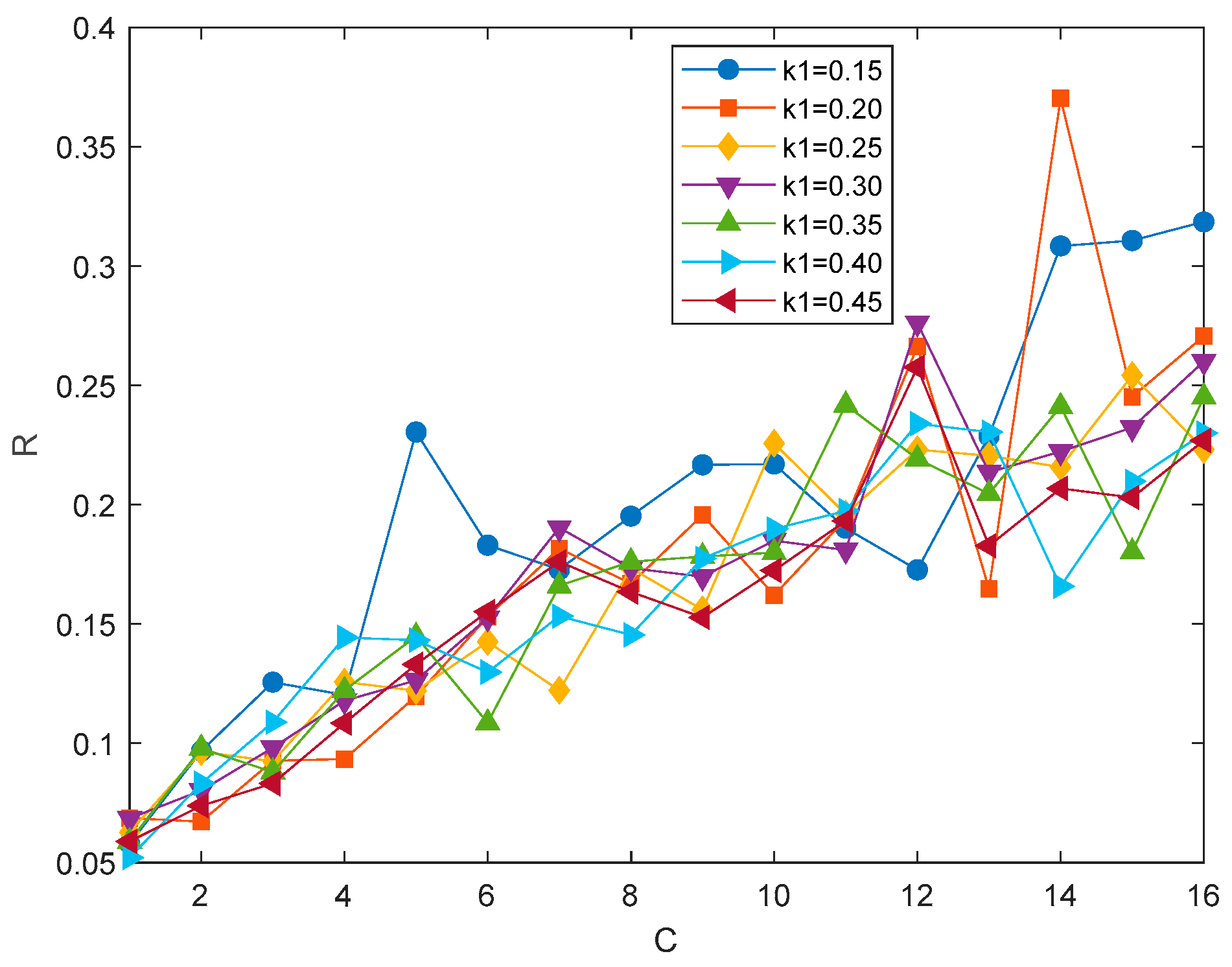
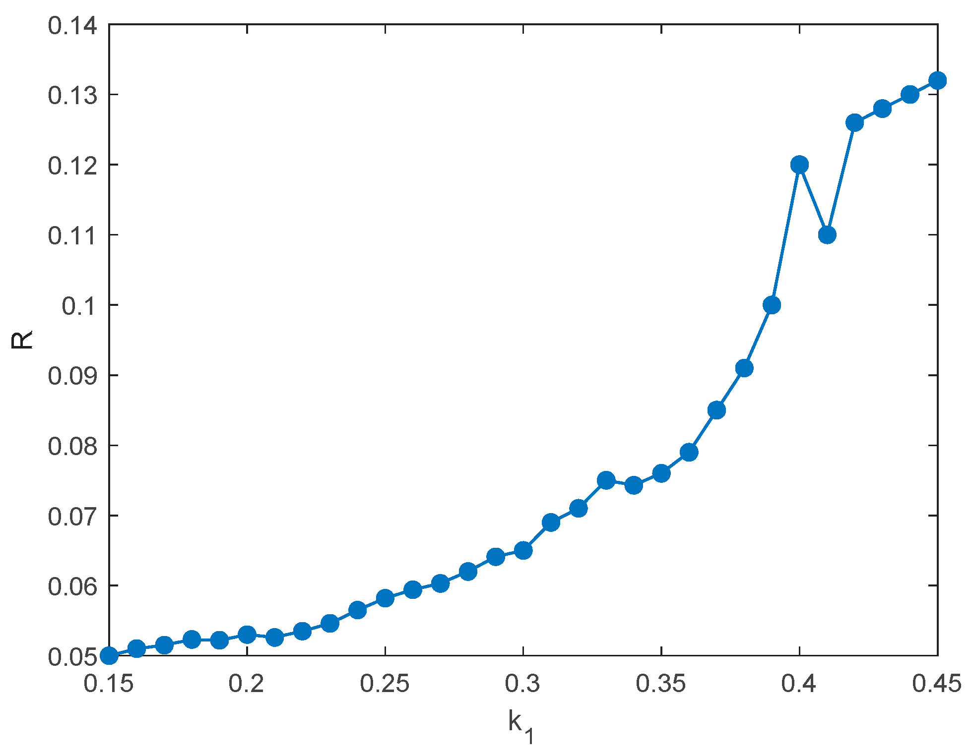
For the influence of , as shown in Figure 25, the synchronization degree increases when increases, but the network has difficulty obtaining perfect synchronization. The parameters are set as , .
5. Conclusions
This paper investigates the synchronization behaviors and synchronization transitions of fractional-order neuronal networks under electromagnetic radiation.
- (1)
- For the two coupled neuronal models under electromagnetic radiation:
- (a)
- With increasing fractional-order, the synchronous threshold of the coupling strength fluctuates first, then increases and finally decreases (in [34] (without electromagnetic radiation), the threshold of coupling strength only increases first and then decreases with increasing fractional-order).
- (b)
- The synchronization transitions of the coupled fractional-order neuronal models, which contain bursting synchronization, perfect synchronization, and phase synchronization, are observed when the fractional-order or parameter changes.
- (c)
- In addition, when the two coupled neuronal models are in perfect synchronization, the transition of perfect chaotic synchronization and perfect periodic synchronization is observed when changing the fractional order or parameter . From the ISI bifurcation diagram in Figure 12, when , the system has more diverse synchronization modes, which are perfect chaotic synchronization, perfect periodic-6 synchronization, perfect periodic-4 synchronization, perfect periodic-3 synchronization, and perfect periodic-2 synchronization when the value of is different. However, when , only perfect periodic-2 → spiking synchronization occurs with increasing . Compared with [28], more diverse synchronization behaviors and synchronization transition induced by fractional order and other parameters were found, like the synchronization transition of phase synchronization, perfect synchronization and bursting synchronization, and our work shows more details of the synchronization behaviors of coupled fractional-order neuronal networks under electromagnetic radiation.
- (2)
- For the ring network constructed by fractional-order HR models without electromagnetic radiation:
- (3)
- For the same ring network under electromagnetic radiation.
- Different from the results of [37] in which only the parameter changes the firing activities of neuronal models in the network, this paper focuses on the influence of the parameters , and fractional-order on the synchronization behaviors and synchronization transitions. Obviously different from the integer-order neuronal network and the fractional-order neuronal network without electromagnetic radiation, the fractional orders cannot change the firing activity of a single neuronal model in the fractional-order neuronal network with electromagnetic radiation. However, can influence the synchronization degree of ring fractional-order neuronal networks.
- (a)
- When , the synchronization degree decreases with increasing fractional-order. The parameter can induce the synchronization transition of perfect periodic-10 synchronization, perfect periodic-7 synchronization, perfect periodic-5 synchronization, and perfect periodic-4 synchronization.
- (b)
- When , it is difficult for the network to reach synchronization, and the fractional order has difficulty changing the synchronization degree.
- (c)
- In particular, when , the network has a sudden transition of asynchronization and perfect synchronization. The synchronization factor goes suddenly from 0.1 to 1. The larger the fractional order is, the larger the range of asynchronization is. The synchronization degree increases with increasing .
Author Contributions
Conceptualization, X.Y. and G.Z.; methodology, X.Y.; validation, X.Y.; data curation, X.Y.; writing—original draft preparation, X.Y.; writing—review and editing, G.Z. and D.W.; visualization, X.Y.; supervision, X.L. All authors have read and agreed to the published version of the manuscript.
Funding
This research received no external funding.
Institutional Review Board Statement
Not applicable.
Informed Consent Statement
Not applicable.
Data Availability Statement
The data used to support the findings of this study are included within the article, and other data used can be obtained from the corresponding author upon request.
Conflicts of Interest
The authors declare no conflict of interest.
References
- Hodgkin, A.L.; Huxley, A.F. A quantitative description of membrane current and its application to conduction and excitation in nerve. J. Physiol. 1952, 117, 500–544. [Google Scholar] [CrossRef] [PubMed]
- FitzHugh, R. Impulses and physiological states in theoretical models of nerve membrane. Biophys. J. 1961, 1, 445–466. [Google Scholar] [CrossRef] [Green Version]
- Morris, C.; Lecar, H. Voltage oscillations in the barnacle giant muscle fiber. Biophys. J. 1981, 35, 193–213. [Google Scholar] [CrossRef] [Green Version]
- Hindmarsh, J.L.; Rose, R.M. A model of neuronal bursting using three coupled first order differential equations. Soc. Lond. B Biol. 1984, 221, 87–102. [Google Scholar]
- Levy, R.; Hutchison, W.D.; Lozano, A.M.; Dostrovsky, J.O. High-frequency synchronization of neuronal activity in the subthalamic nucleus of Parkinsonian Patients with Limb Tremor. J. Neurosci. 2000, 20, 7766–7775. [Google Scholar] [CrossRef] [Green Version]
- Ayala, G.F.; Dichter, M.R.; Gumnit, J.; Matsumoto, H.; Spencer, W.A. Genesis of epileptic interictal spikes. New knowledge of cortical feedback systems suggests a neurophysiological explanation of brief paroxysms. Brain Res. 1973, 52, 1–17. [Google Scholar] [CrossRef]
- Wang, Q.Y.; Lu, Q.S.; Wang, H.X. Transition to complete synchronization via near-synchronization in two coupled chaotic neurons. Chin. Phys. 2005, 14, 2189–2195. [Google Scholar]
- Wang, Q.Y.; Duan, Z.S.; Perc, M.; Chen, G.R. Synchronization transitions on small-world neuronal networks: Effects of information transmission delay and rewiring probability. Europhys. Lett. 2008, 83, 4404–4410. [Google Scholar] [CrossRef] [Green Version]
- Xu, F.; Zhang, J.; Fang, T. Synchronous dynamics in neural system coupled with memristive synapse. Nonlinear Dyn. 2018, 92, 1395–1402. [Google Scholar] [CrossRef]
- Ma, J.; Mi, L.; Zhou, P.; Xu, Y.; Hayat, T. Phase synchronization between two neurons induced by coupling of electromagnetic field. Appl. Math. Comput. 2017, 307, 321–328. [Google Scholar] [CrossRef]
- Parastesh, F.; Azarnoush, H.; Jafari, S.; Hatef, B.; Perc, M.; Repnik, R. Synchronizability of two neurons with switching in the coupling. Appl. Math. Comput. 2019, 350, 217–223. [Google Scholar] [CrossRef]
- Bandyopadhyay, A.; Kar, S. Impact of network structure on synchronization of Hindmarsh–Rose neurons coupled in structured network. Appl. Math. Comput. 2018, 333, 194–212. [Google Scholar] [CrossRef]
- Parastesh, F.; Chen, C.Y.; Azarnoush, H.; Jafari, S.; Hatef, B. Synchronization patterns in a blinking multilayer neuronal network. Eur. Phys. J. Spec. Top. 2019, 228, 2465–2474. [Google Scholar] [CrossRef]
- Budzinski, R.C.; Boaretto, B.R.R.; Prado, T.L.; Viana, R.L.; Lopes, S.R. Synchronous patterns and intermittency in a network induced by the rewiring of connections and coupling. Chaos 2019, 29, 123132. [Google Scholar] [CrossRef] [PubMed]
- Perez, T.; Garcia, G.C.; Eguiluz, V.M.; Vicente, R.; Pipa, G.; Mirasso, C. Effect of the Topology and Delayed Interactions in Neuronal Networks Synchronization. PLoS ONE 2011, 6, e19900. [Google Scholar] [CrossRef] [Green Version]
- Sun, X.J.; Perc, M.; Kurths, J. Effects of partial time delays on phase synchronization in Watts-Strogatz small-world neuronal networks. Chaos 2017, 27, 053113. [Google Scholar] [CrossRef] [PubMed]
- Sun, X.J.; Li, G.F. Synchronization transitions induced by partial time delay in an excitatory-inhibitory coupled neuronal network. Nonlinear Dyn. 2017, 89, 2509–2520. [Google Scholar] [CrossRef]
- Bao, B.C.; Yang, Q.F.; Zhu, D.; Zhang, Y.Z.; Xu, Q.; Chen, M. Initial-induced coexisting and synchronous firing activities in memristor synapse-coupled Morris-Lecar bi-neuron network. Nonlinear Dyn. 2020, 99, 2339–2354. [Google Scholar] [CrossRef]
- He, S.; Natiq, H.; Banerjee, S.; Sun, K. Complexity and Chimera States in a Network of Fractional-Order Laser Systems. Symmetry 2021, 13, 341. [Google Scholar] [CrossRef]
- Ge, M.Y.; Jia, Y.; Xu, Y.; Lu, L.L.; Wang, H.W.; Zhao, Y.J. Wave propagation and synchronization induced by chemical autapse in chain Hindmarsh-Rose neural network. Appl. Math. Comput. 2019, 352, 136–145. [Google Scholar] [CrossRef]
- Shi, J.C.; Luo, M.; Huang, C.S. Dependence of synchronization transitions on mean field approach in two-way coupled neural system. Indian J. Phys. 2018, 92, 1009–1016. [Google Scholar] [CrossRef]
- Ge, M.Y.; Jia, Y.; Kirunda, J.B.; Xu, Y.; Shen, J.; Lu, L.L. Propagation of firing rate by synchronization in a feed-forward multilayer Hindmarsh-Rose neural network. Neurocomputing 2018, 320, 60–68. [Google Scholar] [CrossRef]
- Gopal, R.; Chandrasekar, V.K.; Venkatesan, A.; Lakshmanan, M. Observation and characterization of chimera states in coupled dynamical systems with nonlocal coupling. Phys. Rev. E 2014, 89, 052914. [Google Scholar] [CrossRef] [PubMed] [Green Version]
- Kim, S.Y.; Lim, W. Burst synchronization in a scale-free neuronal network with inhibitory spike-timing-dependent plasticity. Cogn. Neurodyn. 2019, 13, 53–73. [Google Scholar] [CrossRef] [PubMed]
- Dong, J.; Zhang, G.J.; Xie, Y.; Yao, H.; Wang, J. Dynamic behavior analysis of fractional-order Hindmarsh-Rose neuronal model. Cogn. Neurodyn. 2014, 8, 167–175. [Google Scholar]
- Giresse, T.A.; Crepin, K.T.; Martin, T. Generalized synchronization of the extended Hindmarsh-Rose neuronal model with fractional order derivative. Chaos Soliton. Fract. 2019, 118, 311–319. [Google Scholar] [CrossRef]
- Meng, F.Q.; Zeng, X.Q.; Wang, Z.L.; Wang, X.J. Adaptive Synchronization of Fractional-Order Coupled Neurons Under Electromagnetic Radiation. Int. J. Bifurcat. Chaos 2020, 30, 2050044. [Google Scholar] [CrossRef]
- Meng, F.Q.; Zeng, X.Q.; Wang, Z.L. Dynamical behavior and synchronization in time-delay fractional-order coupled neurons under electromagnetic radiation. Nonlinear Dyn. 2019, 95, 1615–1625. [Google Scholar] [CrossRef]
- Lundstrom, B.N.; Higgs, M.H.; Spain, W.J. Fractional differentiation by neocortical pyramidal neurons. Nat. Neurosci. 2008, 1, 1335–1342. [Google Scholar] [CrossRef]
- Wang, Z.; Huang, X.; Shi, G.D. Analysis of nonlinear dynamics and chaos in a fractional order financial system with time delay. Comput. Math. Appl. 2011, 62, 1531–1539. [Google Scholar] [CrossRef] [Green Version]
- Fu, Y.X.; Kang, Y.M.; Chen, G. Stochastic Resonance Based Visual Perception Using Spiking Neural Networks. Front. Comput. Neurosci. 2020, 14, 24. [Google Scholar] [CrossRef] [PubMed]
- Anastasio, T.J. The fractional-order dynamics of brain-stem vestibulooculomotor neurons. Biol. Cybern. 1994, 72, 69–79. [Google Scholar] [CrossRef]
- Rajagopal, K.; Hasanzadeh, N.; Parastesh, F.; Hamarash, I.I.; Jafari, S.; Hussain, I. A fractional-order model for the novel coronavirus (COVID-19) outbreak. Nonlinear Dyn. 2020, 101, 711–718. [Google Scholar] [CrossRef]
- Li, R. Chaotic Synchronization of a Class of Fractional Order System; Air Force Engineering University: Xi’an, China, 2014. [Google Scholar]
- Mi, L.; Jun, M. Multiple modes of electrical activities in a new neuron model under electromagnetic radiation. Neurocomputing 2016, 205, 30289. [Google Scholar]
- Mi, L.; Wang, C.; Ren, G. Model of electrical activity in a neuron under magnetic flow effect. Nonlinear Dyn. 2016, 85, 1479–1490. [Google Scholar]
- Etémé, A.S.; Tabi, A. Mohamadou. Firing and synchronization modes in neural network under magnetic stimulation. Commun. Nonlinear Sci. 2019, 72, 432–440. [Google Scholar] [CrossRef]
- Bao, H.; Zhang, Y.; Liu, W.; Bao, B. Memristor synapse-coupled memristive neuron network: Synchronization transition and occurrence of chimera. Nonlinear Dyn. 2020, 100, 937–950. [Google Scholar] [CrossRef]
- Yi, G.S.; Wang, J.; Tsang, K.M. Spike-frequency adaptation of a two-compartment neuron modulated by extracellular electric fields. Biol. Cybern. 2015, 109, 287–306. [Google Scholar] [CrossRef] [PubMed]
- Yi, G.S.; Wang, J.; Tsang, K.M. Spiking patterns of a minimal neuron to ELF sinusoidal electric field. Appl. Math. Model. 2012, 36, 3673–3684. [Google Scholar] [CrossRef]
- Gu, H.G.; Pan, B.B. A four-dimensional neuronal model to describe the complex nonlinear dynamics observed in the firing patterns of a sciatic nerve chronic constriction injury model. Nonlinear Dyn. 2015, 81, 2107–2126. [Google Scholar] [CrossRef]
- Gu, H.G.; Xi, L.; Jia, B. Identification of a stochastic neural firing rhythm lying in period-adding bifurcation and resembling chaos. Acta Phys. Sin. 2012, 61, 080504. [Google Scholar]
- Wu, X.B.; Mo, J.; Yang, M.H. Two different bifurcation scenarios in neural firing rhythms discovered in biological experiments by adjusting two parameters. Chin. Phys. Lett. 2008, 25, 2799–2803. [Google Scholar]
- Gu, H.G.; Jia, B.; Chen, G.R. Experimental evidence of a chaotic region in a neural pacemaker. Phys. Lett. A 2013, 377, 718–720. [Google Scholar] [CrossRef]
- Gu, H.G.; Pan, B.B.; Chen, G.R. Biological experimental demonstration of bifurcations from bursting to spiking predicted by theoretical models. Nonlinear Dyn. 2014, 78, 391–407. [Google Scholar] [CrossRef]
- Fang, T.T.; Zhang, J.Q.; Huang, S.F.; Xu, F.; Wang, M.S.; Yang, H. Synchronous behavior among different regions of the neural system induced by electromagnetic radiation. Nonlinear Dyn. 2019, 98, 1267–1274. [Google Scholar] [CrossRef]
- Ma, J.; Wu, F.; Wang, C. Synchronization behaviors of coupled neurons under electromagnetic radiation. Int. J. Mod. Phys. B 2017, 31, 1650251. [Google Scholar] [CrossRef]
- Etémé, A.S.; Tabi, C.; Mohamadou, B.A.; Kofané, T.C. Long-range memory effects in a magnetized Hindmarsh-Rose neural network. Commun. Nonlinear Sci. 2020, 84, 3042. [Google Scholar] [CrossRef]
- Diethelm, K.; Ford, N.J.; Freed, A.D. A predictor-corrector approach for the numerical solution of fractional differential equations. Nonlinear Dyn. 2002, 29, 3–22. [Google Scholar] [CrossRef]
- Adomian, G. A Review of The Decomposition Method and Some Recent Results for Nonlinear Equations. Comput. Math. Appl. 1991, 21, 101–127. [Google Scholar] [CrossRef] [Green Version]
- He, S.; Sun, K.; Wang, H. Solution of the fractional-order chaotic system based on Adomian decomposition algorithm and its complexity analysis. Acta Phys. Sin. 2014, 63, 030502. [Google Scholar]
- Wu, H.; Zhang, X.; Xue, S.; Wang, L.; Wang, Y. LMI conditions to global Mittag-Leffler stability of fractional-order neural networks with impulses. Neurocomputing 2016, 193, 148–154. [Google Scholar] [CrossRef]
- Podlubny, I. Fractional Differential Equations; Academic Press: New York, NY, USA, 1999. [Google Scholar]
- Wang, F.; Yang, Y.Q.; Hu, A.H.; Xu, X.Y. Exponential synchronization of fractional-order complex networks via pinning impulsive control. Nonlinear Dyn. 2015, 82, 1979–1987. [Google Scholar] [CrossRef]
- Yong, Z.; Sun, X.; Yang, L.; Kurths, J. Phase synchronization dynamics of coupled neurons with coupling phase in the electromagnetic field. Nonlinear Dyn. 2018, 93, 1315–1324. [Google Scholar]
Figure 1.
Structure of the neuronal network.

Figure 2.
Distribution of the similarity function in the
plane.

Figure 3.
Curves of for different coupling strengths.

Figure 4.
Phase diagrams of for (a) , (c) , (d) , and (f) . The corresponding time series of x for (b) , and (e) .
Figure 4.
Phase diagrams of for (a) , (c) , (d) , and (f) . The corresponding time series of x for (b) , and (e) .

Figure 5.
Phase difference variation with time (a) , (b) .

Figure 6.
ISI bifurcation of the first neuronal model.

Figure 7.
Phase diagram of and for (a) , (b) , (c) , (d) , and (e) .

Figure 8.
Distribution of the similarity function in the plane for (a) , (b) , and (c) .

Figure 9.
(a) Curve of for . The phase diagram of for (b) , (d) , (e) , and (f) . (c) Corresponding time series of x for .
Figure 9.
(a) Curve of for . The phase diagram of for (b) , (d) , (e) , and (f) . (c) Corresponding time series of x for .

Figure 10.
Phase difference varied with time (a) , (b) .

Figure 11.
Phase diagram of for (a) , (b) , and (c) .

Figure 12.
ISI bifurcation of the first neuronal model for (a) , (b) .

Figure 13.
The phase diagram of and for (a) , (b) , (c) , (d) , (e) , (f) .

Figure 14.
(a) Curves of for different fractional-orders. (b) The curve of .

Figure 15.
Phase diagrams of for (a) , (b) , (c) , and (d) .

Figure 16.
Corresponding time series of x1 for (a) , (b) , and (c) .

Figure 17.
Curves of when for different k1.

Figure 18.
Curves of for different coupling strengths.

Figure 19.
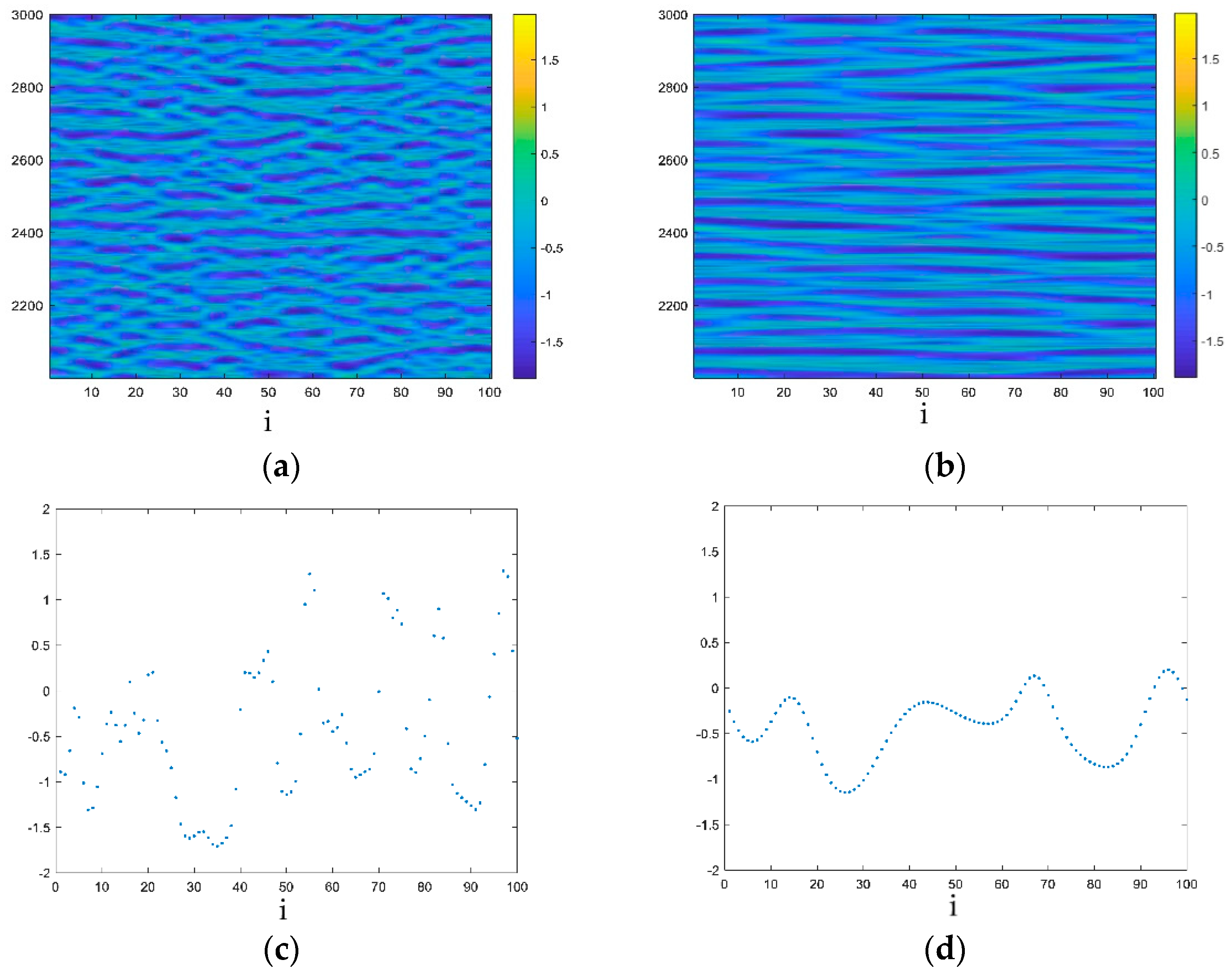
Neuronal network spatiotemporal patterns for (a) , and (b) . The corresponding snapshots for (c) , and (d) .
Figure 19.
Neuronal network spatiotemporal patterns for (a) , and (b) . The corresponding snapshots for (c) , and (d) .

Figure 20.
Phase diagram of for (a) , (b) , (c) , and (d) .

Figure 21.
Curves of for different k1.

Figure 22.
Neuronal network spatiotemporal patterns for (a) , and (b) . The corresponding snapshots at for (c) , and (d) .
Figure 22.
Neuronal network spatiotemporal patterns for (a) , and (b) . The corresponding snapshots at for (c) , and (d) .

Figure 23.
Curves of when for different q.

Figure 24.
Neuronal network spatiotemporal patterns and corresponding snapshots for different fractional-orders and coupling strengths. (a) , (b) , (c) , (d) ; (e) , (f) , (g) , (h) ; (i) , (j) , (k) , (l) .
Figure 24.
Neuronal network spatiotemporal patterns and corresponding snapshots for different fractional-orders and coupling strengths. (a) , (b) , (c) , (d) ; (e) , (f) , (g) , (h) ; (i) , (j) , (k) , (l) .

Figure 25.
for and .

Publisher’s Note: MDPI stays neutral with regard to jurisdictional claims in published maps and institutional affiliations. |
© 2021 by the authors. Licensee MDPI, Basel, Switzerland. This article is an open access article distributed under the terms and conditions of the Creative Commons Attribution (CC BY) license (https://creativecommons.org/licenses/by/4.0/).
Share and Cite
MDPI and ACS Style
Yang, X.; Zhang, G.; Li, X.; Wang, D. The Synchronization Behaviors of Coupled Fractional-Order Neuronal Networks under Electromagnetic Radiation. Symmetry 2021, 13, 2204. https://0-doi-org.brum.beds.ac.uk/10.3390/sym13112204
AMA Style
Yang X, Zhang G, Li X, Wang D. The Synchronization Behaviors of Coupled Fractional-Order Neuronal Networks under Electromagnetic Radiation. Symmetry. 2021; 13(11):2204. https://0-doi-org.brum.beds.ac.uk/10.3390/sym13112204
Chicago/Turabian StyleYang, Xin, Guangjun Zhang, Xueren Li, and Dong Wang. 2021. "The Synchronization Behaviors of Coupled Fractional-Order Neuronal Networks under Electromagnetic Radiation" Symmetry 13, no. 11: 2204. https://0-doi-org.brum.beds.ac.uk/10.3390/sym13112204
Note that from the first issue of 2016, this journal uses article numbers instead of page numbers. See further details here.