
An Uncertain APP Model with Allowed Stockout and Service Level Constraint for Vegetables

1
School of Information Engineering, Shandong Youth University of Political Science, Jinan 250103, China
2
Key Laboratory of Intelligent Information Processing Technology and Security in Universities of Shandong, Jinan 250103, China
3
Business School, Shandong Normal University, Jinan 250014, China
*
Author to whom correspondence should be addressed.
Symmetry 2021, 13(12), 2332; https://doi.org/10.3390/sym13122332
Submission received: 27 October 2021
/
Revised: 17 November 2021
/
Accepted: 22 November 2021
/
Published: 5 December 2021
(This article belongs to the Special Issue Fuzzy Set Theory and Uncertainty Theory)
Abstract
:Volatile markets and uncertain deterioration rate make it extremely difficult for manufacturers to make the quantity of saleable vegetables just meet the fluctuating demands, which will lead to inevitable out of stock or over production. Aggregate production planning (APP) is to find the optimal yield of vegetables, shortage and overstock symmetry, are not conducive to the final benefit.The essence of aggregate production planning is to deal with the symmetrical relation between shortage and overproduction. In order to reduce the adverse effects caused by shortage, we regard the service level as an important constraint to meet the customer demand and ensure the market share. So an uncertain aggregate production planning model for vegetables under condition of allowed stockout and considering service level constraint is constructed, whose objective is to find the optimal output while minimizing the expected total cost. Moreover, two methods are proposed in different cases to solve the model. A crisp equivalent form can be transformed when uncertain variables obey linear uncertain distributions and for general case, a hybrid intelligent algorithm integrating the 99-method and genetic algorithm is employed. Finally, two numerical examples are carried out to illustrate the effectiveness of the proposed model.
1. Introduction
The aim of aggregate production planning (APP) is to meet the market demand and achieve the maximum profit or minimum cost by adjusting the production and other controllable factors for all kinds of products over a finite planning horizon. The relationship between shortage and overproduction is symmetrical; shortage leads to profit maximization, and overproduction leads to cost minimization. We are trying to solve the problem of balance between shortage and overproduction. In 1955, Holt et al. [1] proposed the HMMS rule, and since then researchers have developed plenty of models to solve the APP problem, such as [2,3,4,5,6,7,8]. As the initial segment of the supply chain, the production planning problem is discussed in this paper. As a special category of perishable products, the study of the APP problem of vegetables can learn from the perishable products.
Demand and deterioration rate are two important factors in vegetables’ production process. Ghare and Schrader [9] firstly assumed a constant rate and studied the perishable inventory problems with a deterministic demand. An EOQ model for items with Weibull distribution deterioration was proposed by Covert and Philip [10] in 1973. In 2016, a production planning model considering uncertain demand using two-stage stochastic programming in a fresh vegetable supply chain context was presented by Jordi Mateo et al. [11]. Meanwhile, some scholars established lots of APP models under the fuzzy environment, such as [12,13].
For the production planning problem, whether or not to allow shortages is another factor that researchers are concerned about. Although shortages and overproduction are symmetrical, in general, the probability of occurrence is also symmetrical, but in reality, shortage occurs frequently. Moreover, in the perishable products supply chain with a high deterioration rate, the demand is often backlogged deliberately to reduce losses of deterioration. As a result, more and more research studies tend to assume that being out of stock is allowed and they usually take the sales loss and opportunity cost caused by being out of stock into consideration. In 2005, Yu et al. [14] firstly proposed an integrated VMI model considering a single deteriorating item and back ordering and concluded that it was meaningful to allow shortages, especially in the case of relatively low shortage costs. Then, in 2014, Liu et al. [15] built a decision model of a simple two-echelon perishable product supply chain that considered customer returns and the split shortage penalty mechanism after the introduction of the options contract and obtained the initial order volume and options purchasing volume of the retailer.
As for the inevitable shortage, manufacturers must try their best to improve the service level and meet customer needs in order to ensure the market share. Therefore, as an important evaluation index, the service level should be taken into account in the process of production planning. However, as for the constraints of perishable goods production and inventory, most of the literature mainly paid attention to the constraints on the stock transfer and production capacity. At present, fewer studies regard the service level as a constraint. In 2012, PaulsWorm et al. [16] studied a production planning problem for a perishable product with a fixed lifetime under a service level constraint whose objective was to develop a production planning method for a perishable product with non-stationary demand and a long deterministic production lead time. Duan et al. [17] dealt with two period inventory optimization problems for perishable items, where the demand rate depended on the service level of the previous replenishment cycle, and the results indicated that the service level was an important factor that influenced the inventory policy and the enterprise should balance the service level and profits. Then Xu and Xiao [18] established an inventory control model based on service level constraints. In 2016, Xiong [19] studied the Pareto optimal area of the perishable product order timing by means of the service level and discussed a two-echelon supply chain which was comprised of a supplier and a retailer. This research might provide the retailer with valuable guidance for its decision of order timing. Above all, it is very necessary to consider the service level as an important factor to study the supply chain of perishable products.
The APP problem not only involves large amounts of data, but might be undergone by all sorts of unpredictable disruptions in actual production. Some uncertain methods are used to handle this problem. In order to study the behavior of uncertain phenomena, uncertainty theory was founded by Liu [20] in 2007 and redefined by Liu [21] in 2010. Uncertainty theory has been developed steadily and applied widely [22,23,24,25,26]. Given the production planning problem, a multi-product aggregate production planning model based on uncertainty theory was presented by Ning et al. [27] in 2013, whose studying object was the general products. Pang and Ning [28] used uncertainty theory to study the aggregate production planning problem for vegetables from the point of manufacturers. Ning, Pang and Wang [29] established an expected profit model considering preservation technology investment under the capacity constraints. On the basis of the models and aiming at the particularities of vegetables, an uncertain APP model for vegetables under the conditions of allowed stockout and service level constraints is built in this paper.
The remainder of the paper is organized as follows. In Section 2, we describe the uncertain APP problem for vegetables. Section 3 proposes an uncertain APP model for fresh vegetables. In Section 4, a crisp equivalent form of the proposed model is obtained when the variables are linear, and a hybrid intelligent algorithm is designed in the general case. Then, we give two numerical examples to illustrate the proposed models in Section 4. Finally, some conclusions are covered in Section 6.
2. Problem Description
Now we assume that a manufacturer intends to produce N different kinds of vegetables over a finite planning horizon T, including t periods. The ripe vegetables will be stored in the inventory to wait to be bought by the distributors. In the decision-making process, the manufacturer should take account of a variety of uncertain factors, try their best to make the output keep up with the demand, and realize the target of the minimum total cost during the whole horizon T. The properties of fast updating speed and volatile markets for new products make the historical data unreliable for forecasting the future demand. Moreover, the deterioration rate and demand will also be affected by the nature of the vegetables and storage conditions as well as other factors, . All of these make the deterioration rate and demand be usually obtained on the basis of the belief degree from experienced experts instead of the historical data. Furthermore, because of the uncertain deterioration rate, unfixed deterioration time and uncertain customer arrival time, it is difficult to determine how many products will go bad and when they will go bad or be sold, which might interfere with making an accurate judgment for the inventory cost and storage space occupied by per unit vegetable. In this paper, we employ uncertain variables to denote these four factors.
On the one hand, the unfixed deterioration time and uncertain deterioration rate make the unmetamorphosed part of the vegetables that can be sold eventually become unstable. On the other hand, it is extremely difficult for the manufacturer to forecast the market demand accurately because of the properties of the fast updating speed and volatile markets for new products. Therefore, it becomes very hard to make the quantity of salable vegetables just meet the fluctuating demands and will lead inevitably to being out of stock or to overproduction. So, these two cases are both considered in this paper. Other assumptions and simplifications are stated as follows:
Firstly, the vegetables will be stored in the inventory after harvest and begin deteriorating as soon as they are entered the storage. Once sold or deteriorating, this part of the vegetables will leave the storage and no longer expand the inventory cost;
Secondly, the characteristics of freshness and deterioration make it difficult to sell the vegetables across the planning period. Hence, there is no beginning inventory in each period;
Thirdly, the total cost consists of the production cost, inventory cost, deterioration cost, shortage cost and overproduction cost;
Fourthly, the production cost, processing cost, shortage cost, overproduction cost and maximum warehouse space are deterministic and constant.
To sum up, , , , are set as uncertain variables which are independent of each other, and is set as the decision variable, . The notations of the APP problem are shown in Table 1.
3. Model Formulation
In this section, we build an uncertain programming model according to the description for vegetables’ APP problem. The objective function and the constraints are constructed as below.
3.1. Objective Function
The total cost includes the following:
Firstly, the total production cost ;
Secondly, the total inventory cost ;
Thirdly, the total deterioration cost
It is well known that for the amount of perished vegetables , we not only lose the production cost in vain, but also need pay additional processing cost ;
Fourthly, the total shortage cost , where ;
Fifthly, the total overproduction cost , where .
As a consequence, the objective function about the total cost is
3.2. Constraints
3.2.1. Service-Level Constraint
It is inevitable for vegetables to be out of stock, and in the actual production, the under-supply of a product is one of the main factors that contribute to customer service levels drop. In order to ensure the market share and meet the customer demand, we regard the service level as an important constraint and construct the following chance constraint:
where is the service level, and .
3.2.2. Inventory Capacity Constraint
The actual production will be restricted by limited resources, and inventory limitation is introduced into this APP problem. Volatile market demand, uncertain deterioration rate and other disruptions make the manufacturer cannot set an accurate storage constraints. So, the chance constraint on the uncertain measure that the storage space taken up by all products does not exceed the maximum warehouse space available is not less than in period t is as follows,
where is denoted as the confidence level, and .
3.3. Model
Different managers have different attitudes towards the risk in the decision-making process. In this paper, we assume that the decision maker wants to obtain a minimum expected cost under chance constraints, then the APP model may be built as follows,
4. Solving Method
In uncertainty theory, uncertainty distributions are usually used to depict uncertain variables. For model (4), two methods must be proposed to obtain the optimal solution because of the form of and . When the uncertain variables all obey linear uncertain distributions, a crisp form can be deduced by some theorems, while if the uncertain variables follow different kinds of uncertain distributions, a hybrid algorithm needs to be used to solve the uncertain model.
4.1. Equivalent Crisp Form
In this subsection, we assume that all uncertain variables obey linear uncertain distribution, then the equivalent crisp form can be obtained by uncertainty theory [20]. The information of these uncertain variables are shown in Table 2.
According to uncertain expectation [20], Equation (1) can be converted into
where , . For this uncertain APP problem, we are not sure whether it is out of stock or overproduction. According to reference [27], the second is the most suitable choice for this model. As a result, the objective function can be further transformed into the following form,
where .
According to reference [27], we can obtain
where .
Above all, we obtain the deterministic form of model (4),
Obviously, Equation (5) is a nonlinear programming and it can be solved by traditional optimization methods.
4.2. Genetic Algorithm Combined with 99-Method
In some cases, it will become difficult to transform the uncertain model into a crisp form. The 99 method can be employed to gain approximate values of the objective function and constraints. Genetic algorithm can be used to find the optimal solution of the model. Then, we can integrate genetic algorithm and the 99 method to solve Equation (4) for the cases.
According to reference [21], the uncertain variables has the 99 method as follow,
| 0.01 | 0.02 | |
| … | 0.99 | |
| … |
The uncertain variables have a 99 method as follow,
| 0.01 | 0.02 |
| … | 0.99 |
| … |
Then, the objective function
has a 99 table ( and k is an integer) as follow.
| … | … | |
| … | ||
| + | ||
| + | … |
Then the objective value in Equation (4) can be approximated by the following function value
For the constraints, we can convert them into deterministic form by reference [23], and Equation (2) is equivalent to
Equation (3) can be transformed into
Then we can use the genetic algorithm and direct search toolbox (GADST) in MATLAB to search for the optimal solutions for Equation (4).
5. Numerical Examples
Two numerical examples are given to illustrate the proposed model in Section 4.
Example 1 Assume that a manufacturer plans to produce two kinds of vegetables during two periods and all uncertain variables obey linear uncertain distributions. Information of the numerical instance including uncertain variables and various deterministic costs is shown in Table 3. In addition, other relevant parameters are presented as follows, , .
In accordance with the information from Table 3, the deterministic Equation (5) can be further converted into
where
This nonlinear programming model can be solved by the optimization software Lingo, and we obtain the optimal objective value , which represents the minimum total cost of this production planning problem. The optimal solutions of the output are listed in Table 4.
Example 2 Consider an APP model with two kinds of vegetables during two periods (the related data are listed in Table 5), where the uncertain variables obey different kinds of uncertain distributions. The uncertain model cannot be transformed into a crisp equivalent one. We use the genetic algorithm and direct search toolbox in MATLAB 8.5 to solve this example. The relevant parameters in the genetic algorithm are presented as follows: ’PopulationSize’ = 45, ’CrossoverFraction’ = 0.35, and ’PopInitRange’ = [0; 10]. We set ’rng(0, ’twister’)’ for reproducibility. In addition, the confidence levels are set as , and the largest inventory capacity is set as .
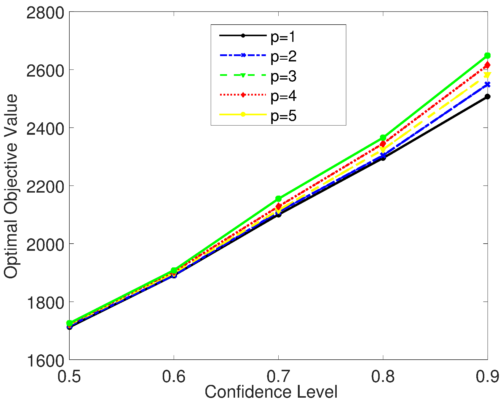
After 81 generations, we obtain that the minimum total cost is and the values of the decision variables are shown in Table 6. In order to demonstrate the relationship between the total cost and the service level for this APP problem, we assign different values to confidence level and overproduction cost p (for simplicity, we assume ) to observe the changes of the minimal cost. Their optimal objective values are shown in Table 7, and we can find the changing trend of the optimal values from Figure 1.
From these five gradual rising lines, we can find that the optimal total cost rises with the increase in service level gradually at the same overproduction cost, which implies that there is a reciprocal relationship between the total cost and service level, alerting the decision makers to handle this conflict reasonably. In addition, from the look of the whole figure, we can also find that the bigger the value of the overproduction cost, the larger the increasing range of the optimal objective value with the increase in service level. This plays a large role in revealing that a bigger overproduction cost will lead to a faster speed at which the total cost increases with the service level, especially the higher service level. Hence, the manufacturer should reasonably control the quantity and cost of overproduction.
The feasibility of the model is verified by numerical examples. The experimental results of the numerical examples provide a theoretical basis and reference for APP decision makers in the actual environment.
6. Conclusions
This paper proposed an APP model for vegetables under the condition of allowed stockout and considering the service level constraint from the point of the manufacturer in an uncertain environment. In accordance with the characteristics of the APP problem for vegetables, the deterioration rate, market demand and other factors are described by uncertain variables. Then, a crisp equivalent form is given when these uncertain variables obey linear uncertain distributions, while a hybrid intelligent algorithm integrating the 99 method and genetic algorithm is employed to solve the uncertain model for the general case. Finally, two numerical examples are given to illustrate the proposed models, and we conclude that the manufacturer should deal with the reciprocal relationship between total cost and service level reasonably.
We will continue to study the problem of model construction considering various factors such as being out of stock, service level and vegetable freshness. We will also study modeling and solving problems with some parameters as uncertain random variables.
Uncertain random variables, proposed by Liu [30] in 2013, are used to model complex systems that contain both uncertainty and randomness. In this paper, we only discussed the case of uncertainty in APP; we will study the construction of an uncertain random APP model in the future.
Author Contributions
Conceptualization, Y.N.; methodology, N.P.; validation, X.C.; data curation, S.W.; writing—original draft preparation, Y.N.; writing—review and editing, Y.N. and S.W. All authors have read and agreed to the published version of the manuscript.
Funding
This research was funded by the Natural Science Foundation of Shandong Province grant number ZR2014GL002.
Institutional Review Board Statement
Not applicable.
Informed Consent Statement
Not applicable.
Data Availability Statement
Not applicable.
Conflicts of Interest
The authors declare no conflict of interest.
References
- Holt, C.; Modigliani, F.; Simon, H. A linear decision rule for production and employment scheduling. Manag. Sci. 1955, 2, 1–30. [Google Scholar] [CrossRef]
- Saad, G. An overview of production planning model: Structure classification and empirical assessment. Int. J. Prod. Res. 1982, 20, 105–114. [Google Scholar] [CrossRef]
- Akinc, U.; Roodman, G.M. A new approach to aggregate production planning. IIE Trans. 1982, 18, 84–94. [Google Scholar] [CrossRef]
- Jamalnia, A.; Yang, J.; Xu, D.; Feili, A. Novel decision model based on mixed chase and level strategy for aggregate production planning under uncertainty: Case study in beverage industry. Comput. Ind. Eng. 2017, 114, 54–68. [Google Scholar] [CrossRef] [Green Version]
- Mehdizadeh, E.; Niaki, S.; Hemati, M. A bi-objective aggregate production planning problem with learning effect and machine deterioration: Modeling and solution. Comput. Oper. Res. 2018, 91, 21–36. [Google Scholar] [CrossRef]
- Rasmi, S.; Kazan, C.; Türkay, M. A multi-criteria decision analysis to include environmental, social, and cultural issues in the sustainable aggregate production plans. Comput. Ind. Eng. 2019, 132, 348–360. [Google Scholar] [CrossRef]
- Jang, J.; Chung, B. Aggregate production planning considering implementation error: A robust optimization approach using bi-level particle swarm optimization. Comput. Ind. Eng. 2020, 142, 106367. [Google Scholar] [CrossRef]
- Rahmani, D.; Zandi, A.; Behdad, S.; Entezaminia, A. A light robust model for aggregate production planning with consideration of environmental impacts of machines. Oper. Res. 2021, 21, 273–297. [Google Scholar] [CrossRef]
- Ghare, P.M.; Schrader, S.F. A model for exponentially decaying inventory. J. Ind. Eng. 1963, 14, 238–243. [Google Scholar]
- Covert, R.P.; Philip, G.C. An EOQ model for items with weibull distribution deterioration. AIIE Trans. 1973, 5, 323–326. [Google Scholar] [CrossRef]
- Jordi, M.; Pla, L.M.; Francesc, S.; Adela, P. A production planning model considering uncertain demand using two-stage stochastic programming in a fresh vegetable supply chain context. Springerplus 2016, 5, 1–16. [Google Scholar]
- Mula, J.; Poler, R.; Garcia-Sabater, J.P.; Lario, F.C. Models for production planning under uncertainty: A review. Int. J. Prod. Econ. 2006, 103, 271–285. [Google Scholar] [CrossRef] [Green Version]
- Wang, R.; Fang, H. Aggregate production planning with multiple objectives in a fuzzy environment. Eur. J. Oper. Res. 2001, 133, 521–536. [Google Scholar] [CrossRef]
- Yu, Y.G.; Xiong, Y.; Dong, Y.; Huang, G.Q. An integrated vendor-managed-inventory model for deteriorating item allowing shortage. Oper. Res. Manag. Sci. 2005, 14, 31–36. [Google Scholar]
- Liu, Y.; Pan, J.; Jin, M. Optimization strategy of perishable product supply chains considering customer returns under split shortage penalty mechanism. Logist. Technol. 2014, 33, 295–301. [Google Scholar]
- PaulsWorm, G.J.K.; Haijema, R.; Hendrix, E.M.T.; Rossi, R.; Vorst, J. Production planning of a perishable product with lead time and non-stationary demand. In Proceedings of the 17th International Symposium on Inventories, Budapest, Hungary, 20–24 August 2012; Volume 5, pp. 20–24. [Google Scholar]
- Duan, Y.R.; Fu, Q.C.; Li, G.P. Optimal inventory policy for perishable items with service-level-dependent demand rate. Oper. Res. Manag. Sci. 2015, 24, 65–75. [Google Scholar]
- Xu, D.G.; Xiao, R.B. Research on inventory policy of grain and oil under restriction of service level. Appl. Res. Comput. 2011, 28, 1389–1391. [Google Scholar]
- Xiong, H.Q. An analysis of perishable product order timing in perspective of service level. Ind. Eng. J. 2016, 19, 24–29. [Google Scholar]
- Liu, B. Uncertainty Theory, 2nd ed.; Springer: Berlin/Heidelberg, Germany, 2007; pp. 10–84. [Google Scholar]
- Liu, B. Uncertainty Theory: A Branch of Mathematics for Modeling Human Uncertainty; Springer: Berlin/Heidelberg, Germany, 2010. [Google Scholar]
- Liu, B. Theory and Practice of Uncertain Programming, 2nd ed.; Springer: Berlin/Heidelberg, Germany, 2009; pp. 2–56. [Google Scholar]
- Liu, B. Uncertain risk analysis and uncertain reliability analysis. J. Uncertain Syst. 2010, 4, 163–170. [Google Scholar]
- Liu, J.; Ning, Y.; Yu, X. Reverse logistics network in uncertain environment. Inf. Int. Interdiscip. J. 2013, 16, 1243–1248. [Google Scholar]
- Ning, Y.; Yan, L.; Xie, Y. Mean-TVaR model for portfolio selection with uncertain returns. Inf. Int. Interdiscip. J. 2013, 16, 977–985. [Google Scholar]
- Yu, X. A stock model with jumps for uncertain markets. Int. J. Uncertain Fuzziness Knowl.-Based Syst. 2012, 20, 421–432. [Google Scholar] [CrossRef]
- Ning, Y.; Liu, J.; Yan, L. Uncertain aggregate production planning. Soft Comput. 2013, 17, 617–624. [Google Scholar] [CrossRef]
- Pang, N.; Ning, Y. An Uncertain Aggregate Production Planning Model for Vegetables. In Proceedings of the 2017 13th International Conference on Natural Computation, Fuzzy Systems and Knowledge Discovery (ICNC-FSKD 2017), Guilin, China, 29–31 July 2017; pp. 1351–1360. [Google Scholar]
- Ning, Y.; Pang, N.; Wang, X. An Uncertain aggregate production planning model considering investment in vegetable preservation technology. Math. Probl. Eng. 2019, 2019, 8505868. [Google Scholar] [CrossRef] [Green Version]
- Liu, Y. Uncertain random variables: A mixture of uncertainty and randomness. Soft Comput. 2013, 4, 625–634. [Google Scholar] [CrossRef]
Figure 1.
The changing trend of optimal objective value.


Table 1.
Notations of the APP problem.
| Notation | Meaning |
|---|---|
| N | Types of vegetables |
| T | Planning horizon |
| f | Total cost function over T |
| Demand for the nth vegetable in period t (units) | |
| Deterioration rate of the nth vegetable in period t, | |
| Unit processing cost for the nth vegetable in period t ($/unit) | |
| Unit production cost of the nth vegetable in period t ($/unit) | |
| Total production of the nth vegetable in period t (units) | |
| Unit inventory cost of the nth vegetable in period t ($/unit) | |
| Unit shortage cost of the nth vegetable in period t ($/unit) | |
| Quantities of shortage of the nth vegetable in period t (units) | |
| Unit overproduction cost of the nth vegetable in period t ($/unit) | |
| Quantities of overproduction of the nth vegetable in period t (units) | |
| Warehouse space per unit of the nth vegetable in period t (/unit) | |
| Maximum warehouse space available in period t () |
Table 2.
Uncertain linear distributions.
| Uncertain Variable | Linear Uncertain Distribution |
|---|---|
Table 3.
Information of Example 1.
| Item | Period 1 | Period 2 |
|---|---|---|
| 4 | 6 | |
| 5 | 8 | |
| 2 | 1 | |
| 2 | 3 | |
| 2 | 1 | |
| 1 | 2 | |
| 1 | 1 | |
| 2 | 1 |
Table 4.
Optimal output of the production planning in Example 1.
| Item | Period 1 | Period 2 |
|---|---|---|
| 76.7008 | 67.9473 | |
| 77.7044 | 103.7260 |
Table 5.
Information of Example 2.
| Item | Period 1 | Period 2 |
|---|---|---|
| 4 | 6 | |
| 5 | 8 | |
| 2 | 1 | |
| 2 | 3 | |
| 2 | 2 | |
| 2 | 2 | |
| 3 | 3 | |
| 3 | 3 |
Table 6.
Optimal output of the production planning in Example 2.
| Item | Period 1 | Period 2 |
|---|---|---|
| 113.9636 | 115.6818 | |
| 100.6382 | 118.7673 |
Table 7.
The changes of optimal values under different service levels and overproduction costs.
| = 0.5 | = 0.8 | ||||
|---|---|---|---|---|---|
| 2295.24 | 2506.74 | ||||
| 2304.33 | 2549.23 | ||||
| 2324.86 | 2582.49 | ||||
| 2345.19 | 2615.75 | ||||
| 2365.44 | 2649.01 |
Publisher’s Note: MDPI stays neutral with regard to jurisdictional claims in published maps and institutional affiliations. |
© 2021 by the authors. Licensee MDPI, Basel, Switzerland. This article is an open access article distributed under the terms and conditions of the Creative Commons Attribution (CC BY) license (https://creativecommons.org/licenses/by/4.0/).
Share and Cite
MDPI and ACS Style
Ning, Y.; Pang, N.; Wang, S.; Chen, X. An Uncertain APP Model with Allowed Stockout and Service Level Constraint for Vegetables. Symmetry 2021, 13, 2332. https://0-doi-org.brum.beds.ac.uk/10.3390/sym13122332
AMA Style
Ning Y, Pang N, Wang S, Chen X. An Uncertain APP Model with Allowed Stockout and Service Level Constraint for Vegetables. Symmetry. 2021; 13(12):2332. https://0-doi-org.brum.beds.ac.uk/10.3390/sym13122332
Chicago/Turabian StyleNing, Yufu, Na Pang, Shuai Wang, and Xiumei Chen. 2021. "An Uncertain APP Model with Allowed Stockout and Service Level Constraint for Vegetables" Symmetry 13, no. 12: 2332. https://0-doi-org.brum.beds.ac.uk/10.3390/sym13122332
Note that from the first issue of 2016, this journal uses article numbers instead of page numbers. See further details here.