Calculating Beamforming Vectors for 5G System Applications

Abstract

The growing demand for broadband Internet services is forcing scientists around the world to seek and develop new telecommunication technologies. With the transition from the fourth generation to the fifth generation wireless communication systems, one of these technologies is beamforming. The need for this technology was caused by the use of millimeter waves in data transmission. This frequency range is characterized by heavy path loss. The beamforming technology could compensate for this significant drawback. This paper discusses basic beamforming schemes and proposes a model implemented on the basis of QuaDRiGa. The model implements a MIMO channel using symmetrical antenna arrays. In addition, the methods for calculating the antenna weight coefficients based on the channel matrix are compared. The first well-known method is based on the addition of cluster responses to calculate the coefficients. The proposed one uses the singular value decomposition of the channel matrix into clusters to take into account the most correlated information between all clusters when calculating the antenna coefficients. According to the research results, the proposed method for calculating the antenna coefficients allows an increase in the SNR/SINR level by 8–10 dB on the receiving side in the case of analog beamforming with a known channel matrix.

1. Introduction

Symmetry is an international peer-reviewed journal, one of the areas of which is devoted to the study of information technology and electronics. This direction addresses the problems of telecommunications and next-generation communication systems. In this article, we raise the issue of beamforming technology, which is an integral part of fifth generation systems. A ubiquitous change from 4G (fourth generation) to 5G (fifth generation) in wireless communication systems is on the way in the nearest future. Nowadays, there are many examples of successful implementation of 5G networks in the USA, Germany, South Korea and other countries [1]. Behind a simple change in the name lie big changes in the wireless telecommunications industry and the years of scientific and engineering work. These changes affected all the qualitative and quantitative features of the new systems. The introduction of the 5G technologies affects many aspects of our lives. First, the data transfer speed significantly increases because of the higher bandwidth. This expands the possibilities of VR video streaming (virtual reality) and remote services to use programs. Next, the delay in data transmission is reduced. This allows real-time control of remote devices over the Internet. Finally, it is possible to connect more devices to the Internet. This takes a step towards the ideas of “Smart Home”, “Smart Manufacturing” and others. These advantages are due to the move towards the millimeter frequency range. However, there is one problem with this move. This is a significant signal attenuation when the distance and frequency increase. Without compensating for this disadvantage, most of 5G benefits would be unrealizable. Ultimately, this would lead to a reduction in the cell radius or to an increase in the power consumption for signal transmission. The beamforming technology has been proposed as a solution that allows the power to be focused in the direction of the receiver. This technology is now finding its practical application after multi-array antennas have rapidly been implemented. The research into beamforming technology is of great importance today. Most of these studies are carried out by means of simulation, which allows expanding the number of researchers and reducing the costs inherent to natural experiment. As part of the 5G studies, a great number of statistical models have already been developed. The examples of such developments include the ns-3 network simulator [2] and the QuaDRiGa universal channel model supporting a millimeter-wave range [3,4,5]. In continuation of these works, we implemented a model in MATLAB software based on QuaDRiGa that provides the estimation of the signal power at the receiving part equipped with the beamforming technology. This paper describes the model and presents the simulation results for stationary scenarios of signal propagation in an urban environment using millimeter-wave frequencies. In addition, we propose a method for calculating the antenna weight coefficients and compare it with the existing method used in the ns-3.

The essence of the beamforming technology is that an interference effect occurs between the signals sent from different antennas. This interference increases the signal amplitude at the receiver side. In other directions, the amplitude decreases. The beamforming schemes are subdivided into analog, digital and hybrid [6].

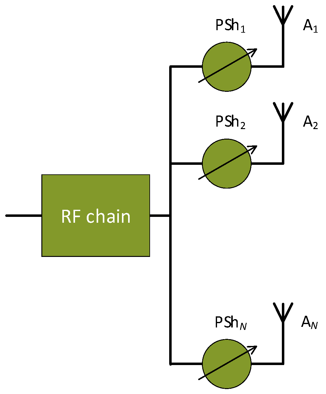
The basic idea of analog beamforming is to control the phase of each transmitted signal using inexpensive phase shifters. Analog beamforming affects the gain of the antenna array, thus improving its coverage. Only one beam can be generated per set of antenna elements, in contrast to a digital beamforming scheme. The antenna gain caused by analog beamforming partially compensates for the high millimeter-wave path loss. Therefore, analog beamforming is a must for 5G millimeter-wave frequencies. Figure 1 shows a block diagram of the analog scheme of beamforming [6].

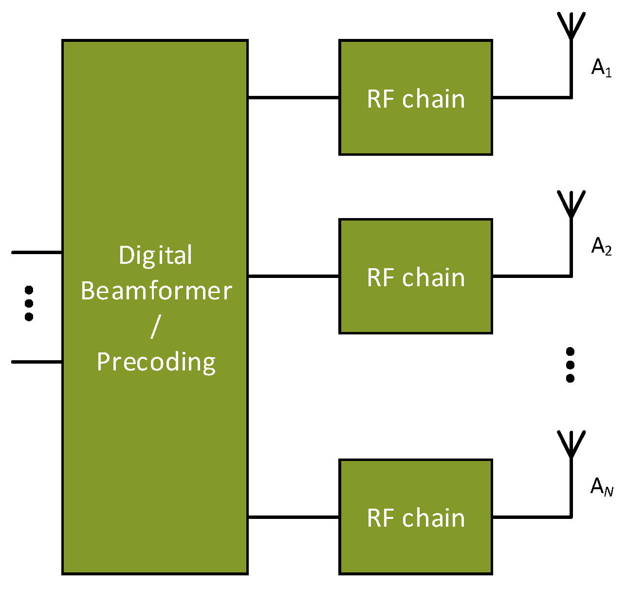
In digital beamforming, the signal is pre-encoded before being sent to the analog RF (radio frequency) circuit. Several beams (one for each user) can be generated simultaneously from the same set of antenna elements. A base station needs multiple RF circuits, one for each user. Digital beamforming increases cell throughput because the same physical resource block (PRB) can be used to transmit data for multiple users at the same time. Figure 2 shows a block diagram of the digital beamforming scheme.

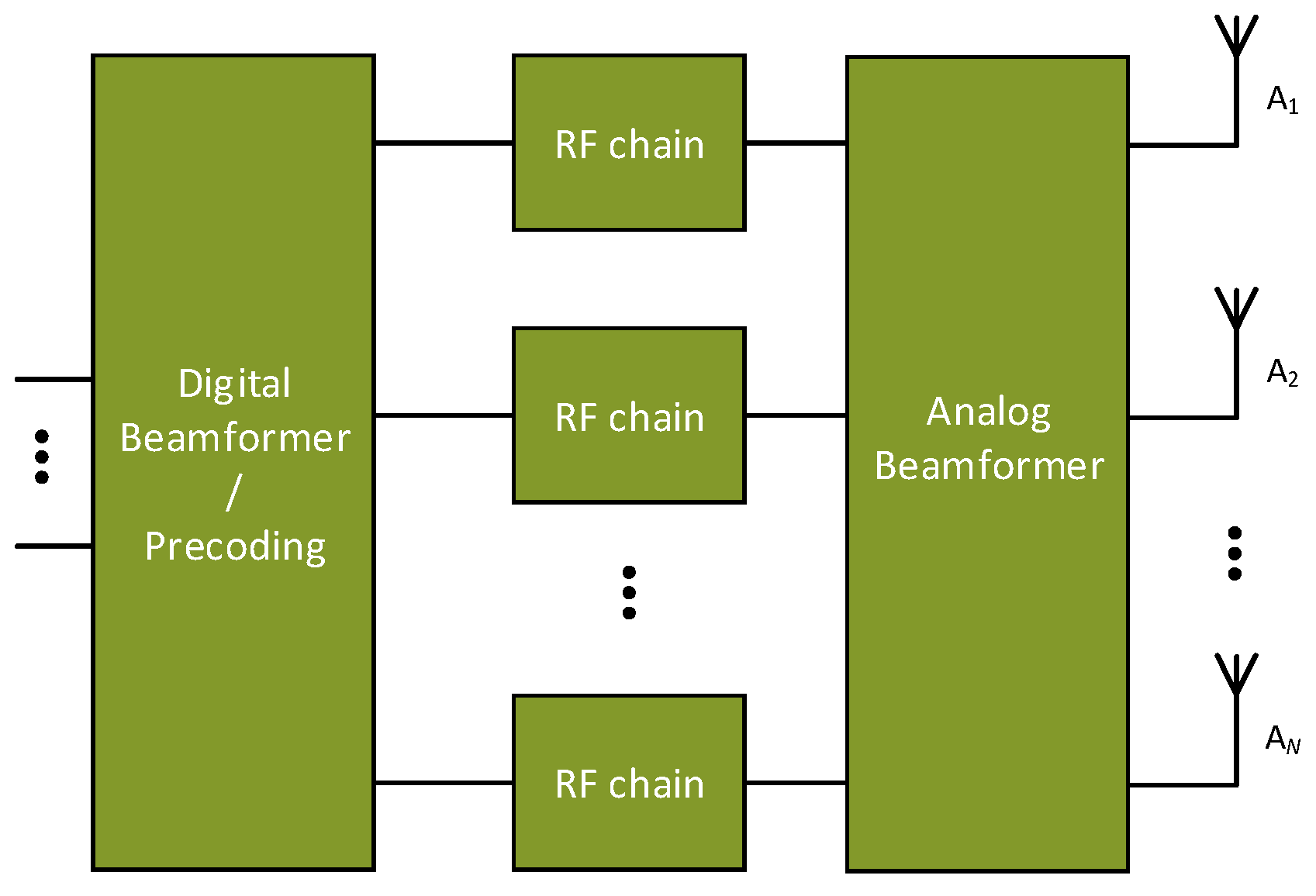
Hybrid beamforming is a combination of analog and digital beamforming. It has the advantages of both methods. This method requires fewer RF chain (radio frequency) than digital beamforming. It is also more flexible than analog beamforming. Therefore, it is assumed that 5G base stations will use some realization of hybrid beamforming [7]. The block diagram of the hybrid beamforming scheme is shown in Figure 3 [6].

Regardless of the beamforming scheme, each of them assumes the awareness of the current state of the channel between a BS and a user terminal (UT). In the best case, the channel state matrix $\mathbf{H}$ is known. Based on this matrix, antenna weights for analog beamforming or precoding matrix for digital beamforming are calculated. The article presents one of the well-known methods for calculating weight coefficients and the one proposed by the authors. In addition, the paper [8] should be mentioned, which addresses the same area of research. In this paper, authors propose a zero-forcing based coordinated beamforming scheme and consider wireless transmissions over directional multiple-input single-output (MISO) two wave with diffuse power (TWDP) fading channels. Another good work on this topic is [9]. In this paper, the authors propose a joint Tx–Rx beamforming with beam selection and combining technique. This beamforming scheme improves the performance of a wireless communications system using electronically steerable antenna arrays.

2. Materials and Methods for Calculating Antenna Weight Coefficients

The matrix of channel coefficients $H$ has the dimensions $U$ × $S$ × $N$, where $U$ is the number of receiving elements of the antenna array, $S$ is the number of transmitting antenna elements and $N$ is the number of clusters. A cluster is a group of beams reflected from one object in free space. All these beams, reflected from the object, are characterized by small delays relative to each other and strong correlation properties. Such cluster structure is explained by the fact that real objects are not points in space, but rather volumetric objects of a certain shape and, in most cases, with an uneven reflecting surface. Therefore, this model describes a more realistic environment, which allows for reliable simulation data. The number of clusters and their properties depend on the selected scenario. For example, according to the recommendations of 3GPP_TR38.901 [10], for a macro urban environment with no line-of-sight (NLOS), there are 20 beams, while in a scenario describing a rural area, there are only 10 beams. In the channel matrix, the clusters are arranged in order of increasing latency. The $U$ × $S$ × 1 section corresponds to a direct beam for LOS and the first reflected beam for NLOS. Each value located at the intersection of $u$, $s$ and $n$ is a complex value that characterizes the changes in the amplitude and phase of the signal during transmission from the $u$ transmitting element to the $s$ receiving element for the $n$ cluster. In the general case, the vector along the $N$ axis can be considered as the pulse response of a pair of two antenna array elements.

The beamforming technology is based on maximizing the following equation:

$$G=\arg \max \left\{{\displaystyle \sum _{n=1}^N{\left|{w^{\prime }}_{\mathrm{rx}}\times H_n\times w_{\mathrm{tx}}\right|}^2}\right\},$$

(1)

where $H_n$ is a matrix of dimension $U$ × $S$ corresponding to the cluster $n$, $w_{\mathrm{rx}}$ is a column vector of antenna coefficients of dimension $U\times 1$, $w_{\mathrm{tx}}$ is a column vector of antenna coefficients of dimension $S\times 1$, $G$ is a beamforming gain and sign «${}^{\prime }$» means Hermitian conjugation.

Thus, you should find such $w_{\mathrm{rx}}$ and $w_{\mathrm{tx}}$ values that will allow you to get the maximum value of $G$.

Next, we will consider several methods for calculating the beamforming vectors at the receiving and transmitting sides.

Method 1. The first method to be mentioned for calculating the beamforming vectors is described in [2,11]. This method is used in the ns-3 simulator, and the calculation requires complete information about the condition of the channel. At the transmitting and receiving sides, the matrix of channel coefficients must be known. It contains pulse responses for each pair of antenna elements at the transmitting and receiving sides.

The calculation is based on the criterion for the maximum total signal power. The following is the calculation algorithm. The first step is the calculation of the total channel matrix for all clusters according to Equation (2):

$$\widehat{H}={\displaystyle \sum _{n=1}^N{H}_n},$$

(2)

Next, the correlation matrices $Q_{\mathrm{tx}}$ and $Q_{\mathrm{rx}}$ are calculated. Matrix $Q_{\mathrm{tx}}$ determines the correlation between signal responses across all transmitting antennas (between rows of matrix $Q_{\mathrm{tx}}$). Accordingly, $Q_{\mathrm{rx}}$ determines the correlation dependence between the responses for all receiving antennas (between columns of matrix $Q_{\mathrm{rx}}$). The diagonal elements of correlation matrix are correlation coefficients. One of the properties of correlation matrices is symmetry with respect to the diagonal [12]. Equations for calculation $Q_{\mathrm{tx}}$ and $Q_{\mathrm{rx}}$ are presented below:

$$Q_{\mathrm{tx}}=\mathrm{E}\left\{H^{\prime }H\right\},$$

(3)

$$Q_{\mathrm{rx}}=\mathrm{E}\left\{H{H}^{\prime }\right\},$$

(4)

where $\mathrm{E}\left\{\right\}$ is the calculation of the expected value.

Antenna coefficient vectors are defined as eigenvectors of correlation matrices:

$$w_{\mathrm{tx}}=\mathrm{eig}\left\{Q_{\mathrm{tx}}\right\},$$

(5)

$$w_{\mathrm{rx}}=\mathrm{eig}\left\{Q_{\mathrm{rx}}\right\},$$

(6)

where $\mathrm{eig}\left\{\right\}$ is the function of calculating eigenvectors.

For the calculated values of $w_{\mathrm{rx}}$ and $w_{\mathrm{tx}}$, the following normalization equation must be executed:

$$\mathrm{tr}\left\{w_{\mathrm{tx}}{w^{\prime }}_{\mathrm{tx}}\right\}=1,$$

(7)

$$\mathrm{tr}\left\{w_{\mathrm{rx}}{w^{\prime }}_{\mathrm{rx}}\right\}=1,$$

(8)

where $\mathrm{tr}\left\{\right\}$ is the trace of a square matrix.

The obtained antenna weights are used when generating a signal at the transmitting side and when processing a signal at the receiving side. This calculation method should only be used in the case of analog beamforming. There is no way to distribute the beam among the clusters so one beam is calculated for all clusters. This beam will allow you to get the most power at the receiving side.

Method 2. As in the previous method, vectors of antenna coefficients $w_{\mathrm{rx}}$ and ${\mathbf{w}}_{\mathrm{tx}}$ are calculated on the basis of a two-dimensional matrix $\widehat{H}$. The more general information about all clusters is contained in the final matrix of channel coefficients, the greater signal amplification will be observed at the receiving side. The proposed calculation method differs from the previous one in that it has the operation for obtaining a common two-dimensional channel matrix $\widehat{H}$ for clusters.

Initially, a three-dimensional channel matrix is initially converted into a two-dimensional one as follows:

$$H\to \tilde{H}=\mathrm{conc}\left\{\mathrm{vec}(H_1),\mathrm{vec}(H_2),\dots ,\mathrm{vec}(H_N)\right\},$$

(9)

where $\mathrm{vec}(\dots )$ is the function of transforming a matrix of dimension $U\times S$ into a column vector $US\times 1$ and $\mathrm{conc}\left\{\right\}$ is the function of concatenating arrays of the same dimensions.

Matrix $H$ has dimension $US\times N$.

Next, a singular value decomposition of the resulting two-dimensional matrix is performed:

$$H=\mathrm{svd}\left\{H\right\}=D\cdot A\cdot V^{\prime },$$

(10)

where $\mathrm{svd}\left\{\right\}$ is the singular value decomposition operation, $D$ is the left-singular vectors of $H$, $V$ is the right-singular vectors of $H$.

The final matrix is formed by transforming the first singular vector of matrix $D$:

$$\tilde{h}={\tilde{D}}_{l,1},l=1,2,\dots ,L,$$

(11)

$$h\to \widehat{H}={({\widehat{h}}_{u,s})}_{u=1,s=1}^{U,S},$$

(12)

where $L$ is the value equal to the product of the number of receiving antennas $U$ by the number of transmitting antennas $S$.

Further calculation of the beamforming vectors can repeat the calculation algorithm described in Formulas (3)–(6). Moreover, the resulting beamforming vectors of antenna can be considered as left and right vectors of the singular value decomposition of matrix $\widehat{H}$:

$$\widehat{H}=\mathrm{svd}(\widehat{H})=\widehat{D}\cdot \widehat{A}\cdot \widehat{V^{\prime }},$$

(13)

$$w_{\mathrm{tx}}={V^{\prime }}_{s,1},s=1,2,\dots ,S,$$

(14)

$$w_{\mathrm{rx}}=D_{u,1},u=1,2,\dots ,U.$$

(15)

The beamforming vectors must also satisfy the normalization Equations (7) and (8).

The presented methods for the optimal calculation of beamforming vectors are of theoretically directed interest and find their application in simulating beamforming algorithms. These algorithms show the maximum possible power that can be achieved if there is absolute knowledge of the transmission channel matrix. In practice, it is impossible to obtain such comprehensive information about the channel, especially when using large multi-element antenna arrays. In real systems, the channel knowledge is partial. Some of these algorithms are described in [13].

3. Results and Simulation

QuaDRiGa (Quasi Deterministic Radio Channel Generator) is a model designed to simulate MIMO radio channels under various configurations and radio propagation conditions. This model is based on well-known geometric models of wireless channels such as SCM and WINNER. It also employs new approaches to simulation by utilizing additional functions. These functions allow simulating dynamic scenarios including both the movement of user terminals (UT) and the joint movement of BS and UT. In our model, QuaDRiGa was used to obtain realistic channel matrices under various scenarios, propagation conditions and various MIMO antenna configurations. More details about all the capabilities of QuaDRiGa can be found in [5].

The authors in [5] describe the QuaDRiGa approach as a “statistical ray-tracing model”. The main feature of this approach is that clusters are used to calculate the channel matrix. The clusters are distributed randomly. This is the essence of “statistical” for this model. The model does not need an exact geometric representation of the propagation environment. The path in the model is determined by the angle of departure (AoD), the angle of arrival (AoA) and path length. For QuaDRiGa model, the authors in [5] indicate the following:

• Quadriga uses 8–20 clusters to simulate a typical propagation environment for scenarios with carrier frequencies up to 6 GHz.
• Each cluster consists of 20 sub-paths. The total number of sub-paths ranges from 160 to 400. Each sub-path is modeled as a single reflection.
• The sum of 20 sub-paths in one cluster is one resulting path.
• Each path is represented as channel coefficients between each pair of MIMO system antenna elements.

3.1. Simulation

One of the main parameters characterizing a data transmission channel is signal-to-noise ratio (SNR) at the receiving side. The SNR value in communication systems affects many qualitative characteristics: the data transfer rate, the bit error rate (BER) and packet error rate (PER). An increase in PER and BER can lead to increased network layer delay because of repeated packets. The beamforming technology, in general, provides the increase of the energy efficiency of data transmission systems by means of a more rational distribution of the radiated power. This energy efficiency gain can be used to both increase base station coverage and reduce transmitter power consumption. The required SNR level in the case of beamforming will be provided over longer distances than in systems without beamforming. Increasing the BS coverage will reduce their number, which in turn will affect the cost of network organization. Another method is to reduce the power consumption of beamforming systems while maintaining the required BS coverage and reducing the cost of equipment. Therefore, the SNR at the receiver side can be used to determine the efficiency of the beamforming technology.

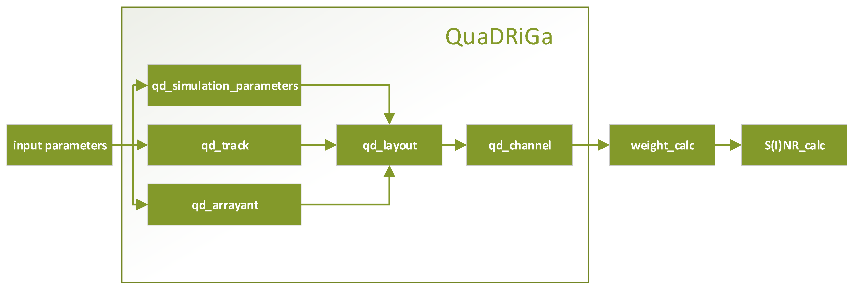
To calculate the SNR level of the user equipment that employs the beamforming technology, we developed the model in the MATLAB software. The block diagram of the model is shown in Figure 4.

This model allows you to calculate the SNR level for any network configuration and different scenarios, including propagation of radio signal in an urban environment, rural areas, free space or in a building.

QuaDRiGa is implemented in MATLAB/Octave. The model was created using an object-oriented framework that includes classes, methods and functions. The model has a convenient user interface. Class parameters can be manipulated by the user [5].

The main QuaDRiGa classes used in our model are (Figure 4):

• “qd_simulation_parameters” defines the basic parameters and settings of the model, for example: center frequency and sample rate. It also enables and disables some of the model’s functions, such as the presence of geometric polarization, spherical waves, displaying a progress bar;
• “qd_arrayant” defines” all the functions needed to describe multi-element antenna arrays;
• “qd_track” is used to describe the user’s trajectory, speed change and radio wave propagation scenario;
• “qd_layout” combines user track and antenna properties into a common object;
• “qd_channel” is the last executable class. Objects of this class contain the final channel coefficients for each described segment of the track. It can output a matrix of channel coefficients in both the time domain and the frequency domain.

The blocks “weight_calc” and “S(I)NR_calc” were implemented by us. The “weight_calc” calculates antenna weights according to one of the methods described. The “S(I)NR_calc” calculates the SNR or SINR (signal interference noise ratio) value depending on the set scenario.

3.1.1. Input Parameters

The input parameters of the model (

Table 1. Input Parameters.

Parameter	Description
Scenario	This parameter specifies the conditions for signal propagation in the wireless channel, for example: presence or absence of line-of-sight (LOS), urban or rural area, etc.
$\mathrm{Number} \mathrm{of} \mathrm{BSs}, N_{\mathrm{BS}}$	The maximum configurable number of base stations is limited only by the required memory. The minimum is one BS.
$\mathrm{Number} \mathrm{of} \mathrm{UTs}, N_{\mathrm{UT}}$	The maximum number of UTs is not limited by the program. The minimum is one UT.
BS Position	$\mathrm{An} \mathrm{array} \mathrm{with} \mathrm{a} \mathrm{dimension} \mathrm{of} 3 \times N_{BS}$. Columns are coordinates of the BS position in the Cartesian coordinate system (x, y, z).
UT Position	$\mathrm{An} \mathrm{array} \mathrm{with} \mathrm{a} \mathrm{dimension} \mathrm{of} 3 \times N_{UT}$. Columns are coordinates of the UT position in the Cartesian coordinate system (x, y, z).
$\mathrm{Minimum} \mathrm{cell} \mathrm{radius}, R_{\min }$	This parameter limits the minimum distance from the BS to the UT.
$\mathrm{Maximum} \mathrm{cell} \mathrm{radius}, R_{\max }$	This parameter limits the maximum distance from the BS to the UT.
User Position Generation Mode	$\mathrm{The} \mathrm{program} \mathrm{supports} \mathrm{two} \mathrm{modes} \mathrm{of} \mathrm{generating} \mathrm{the} \mathrm{user} \mathrm{terminal} \mathrm{position}. \mathrm{The} \mathrm{first} \mathrm{is} \mathrm{the} \mathrm{assignment} \mathrm{of} \mathrm{coordinates} \mathrm{randomly} \mathrm{in} \mathrm{the} R_{\min }$ < r < Rmax area. The second is the manual mode.
$\mathrm{Center} \mathrm{frequency}, f_0$	Center frequency in Hz.
$\mathrm{Transmission} \mathrm{power}, P_{\mathrm{TX}}$	Transmitted signal power of the BS in dBm.
$\mathrm{Internal} \mathrm{Noise} \mathrm{Power}, N_0$	Internal noise power of the UT in dBm

) are largely determined by the capabilities of the QuaDRiGa model. The features of this model were discussed in [3,4,5]. In the implementation of our model, not all of its capabilities were used. The current version enables the implementation of only stationary scenarios that do not consider the UT movements or changes in channel conditions. Simulation of dynamic scenarios, which are much more interesting, is planned to be added in future versions of the program.

3.1.2. Scenarios of the Signal Propagation Environment

The universal model of the QuaDRiGa channel has more than a hundred scenarios that describe various conditions for radio signal propagation. Each of the scenarios characterizes the space and environment between the BS and the UT at a given time point or a given area of space, depending on whether the model is stationary or dynamic. So far, only stationary scenarios have been modeled. In general, many factors influence the conditions for radio signal propagation. They include the housing density, the height of buildings, the material of surrounding objects and the width and length of streets. Obviously, it is very difficult to quantify such parameters. Therefore, each scenario in the QuaDRiGa is characterized by a set of statistical characteristics of the signal in a particular environment. Many of these characteristics were obtained empirically. These include the number of clusters, the density of the signal cluster delay distribution, the correlation properties between clusters and between the beams of the clusters, and the calculation of the attenuation coefficient.

The scenario of radio signal propagation significantly affects the efficiency of beamforming under various conditions. A particular impact will be exerted by the presence or absence of line-of-sight (LOS or NLOS).

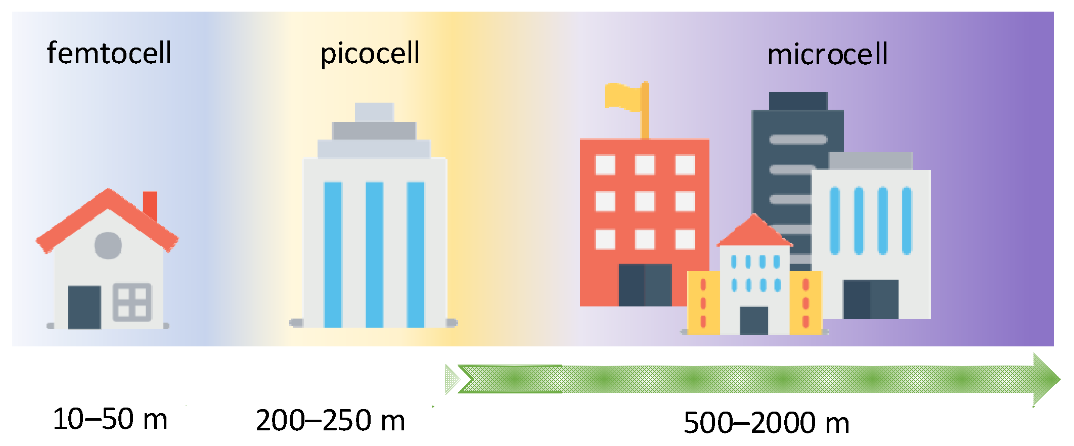
To verify the developed model and to compare the proposed algorithm for calculating antenna coefficient vectors with the existing one, several elementary cases were considered under various conditions and with different service-area: up to 50 m (femtocell), up to 250 m (picocell) and up to 2000 m (microcell). Figure 5 shows the cases considered.

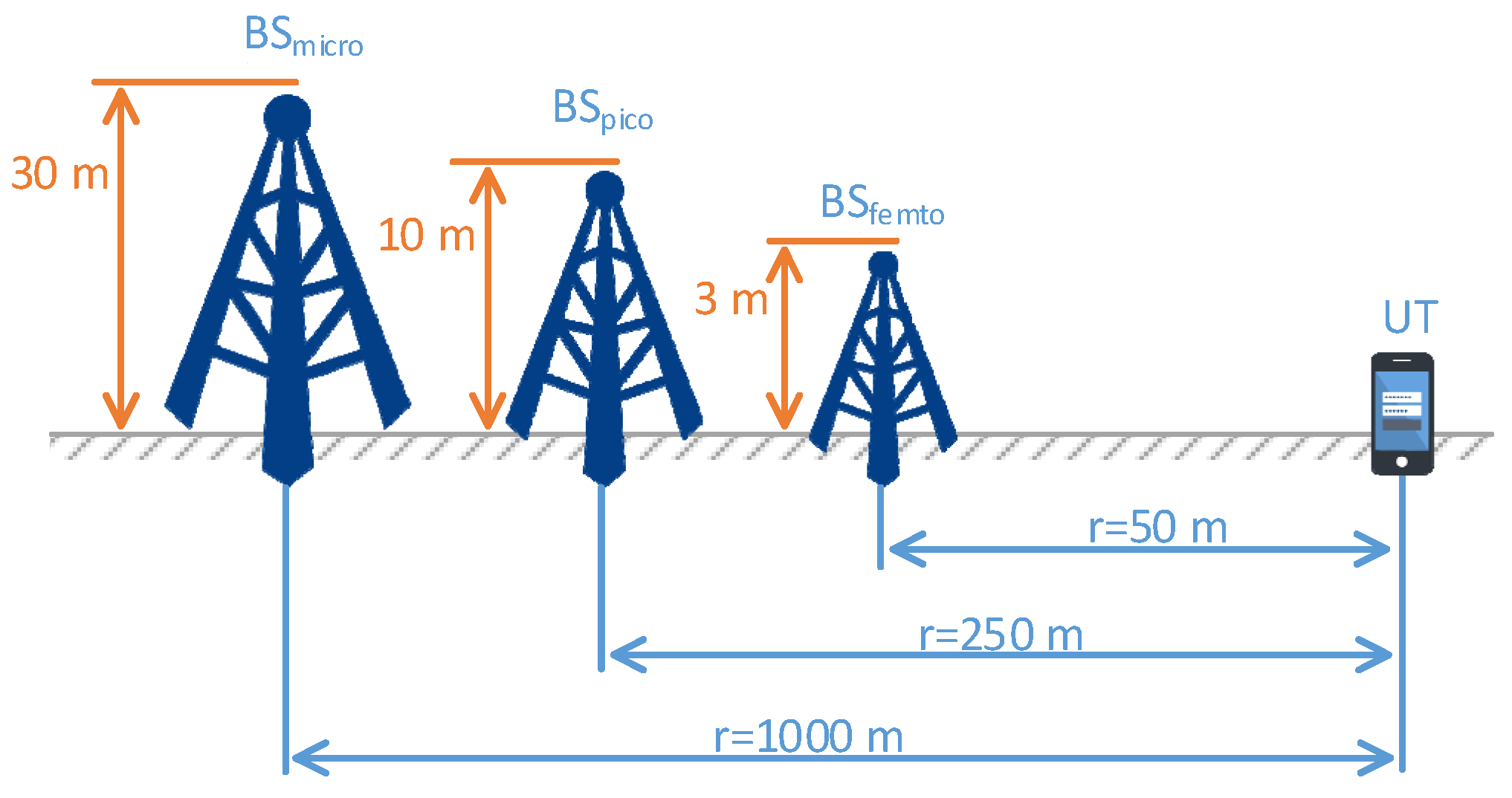
The UTs were placed at the cell edge, as shown in Figure 6.

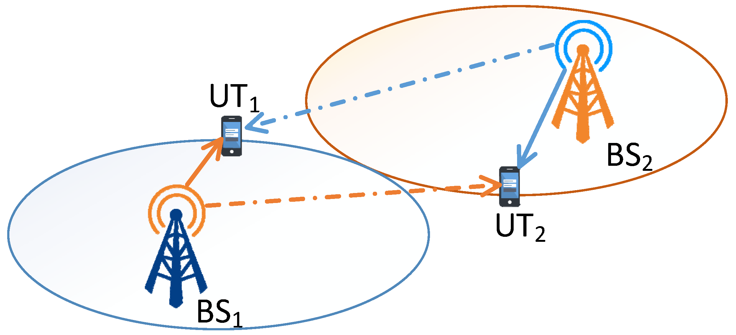
Two cases were considered: when the user was placed at the edge of the zone without interfering signal (LOS/NLOS scenarios) and with interfering signal (LOS/NLOS scenarios). The first included one BS and one UT. In scenarios with two BSs, the second BS₂ was located at a distance of 2r. Figure 7 shows the signal propagation model for the second case with two BSs and one UT.

3.1.3. Antenna Model

The receiving and transmitting antennas were simulated using the capabilities of QuaDRiGa. The main parameters of antenna elements were taken from TR 38.901, v16.1.0 [10]. The results presented below were obtained when implementing the MIMO 8 × 8 model using symmetrical antenna arrays in which antenna elements are located at the vertices of regular polygons [14].

3.1.4. Scenarios

When verifying the model and comparing the methods of calculating antenna weights, two known channel models were used: the mmMAGIC model and the channel model proposed in the 3GPP_TR38.901, based on WINNER [10].

The femtocell was simulated using 3GPP_38.901_Indoor and mmMAGIC_Indoor scenarios. These scenarios characterize the signal propagation environment inside buildings in the area up to 50 m. The height of BS antenna was 3 m, and for UTs it was 1–1.5 m. The femtocells are designed to expand cells in residential and corporate premises, unload the network and provide communication at any internal point of buildings.

To simulate a picocell, the following scenarios were used: mmMAGIC_UMi_O2I, mmMAGIC_UMi, 3GPP_38.901_UMi_O2I, 3GPP_38.901_UMi. These scenarios are normally used to model channels in a micro-urban environment to ensure both entirely external communication and data transfer from buildings to the external BS. The BS antenna was attached at the height of 10 m, and the UT at the height of 1–1.5 m. The cell radius of the BS was 200 m.

The microcell was described in scenarios 3GPP_38.901_UMa and 3GPP_38.901_RMa. The UMa scenario describes the macro-urban environment and the RMa scenario describes the rural environment. The height of the BS antenna was 25 m, the UT was 1.5 m high. The cell radius was 1 km.

More details about the main parameters of the scenarios are described in [3].

3.1.5. Calculation of Beamforming Vectors

The calculation of beamforming vectors was carried out with the two methods described above.

3.1.6. SNR/SINR Calculation

For cases with one BS, the SNR for the UT was calculated taking into account beamforming and using antenna coefficient vectors obtained with the first and second methods. The formula by which the calculation was performed is as follows:

$$SNR=\frac{\frac{P_{\mathrm{tx}}}{PL}\cdot G}{BW\cdot N_0},$$

(16)

where $P_{\mathrm{tx}}$ is the power of the BS transmitter, $PL$ is the path loss in the channel, G is the beamforming coefficient, $BW\cdot N_0$ is the internal noise of the UT.

For cases with multiple base stations, the interfering signal from the BS₂ was additionally taken into account, which was considered to be interference for the user. In this case, the SINR value was calculated using the following formula [11]:

$$SINR=\frac{\frac{P_{\mathrm{tx},11}}{P{L}_{11}}\cdot G_{11}}{\frac{P_{\mathrm{tx},22}}{P{L}_{21}}\cdot G_{21}+BW\cdot N_0},$$

(17)

where $P_{\mathrm{tx},11}$ is the transmission power of the BS₁, $P{L}_{11}$ is the path loss from the BS₁ to the UT₁, $G_{11}$ is the beamforming coefficient calculated for the BS₁ and the UT₁, $P_{\mathrm{tx},22}$ is the transmission power of the BS₂, $P{L}_{21}$ is the path loss from the BS₂ to the UT₁, $G_{21}$ is the beamforming coefficient calculated for the BS₂ and the UT₁.

3.2. Simulation Results

The simulation results for different scenarios are shown in

Table 2. Simulation results.

Scenario		NBS	PTX, dBm	5.8 GHz		28 GHz		68 GHz
				SNR/m1 dBm	SNR/m2 dBm	SNR/m1 dBm	SNR/m2 dBm	SNR/m1 dBm	SNR/m2 dBm
$\mathrm{Femtocell}, r$—50 m
LOS	mmMAGIC_Indoor	1	20	59.8	74.6	49.2	60.8	38.7	51.8
	3GPP_Indoor			56.3	69.3	44.6	55.6	36	46.9
NLOS	mmMAGIC_Indoor	1	20	27	43.1	9.2	20.9	1.1	13.6
	3GPP_Indoor			29.9	43.4	8.5	23.2	1.9	15.2
$\mathrm{Picocell}, r$—250 m
LOS	mmMAGIC_UMi_O2I	1	24	35.6	51.2	27.4	36.5	18.3	32.5
	mmMAGIC_UMi			38	52.9	25.3	39.7	23.9	31.3
	3GPP_UMi_O2I			35.4	46.6	25.5	35.9	20.9	27.4
	3GPP_UMi			39.3	52.8	30.4	38.9	25.9	31
NLOS	mmMAGIC_UMi_O2I	1	24	−22	−10	−16	−22.9	−40.4	−29.8
	mmMAGIC_UMi			−17.9	−6.8	−21.4	−18.8	−39.2	−25.1
	3GPP_UMi_O2I			12	23.5	−0.9	11.4	−21.6	−4.1
	3GPP_UMi			11	23.5	−1.4	5.7	−10.2	0.7
$\mathrm{Microcell}, r$—1000 m
LOS	3GPP_UMa_O2I	1	37	36.9	43.8	22.2	32.9	6.1	24.9
		2		23.4	33.7	7.5	24.4	6.3	15
	3GPP_UMa	1		32.1	44.4	25.3	40	24.6	33.5
		2		25.3	32.1	19.9	30.3	11.6	21.3
	3GPP_RMa_O2I	1		37.1	47.9	29.5	37	22.1	30.2
		2		32.9	38.9	12.3	24.5	12.9	21.7
	3GPP_RMa	1		37.2	49.6	30.9	42.3	26.8	34.3
		2		30.3	40.1	26.5	34	15.3	25
NLOS	3GPP_UMa_O2I	1	37	8.2	15.7	−9	1.1	−19	−4.8
		2		−1.4	9.8	−18	−5.7	−21.1	−11.2
	3GPP_UMa	1		10.4	21.9	−14.1	−5.5	−24.5	−12
		2		−0.6	13.3	−20.5	−14.6	−32.2	−19.8
	3GPP_RMa_O2I	1		−1.6	12.2	−8.4	−2.9	−20.8	−9.4
		2		−8.8	6.9	−17.3	−10.1	−28.6	−17.7
	3GPP_RMa	1		−2.1	5.8	−18.3	−8.9	−26	−16.8
		2		−9	−0.5	−25.5	−16.3	−33.4	−22.8

. This table shows the average SNR/SINR at the edge of the cell as shown in Figure 6 and Figure 7. The average SNR was determined from 50 model runs. SNR/SINR was calculated for two cases. In the first case, the beamforming coefficients were calculated by method 1. In the second case, the coefficients were calculated by method 2.

4. Discussion

In data communication systems, most characteristics are closely related to the SNR/SINR value. An increase or decrease in this parameter that characterizes the channel leads to a direct change in the parameters that characterize the system. In order to more clearly compare and characterize the scenarios presented in Table 2, it is much easier to use the channel throughput parameter rather than the SNR/SINR level. It is known that 5G is an adaptive system that adapts to changes in the channel. For this, the system supports multiple modulation and coding schemes (MCS) presented in [15]. The selected MCS mode affects the throughput. We used the research in [16] to relate SNR/SINR, MCS and throughput. In this paper, the authors mapped the SNR/SINR values to MCS and throughput.

When simulating a femtocell, the BS power was 20 dBm, according to the example given in [17]. When comparing the obtained data presented in Table 1 with [16], we found that, with LOS, data could be transmitted with the maximum MCS29 index for all frequencies. This provides a throughput of over 1.7 Gbps. The throughput already varies significantly depending on both the carrier frequency and the calculation method chosen for NLOS scenarios. The throughput value is reduced by 8.5 for the first calculation method for 68 GHz (MCS5–6), and by 2.2 for the second method (MSC16–18). Since the standard deviation of the SNR values in the simulation was about 9 dB, then for the second calculation method there are also values below 10 dBm for the frequency of 68 GHz. Therefore, to deploy internal networks at this frequency, a LOS is required in the room since various obstacles will lead to significant signal attenuation.

The BS power for picocell simulation was 24 dBm [17]. Picocells are characterized by scenarios of data transmission from the BS to the UT that is located both inside the building and in the external urban environment. For LOS scenarios, the throughput will decrease from 1.7 Gbps (MCS29) to 1.2–1.5 Gbps (MCS25–20) as the carrier frequency increases depending on the calculation method. For NLOS scenarios, the SNR value falls below the threshold for the 68 GHz frequency; for the 28 GHz frequency, the values allow you to get 150, 600 Mbps, for 5.8 GHz–600 Mbps, 1.4 Gbps for the first and second calculation methods, respectively.

A microcell base station has a power of 37 dBm [17]. At the same time, the SNR level above the minimum threshold for LOS and NLOS scenarios is retained only for the 5.8 GHz frequency range. The influence of signal interference on the SINR level was additionally checked in the case of two BSs in a microcell. In the presence of interference from the neighboring BS, the calculated SINR level decreased by, on average, 8 dBm. The throughput for 5.8 GHz in the case of the LOS scenario was 1.3–1.7 GHz, and for NLOS cases it was 414–676 Mbps for rural areas and 715–1037 Mbps for urban areas.

Comparing the two methods for calculating the antenna weight coefficients, we can conclude that the proposed method has an average gain of 10 dB in comparison with the one considered in article [2,11]. The model for each of the scenarios was run twice. The first time the antenna weights were calculated according to method 1, and the second time according to method 2. As a result, we compared the average signal power ratio for these cases. The results are presented in

Table 3. The ratio of the average power of the $P_{\mathrm{rx},\mathrm{m}2}$ (method 2) to the $P_{\mathrm{rx},\mathrm{m}1}$ (method 1).

Parameter	Femtocell	Picocell	Microcell
			No Interference	Interference
$P_{\mathrm{rx},\mathrm{m}2}/P_{\mathrm{rx},\mathrm{m}1}$, dB (LOS)	12.4	10.9	9.1	9.7
$P_{\mathrm{rx},\mathrm{m}2}/P_{\mathrm{rx},\mathrm{m}1}$, dB (NLOS)	13.6	11.3	9.9	10.1

.

5. Conclusions

Beamforming technology is an important part of 5G systems since they use higher frequency signals. From the conducted research, the obvious conclusion is that without beamforming, it is impossible to provide an acceptable signal power at the receiving side located at the cell edges at millimeter-wave frequencies. The lack of LOS for such frequencies is a problem and leads to a significant decrease in signal power of up to 30–40 dB.

The proposed method for calculating beamforming vectors has shown its effectiveness in comparison with the method proposed in [2]. The described model currently allows calculating the SNR/SINR level only for stationary scenarios, without using all the capabilities of QuaDRiGa. In the future, it is planned to implement a model that will take into account the UT movements, changes in scenarios over time, delays in the process of calculating antenna weight coefficients and the time spent on performing and transmitting the channel estimations. It is also planned to add algorithms for calculating weight coefficients based on incomplete knowledge of the transmission channel.

References

- List of 5G NR Networks. 2021. Available online: https://en.wikipedia.org/wiki/List_of_5G_NR_networks (accessed on 10 September 2021).
- Zhang, M.; Polese, M.; Mezzavilla, M.; Rangan, S.; Zorzi, M. ns-3 implementation of the 3GPP MIMO channel model for frequency spectrum above 6 GHz. In Proceedings of the Workshop on ns-3, Porto, Portugal, 13–14 June 2017. [Google Scholar]
- Jaeckel, S.; Raschkowski, L.; Börner, K.; Thiele, L. QuaDRiGa: A 3-D Multicell Channel Model with Time Evolution for Enabling Virtual Field Trials. IEEE Trans. Antennas Propag. 2014, 62, 3242–3256. [Google Scholar] [CrossRef]
- Jaeckel, S.; Börner, K.; Thiele, L.; Jungnickel, V. A Geometric Polarization Rotation Model for the 3D Spatial Channel Model. IEEE Trans. Antennas Propag. 2012, 60, 5966–5977. [Google Scholar] [CrossRef]
- QuaDRiGa. 2021. Available online: https://quadriga-channel-model.de (accessed on 10 September 2021).
- Ali, E.; Ismail, M.; Nordin, R.; Abdulah, N.F. Beamforming techniques for massive MIMO systems in 5G: Overview, classification, and trends for future research. Front. Inf. Technol. Electron. Eng. 2017, 18, 753–772. [Google Scholar] [CrossRef]
- Passoja, M. 5G NR: Massive MIMO and Beamforming–What Does It Mean and How Can I Measure it in the Field. 2018. Available online: https://www.rcrwireless.com/20180912/5g/5g-nr-massive-mimo-and-beamforming-what-does-it-mean-and-how-can-i-measure-it-in-the-field (accessed on 5 December 2021).
- Schwarz, S.; Rupp, M. Reliable Multi-Point Transmissions Over Directional MISO TWDP Fading Channels. IEEE Trans. Veh. Technol. 2021, 70, 1394–1409. [Google Scholar] [CrossRef]
- Maliatsos, K.; Bithas, P.S.; Kanatas, A.G. A Low-Complexity Reconfigurable Multi-Antenna Technique for Non-Terrestrial Networks. Front. Comms. Net 2021, 2, 696111. [Google Scholar] [CrossRef]
- 5G; Study on Channel Model for Frequencies from 0.5 to 100 GHz Release 14, Document TS 38.901, V.16.1.0, 3GPP. 2018. Available online: https://www.etsi.org/deliver/etsi_tr/138900_138999/138901/16.01.00_60/tr_138901v160100p.pdf (accessed on 27 September 2021).
- Mezzavilla, M.; Zhang, M.; Polese, M.; Ford, R.; Dutta, S.; Rangan, S.; Zorzi, M. End-to-end simulation of 5G mmWave networks. IEEE Commun. Surv. Tutor. 2018, 20, 2237–2263. [Google Scholar] [CrossRef]
- Borsdorf, R.; Higham, N.J.; Raydan, M. Computing a nearest correlation matrix with factor structure. SIAM J. Matrix Anal. Appl. 2010, 31, 2603–2622. [Google Scholar] [CrossRef] [Green Version]
- Biglieri, E.; Calderbank, R.; Constantinides, A.; Goldsmith, A.; Paulraj, A.; Poor, H.V. MIMO Wireless Communication; Cambridge University Press: Cambridge, UK, 2007; 323p. [Google Scholar]
- Harrison, C.W. Symmetrical antenna arrays. Proc. IRE 1945, 33, 892–896. [Google Scholar] [CrossRef]
- 5G; Physical Layer Procedures for Data Release 15, Document TS 38.214, V.15.3.0, 3GPP. 2018. Available online: https://www.etsi.org/deliver/etsi_ts/138200_138299/138214/15.03.00_60/ts_138214v150300p.pdf (accessed on 25 September 2021).
- Ramos, A.R.; Silva, B.C.; Lourenço, M.S.; Teixeira, E.B.; Velez, F.J. Mapping between Average SINR and Supported Throughput in 5G New Radio Small Cell Networks. In Proceedings of the 2019 22nd International Symposium on Wireless Personal Multimedia Communications (WPMC), Lisbon, Portugal, 24–27 November 2019. [Google Scholar]
- Kovalchukov, R.; Moltchanov, D.; Gaidamaka, Y.; Bobrikova, E. An accurate approximation of resource request distributions in millimeter wave 3GPP new radio systems. In Lecture Notes in Computer Science, Proceedings of the Internet of Things, Smart Spaces, and Next Generation Networks and Systems, St. Petersburg, Russia, 26–28 August 2019; Springer: Cham, Switzerland, 2019; pp. 572–585. [Google Scholar]
Figure 1.
Analog beamforming scheme.
Figure 2.
Digital beamforming scheme.
Figure 3.
Hybrid beamforming scheme.
Figure 4.
Block diagram of the model.
Figure 5.
Small cells.
Figure 6.
Layout of BSs and UTs for three cells.
Figure 7.
Signal propagation diagram with interfering signal.