
Nonlinear Problems of Equilibrium Charge State Transport in Hot Plasmas

National Research Centre “Kurchatov Institute”, P.O. Box 3402, Ploschad akademika Kurchatova 1, 123182 Moscow, Russia
Symmetry 2021, 13(2), 324; https://0-doi-org.brum.beds.ac.uk/10.3390/sym13020324
Submission received: 22 December 2020
/
Revised: 7 February 2021
/
Accepted: 10 February 2021
/
Published: 16 February 2021
(This article belongs to the Special Issue New Trends in Plasma Physics)
Abstract
:The general coupling between particle transport and ionization-recombination processes in hot plasma is considered on the key concept of equilibrium charge state (CS) transport. A theoretical interpretation of particle and CS transport is gained in terms of a two-dimensional (2D) Markovian stochastic (random) processes, a discrete 2D Fokker-Plank-Kolmogorov equation (in charge and space variables) and generalized 2D coronal equilibrium between atomic processes and particle transport. The basic tool for analysis of CS equilibrium and transport is the equilibrium cell (EC) (two states on charge and two on space), which presents simultaneously a unit phase volume, the characteristic scales (in space and time) of local equilibrium, and a comprehensive solution for the simplest nonlinear relations between transport and atomic processes. The space-time relationships between the equilibrium constant, transport rates, density distributions, and impurity confinement time are found. The subsequent direct calculation of the total and partial density profiles and the transport coefficients of argon impurity showed a strong dependence of the 2D CS equilibrium and transport on the atomic structure of ions. A model for recovering the recombination rate profiles of carbon impurity was developed basing on the CS equilibrium conditions, the derived relationships, the data about density profiles, plasma parameters and ionization rates.
1. Introduction
Understanding the behavior and control of impurities as an inevitable component of magnetically confined plasmas continue to be a topic of considerable importance in fusion research programs. Steady state mode of operation with impurity equilibrium is of vital to the success in modern experimental studies of improved confinement and stability of standard H-modes on tokamaks and stellarators [1,2].
In these devices, the radial transport of plasma particles across the magnetic field is accompanied by random change in their charge states (CS’s) due to ionization-recombination processes. The probabilistic imposition of these atomic processes on the transport of impurity particles occurs in an unusual phase space, which includes the discrete space of (Z + 1) CS’s. So, the resulting transport turns out to be at least two-dimensional (2D), while its structure involving an intersection of statistically independent processes is unexpectedly complicated. A consistent approach to this general 2D transport problem could suggest the use of multidimensional (mD) Fokker-Planck-Kolmogorov equation (FPKE) [3,4,5].
Meanwhile, for more than four decades, the description of impurity transport remained implicitly simplified and was reduced to a 1D diffusive-convective model (DCM), represented in 1D impurity transport codes (see, for example, the STRAHL code [6]). Here, the standard 1D continuity equation was supplemented in the right-hand side with also a standard 1D flux balance of ionization-recombination processes interpreted as random sources and sinks of charged particles. So, the required 2D description was just replaced by the sum of these 1D parts. The corresponding misinterpretation fell into an inevitable contradiction with the systematic approach that the theory of the generalized FPKE could provide. Indeed, the essential cross terms (mixed derivatives) representing the coupling of atomic processes with particle transport were also lost in the DCM equations. Moreover, the required discretization of these equations revealed and returned this 2D transport problem but only in the form of a 2D grid model (GM) in charge and radial variables (see discussion in [6] on page 6).
In the extensive practice of modeling medium and heavy impurities and with an increase in the rates of ionization-recombination it was found that the DCM sensitivity to the empirical transport remains extremely low [7,8,9,10,11,12,13] and just unacceptable for W impurity [14,15].
Nevertheless, the leading role in interpreting the behavior of impurities was assigned to various mechanisms of particle transport in the 6D phase space (of coordinates and velocities) in terms of the Boltzmann kinetic equation and its consequences carefully studied in the neoclassical transport theory [16]. But in the basic equations of neoclassical transport, the charge state as a mandatory variable was ignored along with impurity charge state space (see, e.g., Equation (2.2) in [16]).
A consistent critique of the standard 1D approach using DCM was recently given along with a completely new understanding of impurity transport in terms of the 2D CS transport [17]. The main unresolved physical problem outlined here was that 1D (radial) transport of particles would have to be clearly distinguished from the generalized 2D transport in the proper 2D phase space, where the particle transport is only part of CS transport. It is important, therefore, to make, first of all, a terminological distinction between particle and CS transports, that is, to introduce and develop the concept of CS transport. But the initial idea was to consider the role of ionization/recombination processes not as sources and sinks in the standard 1D transport equations, but on equal terms with particle transport, as a kind of transport phenomenon [18,19,20]. Due to mentioned imposition, the basic components of impurity transport turn out to be mixed according to probabilistic laws in a resulting generalized 2D transport. This understanding has been reformulated step by step in framework of traditional analysis via diffusive D and convective V coefficients in terms of CS transport [21,22] and finally allowed us to clarify the structure and probabilistic nature of impurity transport [17].
However, before any subsequent transition to equations describing the details of the distribution function with operators, the basic (first) principles for any subsequent analysis of the transport of charged particles are mandatory. Indeed, although, there is no particle without CS, as well as no CS of no particle, but there is a fundamental difference between the transport of particles and the transport of their CS’s due to ionization and recombination processes. In fact, let the probability of CS transport by particles be H(P), and by atomic processes be H(A), then the probability of events P + A is expressed, as is known, by the general Formula (1):
which shows that the generalized impurity transport includes three mandatory components: (i) CS transport by particles or p-transport, (ii) CS transport by atomic processes or a-transport, and, finally, (iii) CS transport represented by probabilistic intersection of a-transport and p-transport but irreducible to any of them. Note that the latter is the most represented case of events related to impurity transport in plasma. It is clear from Formula (1) that DCM is limited to analyzing only the first two components, implicitly (and erroneously) assuming that events P and A are incompatible.
Following the logic of Formula (1), the events caused by the intersection of and ensuring the local occurrence of any ion, are initially and in principle non-local, mixed by products of their probabilities in subsequent expressions, and as a result are indistinguishable due to the probabilistic nature and logic of the sum of P + A.
The significant advantage of the CS concept of impurity transport is the self-consistency of the developed 2D approach. The 2D Markovian impurity equilibrium directly provides the possibility to calculate D and V using the 2D FPKE adopted to the discrete CS phase space [17]. This makes it possible to perform transport studies without any additional empirical coefficients, while all components of 2D transport are expressed in more general way. The additional possibilities of the local (core and edge) transport studies also follow from the proposed 2D modelling.
From a theoretical point of view, we are faced here with a complex 2D structure of the impurity equilibrium and with its inevitable symmetry along with the possibility of the self-consistent determination of D and V. Moreover, the standard 1D descriptions of impurity ionization equilibrium or the stationary distribution (radial profiles) of the total impurity density is just included in this 2D model of Markovian equilibrium. We assume a 2D Markov equilibrium of impurities, since it follows from the so-called ergodic principle [3]. In this case, the CS transport of charged particles should be considered as an equilibrium transport. The transport rates are locally determined by a 2D probabilistic balance between the motion of impurity particles and the change in their charges due to atomic processes. In addition, the particle conservation law implied in the DCM equations is just generalized to the conservation of impurity CS moving in the 2D phase space. It is that results in a symmetric representation of transport in charge and radial variables on equal terms as suggested by the generalized FPKE.
Thus, the concept of impurity CS transport allows one to draw an unexpected conclusion about the determining role of atomic processes in impurity transport [17].
Clear evidence of this interpretation can be revealed in experiments and related modelling practice. First of all, this is a coronal equilibrium (CE) of heavy impurities indeed found in the early studies of Cr, Ni, and Mo impurities on the TFR tokamak [23,24], and then confirmed by modelling practice for W on the ASDEX Upgrade tokamak [14,15]. This meant that the equilibrium assumed by the DCM between 1D particle transport and 1D balance of ionization-recombination processes could not be observed, since in fact we are dealing here with the 2D equilibrium of the plasma impurity.
We further note the observations of a noticeable drop in the diffusion coefficient D at the central impurity accumulation and a sharp difference in transport in the plasma core from transport in the rest periphery (see, for example, [25]). These results can be explained by the largest size of the central equilibrium cell (CEC), as clearly seen from the CS transport modelling [17].
The next important experimental evidence is the known coupling found between central accumulation of impurities and diffusion coefficient D: the greater the accumulation of the impurity in the plasma core, the lower D [17,26], and vice versa, that is, the “flat” distribution is systematically associated with an increase D to anomalous values (in the conventional comparison with neoclassical predictions) from the core to the plasma edge.
Finally, there are also two characteristic maxima on the total density profiles. The observed impurity accumulation takes place simultaneously at the edge and in the plasma core, as found, e.g., for W in JET [1] that consistently reproduced in the CS transport model [17].
Meanwhile, the 2D imposition of ionization/recombination on the particle transport results in a fundamental nonlinearity of the 2D transport analysis, which aim is to find and study the particle transport. The setting of the problem cannot be reduced only to the standard 1D linear equations in principle. A more general 2D problem consists in directly modeling the impurity density profiles (both partial and complete) observed in experiments to find the corresponding D and V, using only the atomic database of ionization/recombination rate coefficients, as shown in [17].
However, this 2D analysis gives the nonlinear equations for even a simplest 2D system of four charge states (two in space and two in charge called the equilibrium cell (EC))—leads to a transcendental equation [17]. The general solution was developed basing on a number of reducing 2D schemes and the use of the pseudo-state technique. Thus, the solution of the nonlinear transport problem is represented by two main stages: first, by reducing the general discrete GM of impurity equilibrium to a set of local equilibrium cells and, second, by finding their transport coefficients that provide the calculation of density profiles along with the transport coefficients.
Nevertheless, such direct modelling of the total density profiles suffers from the problems associated with the usual and significant uncertainties of atomic rates. As well known, the most uncertainties appear in the data of cx- and dielectronic recombination rates [8,14,15].
To solve this uncertainty problem, in this paper we propose a new formulation of the transport nonlinear problem along with the developing CS transport model. It is based on the possibility of analyzing the equilibrium transport by separating its absolute and relative scales, which represent the equilibrium constant λ and the corresponding rate ratios [17]. Then, the input data in this model are the typical radial profiles of the total impurity density observed in experiments and ionization rate coefficients. So, we continue here the previous analysis of the CS equilibrium with its absolute scale, λ, which turns out to be common to all emerging nonlinear problems [17].
We further show that an important relationship can be established between λ, the standard transport coefficients and the impurity confinement time . A generalization of the EC concept is developed in the form of the reduced equilibrium cell (REC). The REC concept allows us to proceed directly to impurity equilibrium analysis based on a wide variety of the density profiles as mentioned above.
The structure of the paper is as follows: In the second part, we consider the symmetry features of the basic equations of the CS equilibrium and transport, analyzing from this point of view the same basic formulas obtained earlier in [17]. An extended set of possible schemes for reducing GM to easily analyzed simplifications is presented, also taking into account possible symmetries of the proposed approach. The matrix description of the impurity density profiles is developed and its important relationship with the GM equilibrium is shown through the important scale factor λ. Its dependence on the atomic structure of the impurity ions, the most abundant in plasma, is analyzed in detail in Section 3. The novel CS model and the basic results of recovery of the relative density profile of hydrogen neutrals that determine the impurity charge exchange recombination rate are given in Section 4. Section 5 presents the conclusions.
2. Charge State Equilibrium and Transport
In the classical review of Braginsky [27], an equation representing the impurity transport was given as follows Equation (2):
where is the density of impurity particles in k-th CS (k = 0, 1,..., Z), is the particle flux of the k-th CS and . All changes of due to ionization-recombination processes are described in Equation (2) by the term , but the expression for it was not considered in the review. Nevertheless, it is clearly seen, that the proper phase space for Equation (2) has two independent variables, k and r (and time). Consequently, it would have to be considered in the 2D phase space of these k and r on equal terms using the system approach suggested by FPKE. In this case, the 2D transport represented in Set (2) must also be consistently analyzed in a general series of discrete mD Markovian processes.
2.1. The Discrete Transport and Equilibrium Conditions
In the general mD case, the differential probability distribution function with independent variables can be represented by the FPKE [3,4,5], shown as Equation (3):
where is a vector of convective fluxes, is a tensor of generalized coefficients of diffusion in the mD phase space, . It is also assumed here that the variables xi and xj are changed almost continuously. The function must satisfy the Smoluchowski Equation with integration over mD phase volume . The derivation of Equation (3) can be found elsewhere [4,5].
in Equation (2) can be generally found from comparing Equations (2) and (3). The mixed derivatives included in the resulting expression in the 2D case of interest are related to the volume , which is directly given in these derivatives and just not present in the standard DCM. (see, Equation (2.2) in [16]). It should be noted that the mandatory integration of the general (mD) form of the kinetic equation on velocities to derive Equations (2) or (3) cannot, in principle, eliminate the differentials of variables with their product, , that determines the unit phase volume. Their spatial scale represents the non-locality of the 2D coupling between a- and p-transports in the EC. Therefore, if the conventional 1D equation does not contain them, then it follows that it contradicts and does not agree with both Formula (1) and the mD FPKE (3).
To represent atomic processes in convenient discrete form, Equations (2) and (3) must obviously be modified. Consider the discrete 2D GM, which is usually used to discretize Equation (2) in transport codes [6]. We introduce a grid probability distribution function, , where k = 0, 1, 2, ..., Z and n is the radial index instead of r; n = 1, 2, ..., N, N = m + 1, where m is the number of cells. Since is normalized as follows , we get , that is, the total local (on n) normalized particle density and , that is, the total normalized density of all ions with the same charge k. and are related to by the distribution functions and according to Equation (4):
and normalizations: , .
The CS dynamics on the grid are considered as the random jumps to neighboring positions (grid nodes): by k due to a-transport and/or by n due to p-transport. The a-transport rates are and , that is, the total rates of ionization and recombination. The p-transport rates (also in s−1) could be denoted as if the CS motion by p-transport is directed from n to n + 1 and as if the motion is directed from n + 1 to n. Note that these introduced transport coefficients are just a modified form of the conventional D and V and present the same, albeit unidirectional, particle fluxes. So, for rough numerical estimates, D and V could be obtained from these 1D matrix coefficients simply as and for the most abundant k states (see in detail in [28]).
The discrete 2D form of Equation (3) assumes the choice of the necessary system of pairwise incompatible events (in accordance with the general probability summation formula) associated with states without matching indices. Therefore, we consider pairs of diagonally conjugate states: (k, n) and (k + 1, n + 1); (k + 1, n) and (k, n + 1) and the corresponding diagonal rates and . Then the 2D equation (for example, for the first of the symmetric pairs) is obtained as Equation (5):
where the rate matrix is tridiagonal, Jacobian, singular (it has zero value in the spectrum of its real eigenvalues) and similar to some symmetric real matrix. At any time, t, of the temporal evolution of Equation (5), there is an ergodic limit (see [3]), which is determined by a complete set of these matrices. The stationary solution of Equation (5) is simultaneously the local equilibrium condition, shown as Equation (6):
The 2D equilibrium is symmetric, assuming the equalities of symmetric pairs of counter CS fluxes. Shown as Equation (7):
which can be proved strictly in general for any 2D structures (see in [17]). Therefore, note, that Equation (6) directly follow from these Equation (7) and independent of Equation (5).
The nonlinearity of the problems that arise in the analysis of the CS transport is directly follows from Equations (6) and (7), so we get Equation (8):
where and are arbitrary constants to be found. By defining Equation (9):
we obtain the general case of conditions (6) expressed in terms of products of conditional probabilities of particle and charge transport processes. Formally, using the normalization of with Equations (8) and (9), we obtain the set of rate equations. But even simplest expressions for the diagonal CS transport in the single EC give a strong nonlinear relationship between the probability distribution and transport rates (see, e.g., Equation (13) below or Equation (21) in [17]).
Thus, the rates and , are related in a nonlinear way to in accordance with Equations (1) and (5)–(9). Using Equation (4), Equality (7) can be rewritten as Equation (10):
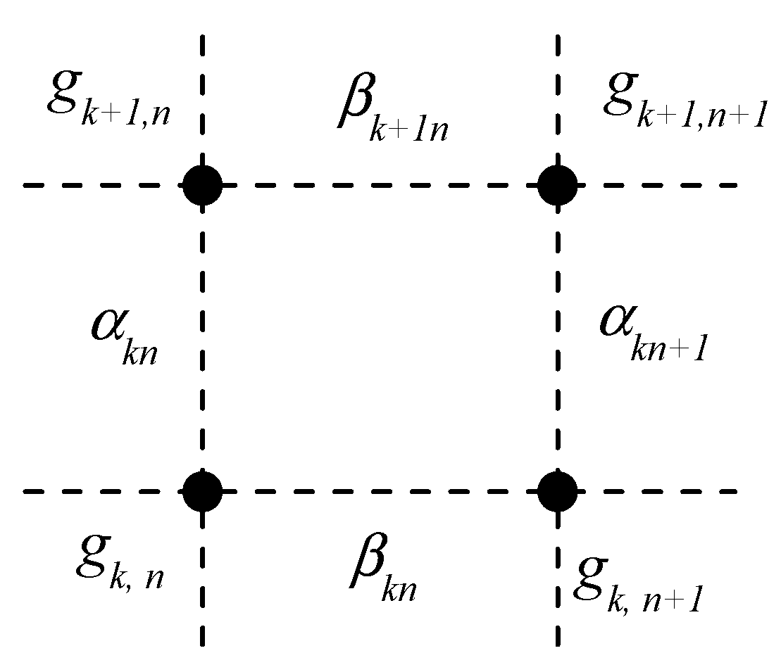
where both distribution functions are normalized (see after Equation (4)), hence Set (10) can be interpreted as a generalized equilibrium or double coronal equilibrium (DCE). For each cell, there are symmetric pairs of such equalities that define the local DCE conditions. A local unit of phase volume has a pair of necessary transport ratios, shown in Figure 1.
Each impurity particle within a local unit of the discrete phase space is characterized by four states. Consider the relationships: and . Using the entered relations, the Equations (7) and (10) can be rewritten again in the form of Equation (11):
where both values in the left part obviously depend only on the rates of ionization and recombination and relate only to a-transport, while in the right part—only to p-transport. Equation (11) defines the impurity equilibrium as the necessary local coupling of a- and p-transports, but within the size of each cell. A transport that satisfies the condition (11) could be called an equilibrium transport.
Whatever the mechanisms of p-transport in the plasma (collisional or turbulent), local equilibrium of impurities can only be provided by the equilibrium p-transport rates. Consequently, the local equilibrium transport is determined by statistically independent rates of ionization and recombination. Since the p-transport corresponds to the a-transport, that is, it turns out to be equilibrium, a generalized DCE of impurity (10–11) occurs.
Thus, local EC is simultaneously: (i) a unit phase space volume and the characteristic scale of the local equilibrium, (ii) self-consistent equilibrium system, which provides a comprehensive analysis of the rate ratios of a- and p-transports, (iii) a crucial tool for analyzing a general equilibrium of impurity CS transport.
Moreover, we argue that there is a fundamental difference in the basic estimates of the impurity equilibrium in the 1D and 2D cases. In contrast to the 1D case, 2D equilibrium relations are established between the fluxes of the same type of processes in each 2D cell (see Equations (7) and (10)) and, in addition, the relations of the relations themselves, as follows from (11). Mixed equilibrium fluxes (see, Equations (8) and (10)), which are the superposition of a-and p-transports, occur only in symmetric diagonal directions with inevitable nonlocal coupling. A similar mixture of atomic processes and particle transport was first derived from the 2D solution of standard equations [20,21].
The radial scale of the nonlocal coupling between particle transport and ionization/recombination is determined by the m value, that is by the local scale of the EC. The largest one is related to the CEC.
Equation (11) couples only the rate ratios, which can be reproduced for impurities with different Z and with significantly different rates. But only they determine the equilibrium transport along with the resulting stationary density distributions. The corresponding similarities of the equilibrium rate ratios can be suspected in experiments, e.g., when there is an apparently similar stationary density profiles of the central accumulation of C [29,30], Ar [31,32] and W [1,33].
Contrary, the absolute values of the atomic rates determine the equilibrium scale, λ, that is, an equilibrium constant of steady state impurity [17]. It turns out to be the same to all cells and reducing GM schemes, as will be shown below. Therefore, the difference in the equilibrium of impurities appears primarily as a function λ(Z), which strongly depends on the atomic structure and the rates of the most abundant ions. For light and mid-Z impurities, these are K- and L-shells of H-, He- and Li-like ions. Normalizing the atomic rates by this λ allows us to develop a generalized elementary 2D model of equilibrium that could be called a reduced equilibrium cell (REC). Formally the REC is just a special case of the EC with λ = 1.
2.2. Reduced Equilibrium Cell
The CS equilibrium and transport in the EC introduced elsewhere [17] is completely determined by the rates of ionization and recombination processes, , and , respectively. The relations , , , , , are either directly obtained from the given rates of atomic processes, or can be obtained from the equilibrium analysis. In particular, in the case of the EC the Equation (11) is presented in Equation (12):
Solutions of the equations describing the temporal evolution of densities , , , (for short, the subscripts for pairs are changed) include non-zero eigenvalues of the EC matrix equations. As was shown in the EC analysis [17], these turn out to be equal, i.e., , where , are the constants of the diagonal balance as follows from the FPKE adopted for the EC, , where , , and , where and .
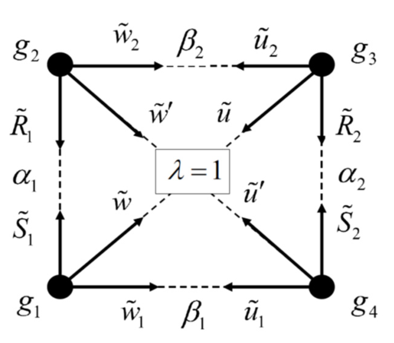
Now consider the REC, in which, as noted above, all rates are normalized to λ, that is, , , and . We also get that , and , . However, , , and remain the same. In this case, the definition of the REC is a set of equalities . The REC scheme is shown in Figure 2.
The basic equations derived for the EC are the same for the REC also, as shown in Equation (13):
where , in the notations , , , and (), ().
For the REC analysis we add to Equation (13) two expressions for and (where ) taken from the equation and the relation in the form of Equation (14):
The final equation, which is obtained from Set (13–14), has the form of Equation (15):
where the values are assumed to be given. Equation (15) differs from that for the EC [17], shown in Equation (16):
which can be resolved with respect to for a given , . An equilibrium with a given ionization base of the cell, s, could be called an S-equilibrium.
The symmetric version of the EC with subsequent R-equilibrium can be based on recombination processes (for given and ). This R-equilibrium is given by a triple with other version of final Equation (17):
It is important to note that the solution of Equations (15)–(17) is not a continuous function, since in general there are two equilibrium regions defined by inequalities (18):
and Equation (19):
The transition between regions (18) and (19) occurs in jumps in p, x and [17] at the bifurcation points of Equations (15)–(17). These points are the boundaries of the regions (18) and (19).
For other elementary equilibrium schemes involving one or more cells, the solutions of the final Equations (16) and (17) coincide in principle. However, real impurity equilibrium systems in a plasma with different equilibrium bases (s or in S- or R-equilibrium respectively) can differ significantly by their equilibrium rate profiles and by the conditions that implement the equilibrium at the variable boundaries. The point is that any of the three options is possible: (i) when the equilibrium can have both equilibrium bases and different profiles, (ii) when only one of the two equilibrium options is realized, and, finally, (iii) when there is no equilibrium for given distributions of parameters. Thus, the modelling shows that the complex cases turn out to have different equilibrium bases and respective boundary conditions.
Thus, the solution of Equation (15) can be used to model the CS equilibrium, which exactly corresponds to the given (or known from experiments) profiles of the total impurity density with known ionization rates. The modelling using this approach are considered below. However, unlike the settings of the direct Equations (16) and (17), which provide the calculated scale λ, the problem (15) assumes that λ is known in advance, e.g., from approximate estimates (which are discussed below) or from a preliminary approximate or direct calculation of the equilibrium.
Direct calculations of the equilibrium of the Ar impurity in the JET tokamak showed [17] that the last cell in the CCs differ from the others in a number of important properties. So, for m-th cell we get in the region (19). We also obtain that >>1, s >> 1, << 1. Typical values are γ = 20–100, s = 4–20, = . In this case, the analysis can be simplified and, in fact, gives the position of the impurity equilibrium boundary. In the region (19), it turns out that , , .
Further, the analysis of the equilibrium in the last EC allows us to calculate the limit values of the boundary densities that satisfy the simple criterion for several values of γ as a function . Figure 3 shows the dependence of the limit ratio of densities in the last EC. The equilibrium for a denoted value γ is possible only at densities higher than the calculated limit values.
2.3. Reduction Schemes
The Markovian equilibrium, assumed in GM for stationary plasma conditions, allows us to find the equilibrium transport by reducing GM by the pseudo-state technique. The main reducing schemes are shown in Figure 4.
The most obvious reduction options are local summations of the initial grid distribution function for each n and for each k. It is easy to find several reducing schemes where the nodes are convenient simple sums of CS’s that preserve the original density distribution with the normalization. Thus, the formal algebraic procedure allows to reduce the analysis of nonlinear rate transport equations to the solution of the transcendental Equations (15)–(17). So, the GM equilibrium can be successively reduced to a local equilibrium of just four pseudo-states of EC, which are the sums of the corresponding GM quadrants around the single nodes of local EC, that is , where i = 1, 2, 3, 4 with normalization preserved .
Invariance of the resulting distributions can be illustrated by comparing densities, for example, in simple schemes HL, EC, and SP, where they are connected by obvious equalities shown in Equation (20):
So, for the CCs and HL, the density distribution is common, i.e., a reduction invariant. In the same way, the horizontal (HL) and vertical (VL) lines of pseudo-states preserve and distributions, which are shared with the original GM (see Equations (3) and (4)). Summation of Equation (5) results in the following set of the HL shown in Equation (21):
where and , but for the VL to a similar set, shown in Equation (22):
where and .
Another important invariant of the reduction is the CS fluxes between the original neighboring states and their reducing pseudo-states. In this case, the changed transition rates between all new nodes must correspond to the pseudo-state densities. The equalities of probabilistic fluxes determine these rates between pseudo-states. The SP and EC rates are related to each other as follows Equation (23):
Obviously, in the case of the CCs scheme, the proper equilibrium is generally provided by the correct choice of the j and j + 1 levels of ionic charge k. It is seen that the choice is determined by the most abundant impurity ions in the plasma, i.e., their corresponding charge and external atomic levels. These j and j + 1 could be called the equilibrium levels of steady state impurity.
The first stage of the GM reduction to the CCs is the summation along vertical lines below and above the levels respectively. The resulting CCs pseudo-states are the following sums Equation (24):
The fluxes between levels in the original and reducing schemes are assumed to remain unchanged, which allows us to find the rates, shown in Equation (25):
The sequence of the ratios derived from the Equations (24) and (25) can be called the equilibrium function, shown in Equation (26):
which determines and similarly the function , since Equation (27):
Besides the density distribution and CS fluxes between neighboring states of original scheme there is another important reduction invariant. It is the equilibrium constant λ discussed in detail in the next section.
3. Equilibrium Constant
The reduction invariants allow us to obtain a general solution to the original transport nonlinear problem. But there is a common for all reducing schemes and, therefore, the most important equilibrium invariant given by the value λ, which should be considered in detail.
Averaging the atomic rates and its ratios over the corresponding φ functions for the n-th reducing EC and for levels of CCs, we get Equation (28):
It is seen that and remain the same for all reducing cells of the CCs. Then the sum in Equation (29):
is also a common constant. The same conclusions can be drawn in the symmetric case, shown in Equation (30):
The intersection of vertical and horizontal reducing lines and imposed of the EC’s (with the corresponding pairs of n and k) reveals that for any reducing local EC there is only a single common constant . Note that the non-zero eigenvalues of all reducing SP are also equal to λ. In other words, λ is a constant, that determines all possible cases of impurity equilibrium in GM.
The important relationship between λ and the equilibrium transport rates, density distributions, , and, finally, the characteristic times of the impurity confinement, , can be found as follows.
3.1. Time Scale of Transport Rates
In the case of steady state equilibrium (), the solution of Equation (21) is determined by the equalities of the same particle fluxes from neighboring pseudo-states and between them. Comparing these fluxes for HL and SP and using equation , we get the equalities corresponding to the conservation of fluxes for each pair of n and n + 1 states of HL and the sequence of SP pseudo-states, shown in Equation (31):
that gives a complete set of equations. The solution is expressed by Formula (32):
where and are the reduced particle transport rates shown by Formula (33):
Using Formula (32), Equation (25) can be rewritten as Equation (34)
where N is the matrix of Equation (25), is the reduced matrix combined from the values (33), shown in Formula (35)
where is the spectrum of its absolute eigenvalues (let ), determined by the density profile according to Equation (33), the matrix B is diagonal, and T is orthogonal, and Tt is the transposed orthogonal matrix (see, e.g., in [20]).
Thus, the value λ determines the scale of temporal evolution . The eigenvalues of is related only to the stationary profile , as follows from Equations (33)–(35).
3.2. Impurity Equilibrium and Transport Coefficients
The discrete structure of CS transport, finite equilibrium regions, and bifurcations during transitions between them strongly limit the possibility of describing impurity transport by differential equations that require continuity of the corresponding functions along with their derivatives in the entire domain of definition. On the contrary, the proposed matrix approach uses a minimum of input information to analysis and most closely corresponds to the physical nature of probabilistic (random) CS transport. Indeed, Equations (21) and (34) represent a matrix analogue of the standard 1D continuity equation for the total impurity density shown in Equation (36):
where . Note that for a stationary impurity profile obtained in experiment, the corresponding discrete profile is also well known, since , where , is the minor radius of the plasma column. Next, we note that in the accepted cylindrical geometry, it is convenient to set in accordance with Equation (21), and then . Comparing the coefficients before the second derivatives in Equation (21) (after expanding by n as a continuous parameter, see, e.g., in [17]) and (36) and using the Equation (32), we obtain the particle diffusion coefficient, D, in Formula (37):
where is a reduced diffusivity, which is easily calculated using Equation (33). The reduced convective velocity, , is obtained by a standard way .
The strong dependence occurs in Equation (37) for several reasons. First, using the expansion in series on n of Equation (21) we get the second derivative depending on n with corresponding coefficient (see, e.g., in [17,18,19,20]). Second, the comparison can only be made using the initially accepted cylindrical coordinate system with argument , which provides a correct description of the radial states (layers) with equal plasma volumes. Third, unlike Equation (36), the Equations (21) and (34) are linear on n. But the argument appears before the second derivative in the steady state solution of Equation (36), that is, in the confluent hypergeometric equation to be solved (see, for example, in [22,34,35,36]). Then, to convert the original coefficient before second derivative of linear Equation (21) into that of the standard Equation (36) with that required , it is necessary to include the correcting scale factor into the expression of D, since the factor is just included in the diffusivity profile .
Now we can directly calculate the reduced transport profiles and together with the profiles and corresponding to the given profile . We can directly derive and , and using the invariance of pseudo-state fluxes of HL and EC systems shown in Formulas (38):
where for each n we can use the following obvious expressions, shown in Formulas (39) and (40):
then from Equations (13) and (38)–(40) we get the relations of the HL and EC values shown by Expressions (41):
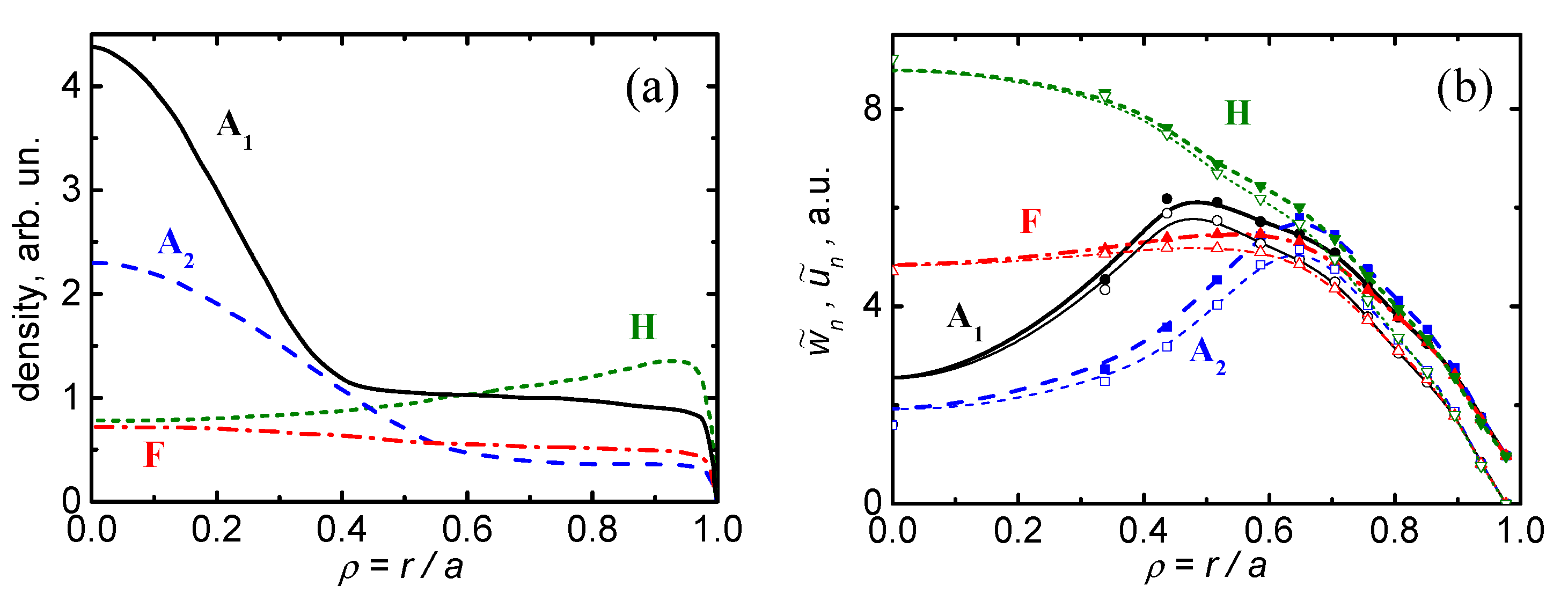
Typical profiles , for example, of C and Ar are well known from experiments (see, e.g., in [29,30,31,32,33,34]). The profiles can be (i) peaked in the plasma core, (ii) almost flat, or (iii) slightly hollow. Figure 5a shows these typical profiles observed in experiments, and Figure 5b shows the corresponding profiles and calculated on Equation (33).
Numerically and close to each other in almost the entire profile. So, we conclude that (see Equation (37)). The closer to the center of the plasma, the better the approximate ratio is reproduced. The profiles A1 and A2 with central accumulation correspond to a decrease in D in the plasma core, which is in qualitative agreement with the experiments [26] and modelling [17].
3.3. Impurity Equilibrium and Confinement Time
The confinement time of impurity particles, , is conventionally determined by the smallest of the eigenvalues of the divergence operator [34,35], which represents the particle transport in the standard Equation (36). In the proposed matrix case, the analogue of this value, as follows from Equations (34) and (35), is the product . We denote the smallest (non-zero) absolute eigenvalue of the spectrum of the matrix (see explanation to Formula (35)). Then can be found from the spectral decomposition of the matrix constructed by Formulas (32) and (33). Using this matrix approach, we obtain a relationship between and m. Figure 6 shows the calculations of these dependencies for the profiles shown in Figure 5a.
From the definition of , Equations (34) and (35) and calculations shown in Figure 6, we get Formula (42):
where the last approximate ratio is performed within a good accuracy, especially for flat (F) density profiles. From the expressions (37) and (42) we conclude that . The resulting estimates of the value for the various cases of equilibrium of C and Ar impurities are presented below.
3.4. Types of Impurity CS Equilibrium
The atomic structure of impurity ions is directly manifested in their CS equilibrium. It follows from Formulas (28) and (29) that changes in the equilibrium levels can affect both λ and . An additional factor here is, as mentioned above, the type of the equilibrium base—ionization (S) or recombination (R). This can be shown by modelling of impurity equilibrium.
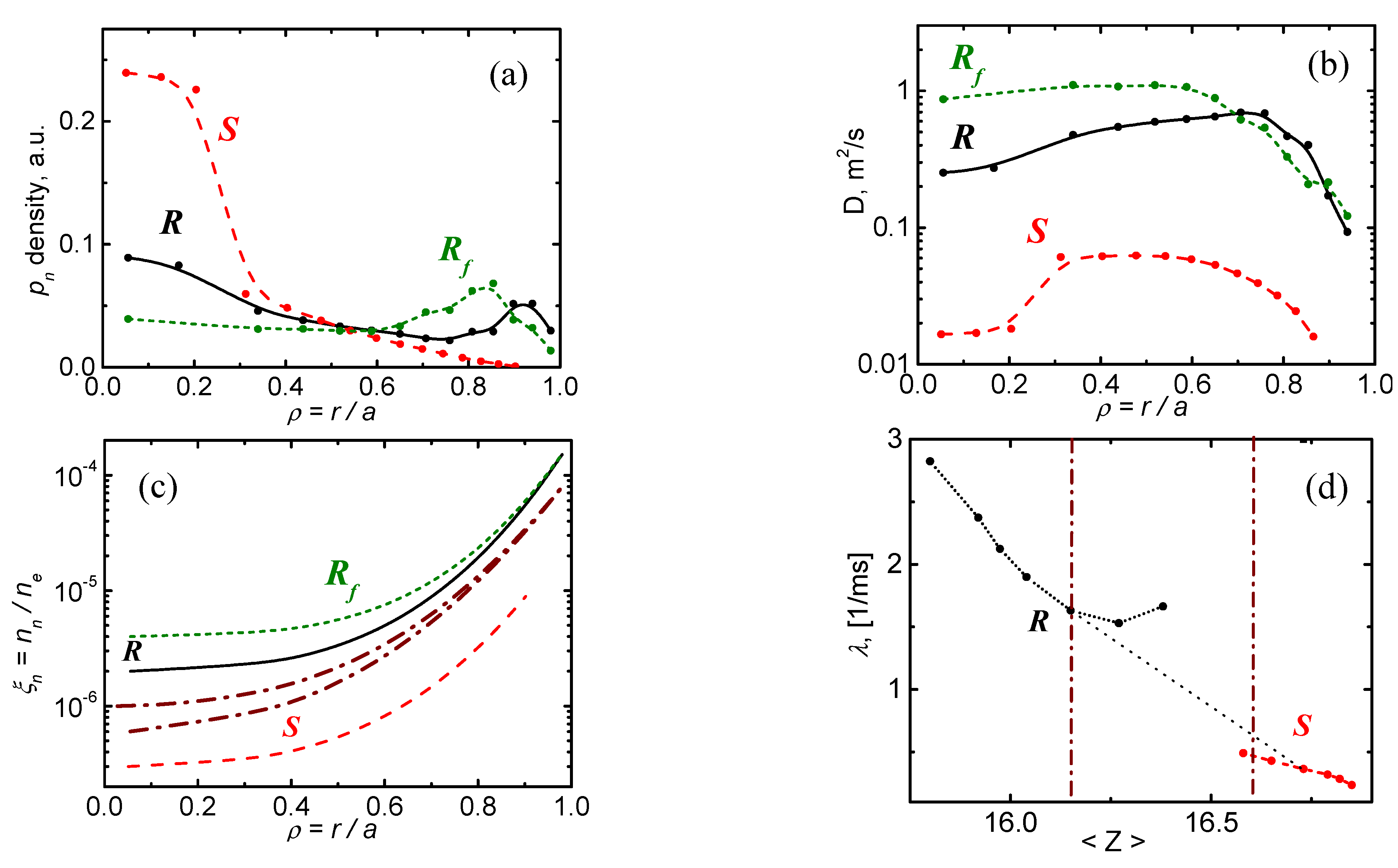
Figure 7 shows calculations (by the TICS code [17]) of the argon impurity equilibrium for the temperature and density profiles typical for a variety of discharge conditions in JET [31,32,34], in particular, for a plasma with keV, keV, and 4.5 × 10¹⁹ m−3. The selected profiles of temperatures, electron density, and relative density of hydrogen neutrals remain the same as previously used for modeling Ar transport in JET.
Figure 7a shows the profiles of the total argon density for three typical cases of the equilibrium observed in experiments. Here, discrete data points are connected by splines. The first profile, denoted by S, is a strongly peaked and obtained in the case of S-equilibrium with the base for He/H—like ions. The next profile denoted by R has two maxima (at the center and at the edge), calculated for R-equilibrium with the base for He/Li—like ions. Finally, that denoted by Rf, calculated for almost flat in the core and peaked at the plasma edge, also related to R-equilibrium (with He/Li—like ions). The calculations shown in Figure 7b show that a change of the levels He/Li (in R-equilibrium) to He/H (in S-equilibrium) leads to a significant decrease in D. This is obviously due to the low ionization and recombination rates of He-like and H-like ions.
Figure 7c shows the profiles that determine the rate profiles of recombination through charge-exchange of impurity ions on hydrogen neutrals and, hence, their corresponding equilibrium functions (26). Two regions of these equilibrium profiles for S-equilibrium (He/H) and for R-equilibrium (He/Li) are separated from each other by a narrow transition region depending on the plasma parameters that provide equilibrium. The gradual transition of impurity from R-equilibrium to S-equilibrium related to an increase in the average charge .
This transition requires a noticeable decrease in the charge-exchange rates across the entire plasma cross-section, and especially at the periphery. Even small fluctuations in the plasma parameters (e.g., ) at the equilibrium boundary can cause a transition between the S- and R-equilibrium regions along with a significant change in the values of D and . But since this is a transition from the regions (18) and (19), it can only occur in a jump. Figure 7d shows how the corresponding changes in λ occurs when trying to gradually vary the parameters of CS equilibrium.
The modeling calculations of CS equilibrium of Ar were performed for a variety of , and profiles close to the modelled [17] conditions at JET [31,32,34]. Thus, the studied CS equilibrium of the types discussed above can be represented in a very wide range of plasma parameters, revealing the corresponding range of λ and .
Figure 8 summarizes these variations of equilibrium values λ (a) and (b) caused by the change in the temperatures and from 1.5 to 8 keV and by the corresponding (to equilibrium) variations of (from the core to the equilibrium boundary) at an almost constant plasma density profile with . Full symbols correspond to S-, and open symbols to R-equilibrium type. The growth of leads to a noticeable increase in λ along with the increase . Increase changes a lot , but it does not change much , since . An increase in results in an increase , that is, to a shift of the obtained points on Figure 8 to the right. Figure 8b shows the corresponding calculations of on Formula (42).
These estimations of generally correspond to the measurements and known scaling for L-, I- and H-modes [38,39]. In particular, the estimates ms for = 15/16 (Li- and He- like Ar) (see in Figure 8b) turn out to be in good agreement with scaling for L-mode plasmas [38] and for I-mode in Alcator C-Mode [39], but taking into account its higher plasma density , since . Moreover, the calculated dependence clearly shows the same tendency of slow decreasing with strongly increase in from 1.5 up to 4 keV (see, e.g., Figure 4 in [39]). The transition from L- to H-mode plasmas results in a stepwise increase in ms [38,39,40,41] and corresponds to impurity equilibrium (both S- and R-type) for higher levels = 16/17 (He- and H- like Ar) and = 17/18 (H-like and full stripped Ar ions).
3.5. The Radial Scale of the CS Equilibrium
As follows from Formulas (37) and (42), the radial number of equilibrium cells m plays a significant role in the scale factors of the impurity CS transport. The number of radial cells m was initially determined by the number of times on average the particle changes its CS moving from the center to the grid boundary. However, there is an inevitable contribution in m of the other transport processes. Therefore, it is not entirely clear how m is defined. Indeed, it could be assumed that collisional and/or turbulent transport in the plasma can contribute to m along with atomic processes, e.g., as a simple sum . The simulations of the CS equilibrium transport show that it is necessary for C, for Ar and for W. But for C, the largest excess over the reasonable estimates ( at least) is obtained, whereas for medium and heavy impurities, it can be assumed that . It is also worth noting that . But in accordance with Formula (42) . So, if we assume that , then from , we can finally get a slowly decreasing dependence as observed in experiments with light impurities (see, e.g., in [12,42]).
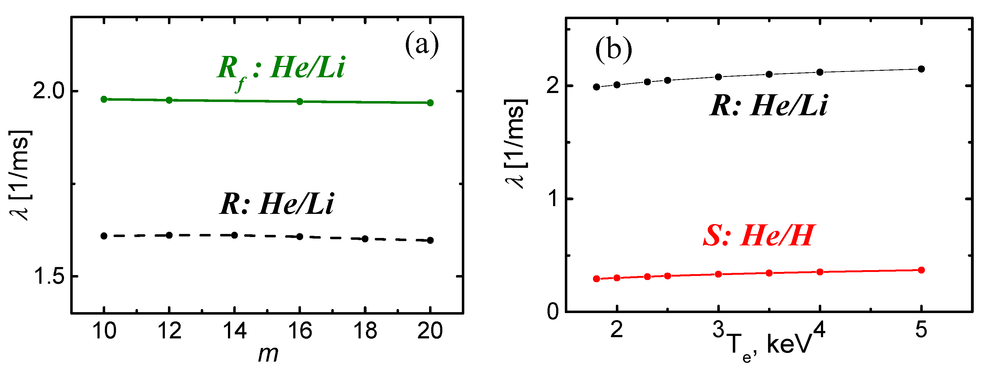
Meanwhile, the simulation results are very weakly dependent on the value of m. For example, Figure 9a shows calculations of the dependence for two types of equilibrium that differ in the total density profile (see Figure 7a). So, λ is weakly sensitive to m, that is, to the radial dimensions of EC’s over a wide range. Similarly, the value λ is weakly sensitive to , while maintaining the shape of the profile . It should be remembered that the ionization rates usually vary slowly near their maxima, depending on the temperature.
4. The Recovery of CS Equilibrium on the Density Profile
As noted above, it is possible to change the formulation of the problem of equilibrium modelling to use the total density profile, , usually known from experiments (or assumed to be given) with the data about ionization rates. Then, the recombination rates could be recovered along with the equilibrium transport rates. Such a formulation can be based on solving Equation (15) after reducing GM to a set of separate REC’s. However, to solve it, it is necessary to have at least approximate data on λ as an input parameter, while the exact value is calculated as Equation (43):
where, initially, knowledge of the functions and is required. Nevertheless, the estimates show that using the total density profile (i.e., the profile taken form the experiment), the approximation can be found by the Equation (44)
Calculations of λ using Equations (43) and (44) for C and Ar are compared in Figure 10. It is seen that all these data can be represented within a good accuracy by two approximate relations. For impurity equilibrium within the K-shell, choosing of He- and H-like ions, we get for both C and Ar, whereas within of He- and Li-like ions we obtain . So, a reasonable approximation to the exact value depends on knowledges of (i) the basis of the equilibrium and (ii) the atomic structure of the most abundant impurity ions. Even rough estimates of the rates of ionization-recombination processes, normalized by an approximate value , provide the necessary input data for modelling using Formula (15) to reduce GM to REC.
Experiments with carbon pellet injection on the LHD stellarator [43] were chosen for modeling, since a large variety of carbon density profiles was observed there. The direct calculation of carbon equilibrium and its quasi-stationary temporal evolution was performed in [17]. These data turn out to be helpful when setting up the proposed recovery model of the profile . So, the recovery model directly uses as input data and reproduces exactly the profiles observed in the LHD. The calculated profiles (and the corresponding charge-exchange recombination rates) are found by an iterative procedure from the calculations of equilibrium. The convergence of iteration procedure in the recovery case is achieved in 8–10 iterations, which is noticeably faster compared to TICS, where it is achieved in only 30–40 iterations.
Figure 11a shows the experimental profiles adopted to discrete case, that is, at s, s, s, s, which are the input data of the model under consideration, except for the profile with carbon accumulation in the center, denoted by the letter A.
As noted in [17], this profile A was modelled using data from the L-mode at s and by adjusting the profile , which determines the cx-recombination rates providing 2D equilibrium. Figure 11b shows the diffusion coefficient profiles calculated by Formula (37). Here we obtain the main feature of equilibrium CS transport in the plasma core, also found in experiments [26], in modelling [17] and revealed by the calculations of the profiles and presented above in Figure 5b: the lower the relative impurity density in the core, the higher . Conversely, the more impurity accumulates in the center, the smaller is required for such an equilibrium.
Figure 11c shows the calculation of the quasi-stationary temporal evolution of the equilibrium function, its successive noticeable flattening and displacement of the sharp edge to the periphery of the plasma column along with the maximum of the density profile . The resulting profiles also change sequentially showing a flattening in the plasma core and a decrease in the density of neutrals at the plasma periphery, where the maximum of shifts. It should be noted that, in general, the obtained novel results are in reasonable agreement with the data of direct modeling of the equilibrium CS transport by the TICS code [17].
5. Conclusions
The impurity CS transport is a typical transport process in plasma, which finds its place in a range of other transport processes. This fundamentally 2D transport is consistently represented by symmetric differential and discrete forms of FPKE. The concept of impurity CS equilibrium transport provides an understanding of the crucial role of atomic processes in the behavior of plasma impurities. The impurity equilibrium observed in experiments together with a large variety of impurity density profiles, both total and partial, in a stationary plasma is essentially a double coronal equilibrium (DCE). DCE is a direct consequence of the symmetric properties of the discrete FPKE (7) and of the conservation law of CS’s moving in the proper phase space.
Nonlinear problems of analysis of 2D CS equilibrium and transport are significantly simplified by reducing the original GM to a whole set of simple schemes (see Figure 4) using the pseudo-state technique together with reduction invariants. The most important of them is the equilibrium constant, λ, which determines the general time scale of the impurity equilibrium in a stationary plasma. It provides crucial information to understand the scale of equilibrium transport rates and confinement time of impurities in hot plasmas.
In particular, the difference of the behavior and transport of impurities in plasma is determined by their ionization-recombination rates values that is, by the dependence , analysis of which is the immediate task. Naturally, the impurity equilibrium and transport in hot plasma depend on the atomic structure of impurity ions that define the equilibrium levels for the most abundant ions as discussed above.
A significant difference of 3–10 times both in the values of D (see Figure 7b) and in the values (see Figure 7 and Figure 8) in various types of CS equilibrium suggests their direct coupling with the observations of impurities in the L-, I -, and H-modes in plasma [25,39]. The estimates made on the basis of CS transport modelling of C and Ar are in good agreement with the known experimental scaling [38] and measurements [39].
The coupling of the profile with the rates of particle transport makes it possible to directly analyze typical profiles and observed in experiments, in particular, for the central accumulation or any other distribution of impurities in the plasma cross-section. It is shown that using REC analysis, data on , ionization-recombination rates and the proposed approximation of λ (see Equation (44)), it is also possible to solve the recovery problem for rate profiles along with equilibrium CS transport analysis. In particular, it is possible to calculate the relative profile of neutral hydrogen, which determines the charge-exchange recombination rate of light and medium impurities.
Thus, the concept of impurity CS transport opens up significant prospects for direct analysis of the rates of ionization-recombination processes in a hot quasi-stationary plasma.
Funding
This research received no external funding.
Institutional Review Board Statement
Not applicable.
Informed Consent Statement
Not applicable.
Data Availability Statement
Not applicable.
Acknowledgments
Author would like to thank V. S. Lisitsa and E. I. Yurchenko for helpful discussions and valuable notes. Author is grateful to V. E. Zhogolev for providing useful software in calculating ionization and recombination rates.
Conflicts of Interest
The authors declare no conflict of interest.
Abbreviations
List of abbreviations used in the paper.
| 1D, 2D, mD | one-dimensional, two-dimensional, multi-dimensional |
| CS, CSs | charge state, charge states |
| FPKE | Fokker-Planck-Kolmogorov Equation |
| DCM | diffusive-convective model |
| GM | grid model |
| CEC | central equilibrium cell |
| CE | coronal equilibrium, the term refers to the 1D balance of ionization/recombination processes, that is, to the charge state distribution of impurity particles |
| DCE | double coronal equilibrium is the 2D balance of impurity charge states |
| EC | equilibrium cell, the 2D reduction scheme shown in Figure 4 |
| REC | reduced equilibrium cell, the 2D reduction scheme shown in Figure 2 |
| CCs | coupled cells, the 2D reduction scheme shown in Figure 4 |
| HL | horizontal line, the 1D reduction scheme shown in Figure 4 |
| VL | vertical line, the 1D reduction scheme shown in Figure 4 |
| SP | separate pair of charge states, the 1D reduction scheme shown in Figure 4 |
| A1, A2, F, H | the types of the total density profiles in Figure 5. |
| TICS | Transport of impurity charge states, numerical transport code described in [17] |
| S-equilibrium is of a 2D one given by the values described by Equation (16) | |
| R- equilibrium is of a 2D one given by the values described by Equation (17) | |
References
- Köchl, F.; Loarte, A.; De La Luna, E.; Parail, V.; Corrigan, G.; Harting, D.; Nunes, I.; Reux, C.; Rimini, F.G.; Polevoi, A.; et al. W transport and accumulation control in the termination phase of JET H-mode discharges and implications for ITER. Plasma Phys. Control. Fusion 2018, 60, 074008. [Google Scholar] [CrossRef]
- Mukai, K.; Nagaoka, K.; Takahashi, H.; Yokoyama, M.; Murakami, S.; Nakano, H.; Ida, K.; Yoshinuma, M.; Seki, R.; LHD Experiment Group; et al. Carbon impurities behavior and its impact on ion thermal confinement in high-ion-temperature deuterium discharges on the Large Helical Device. Plasma Phys. Control. Fusion 2018, 60, 074005. [Google Scholar] [CrossRef]
- Kolmogoroff, A. Über die analytischen Methoden in der Wahrscheinlichkeitsrechnung. Math. Ann. 1931, 104, 415–458. [Google Scholar] [CrossRef]
- Kolmogoroff, A. Zur Theorie der stetigen zufälligen Prozesse. Math. Ann. 1933, 108, 149–160. [Google Scholar] [CrossRef]
- Caughey, T.K. Derivation and Application of the Fokker-Planck Equation to Discrete Nonlinear Dynamic Systems Subjected to White Random Excitation. J. Acoust. Soc. Am. 1963, 35, 1683–1692. [Google Scholar] [CrossRef] [Green Version]
- Dux, R. STRAHL User Manual Technical Report. IPP 10/ 30 IPP Max-Planck-Istitut für Plasmaphysik. 2006. Available online: http://www.ipp.mpg.de/ippcms/de/kontakt/bibliothek/ipp_reports/index.html (accessed on 15 December 2020).
- Bertschinger, G.; Biel, W.; Bitter, M.; Koslowski, H.R.; Krämer-Flecken, A.; Weinheimer, J.; Kunze, H.-J. Behaviour of Ar XVII Spectra in Sawtoothing Discharges at TEXTOR-94. In Proceedings of the 26th EPS Conference on Controlled Fusion Plasma Physics ECA, Maastricht, The Netherlands, 14–18 June 1999; Volume 23J, p. 661, P2.018. Available online: http://epsppd.epfl.ch/Maas/web/pdf/p2018.pdf (accessed on 15 December 2020).
- Sertoli, M.; Angioni, C.; Dux, R.; Neu, R.; Pütterich, T.; Igochine, V.; ASDEX Upgrade Team. Local effects of ECRH on argon transport in L-mode discharges at ASDEX Upgrade. Plasma Phys. Control. Fusion 2011, 53, 035024. [Google Scholar] [CrossRef] [Green Version]
- Stratton, B.; Ramsey, A.; Boody, F.; Bush, C.; Fonck, R.; Groebner, R.; Hulse, R.; Richards, R.; Schivell, J. Spectroscopic study of impurity behaviour in neutral beam heated and ohmically heated TFTR discharges. Nucl. Fusion 1987, 27, 1147–1164. [Google Scholar] [CrossRef]
- Demokan, O.; Waelbroeck, F.; Demokan, N. Iron transport in a confined high-temperature plasma. Nucl. Fusion 1982, 22, 921–934. [Google Scholar] [CrossRef]
- Content, D.; Moos, H.; Perry, M.; Brooks, N.; Mahdavi, M.A.; Petrie, T.; John, H.S.; Schissel, D.; Hulse, R. Impurity profiles for H-mode discharges in DIII-D. Nucl. Fusion 1990, 30, 701–715. [Google Scholar] [CrossRef]
- Stratton, B.; Fonck, R.; Hulse, R.; Ramsey, A.; Timberlake, J.; Efthimion, P.; Fredrickson, E.; Grek, B.; Hill, K.; Johnson, D.; et al. Impurity transport in ohmically heated TFTR plasmas. Nucl. Fusion 1989, 29, 437–447. [Google Scholar] [CrossRef]
- Suckewer, S.; Cavallo, A.; Cohen, S.A.; Daughney, C.C.; Denne, B.; Hinnov, E.; Hosea, J.C.; Hulse, R.A.; Hwang, D.Q.; Schilling, G.; et al. Impurity ion transport studies on the PLT tokamak during neutral-beam injection. Nucl. Fusion 1984, 24, 815–826. [Google Scholar] [CrossRef]
- Asmussen, K.; Fournier, K.; Laming, J.; Neu, R.; Seely, J.; Dux, R.; Engelhardt, W.; Fuchs, J.; ASDEX Upgrade Team. Spectroscopic investigations of tungsten in the EUV region and the determination of its concentration in tokamaks. Nucl. Fusion 1998, 38, 967–986. [Google Scholar] [CrossRef] [Green Version]
- Pütterich, T.; Neu, R.; Dux, R.; Whiteford, A.D.; O’Mullane, M.G.; ASDEX Upgrade Team. Modelling of measured tungsten spectra from ASDEX Upgrade and predictions for ITER. Plasma Phys. Control. Fusion 2008, 50, 085016. [Google Scholar] [CrossRef] [Green Version]
- Hirshman, S.; Sigmar, D. Neoclassical transport of impurities in tokamak plasmas. Nucl. Fusion 1981, 21, 1079–1201. [Google Scholar] [CrossRef]
- Shurygin, V. Impurity charge state transport in tokamak and stellarator plasmas. Nucl. Fusion 2020, 60, 046001. [Google Scholar] [CrossRef]
- Ivanov, V.V.; Kukushkin, A.B.; Lisitsa, V.S. Analytical model of nonstationary kinetics of atom ionization in hot plasmas. Sov. J. Plasma Phys. 1987, 13, 774. [Google Scholar]
- Shurygin, V.A. Anomalous impurity transport: Charge-state diffusion due to atomic processes in tokamak plasmas. Plasma Phys. Control. Fusion 1999, 41, 355–375. [Google Scholar] [CrossRef]
- Shurygin, V.A. Kinetics of impurity charge-state distributions in tokamak plasmas. Plasma Phys. Rep. 2004, 30, 443–472. [Google Scholar] [CrossRef]
- Shurygin, V.A. Analytical approach to impurity transport studies: Charge state dynamics in tokamak plasmas. Phys. Plasmas 2006, 13, 082506. [Google Scholar] [CrossRef]
- Shurygin, V.A. Analytical impurity transport model: Coupling between particle and charge state transports in tokamak plasmas. Phys. Plasmas 2008, 15, 012506. [Google Scholar] [CrossRef]
- TFR Group. Space-resolved vacuum ultra-violet spectroscopy on T.F.R. Tokamak plasmas. Plasma Physics. 1978, 20, 207–223. [Google Scholar] [CrossRef]
- TFR Group. Are heavy impurities in TFR Tokamak plasmas at ionization equilibrium? Plasma Phys. 1980, 22, 851–860. [Google Scholar] [CrossRef]
- Giannella, R.; Lauro-Taroni, L.; Mattioli, M.; Alper, B.; Denne-Hinnov, B.; Magyar, G.; O’Rourke, J.; Pasini, D. Role of current profile in impurity transport in JET L mode discharges. Nucl. Fusion 1994, 34, 1185–1202. [Google Scholar] [CrossRef]
- Dux, R.; Neu, R.; Peeters, A.G.; Pereverzev, G.; Ck, A.M.; Ryter, F.; Stober, J.; ASDEX Upgrade Team. Influence of the heating profile on impurity transport in ASDEX Upgrade. Plasma Phys. Control. Fusion 2003, 45, 1815–1825. [Google Scholar] [CrossRef]
- Braginskii, S.I. Transport Processes in Plasma. In Reviews of Plasma Physics; Leontovich, M.A., Ed.; Consultants Bureau: New York, NY, USA, 1965; Volume 1, pp. 205–311. [Google Scholar]
- Demura, A.V.; Kadomtsev, M.B.; Lisitsa, V.S.; Shurygin, V.A. Tungsten Ions in Plasmas: Statistical Theory of Radiative-Collisional Processes. Atoms 2015, 3, 162–181. [Google Scholar] [CrossRef] [Green Version]
- Wade, M.; Houlberg, W.; Baylor, L.; West, W.; Baker, D. Low-Z impurity transport in DIII-D—Observations and implications. J. Nucl. Mater. 2001, 290, 773–777. [Google Scholar] [CrossRef]
- Kubo, H.; Sakurai, S.; Higashijima, S.; Takenaga, H.; Itami, K.; Konoshima, S.; Nakano, T.; Koide, Y.; Asakura, N.; Shimizu, K.; et al. Radiation enhancement and impurity behavior in JT-60U reversed shear discharges. J. Nucl. Mater. 2003, 313–316, 1197–1201. [Google Scholar] [CrossRef]
- Puiatti, M.E.; Mattioli, M.; Telesca, G.; Valisa, M.; Coffey, I.; Dumortier, P.; Giroud, C.; Ingesson, L.C.; Lawson, K.D.; Contributors to the EFDA-JET Workprogramme; et al. Radiation pattern and impurity transport in argon seeded ELMy H-mode discharges in JET. Plasma Phys. Control. Fusion 2002, 44, 1863–1878. [Google Scholar] [CrossRef] [Green Version]
- Puiatti, M.E.; Valisa, M.; Mattioli, M.; Bolzonella, T.; Bortolon, A.; Coffey, I.; Dux, R.; von Hellermann, M.; Monier-Garbet, P.; Contributors to the EFDA-JET Workprogramme; et al. Simulation of the time behaviour of impurities in JET Ar-seeded discharges and its relation with sawtoothing and RF heating. Plasma Phys. Control. Fusion. 2003, 45, 2011–2024. [Google Scholar] [CrossRef] [Green Version]
- Krupin, V.; Nurgaliev, M.; Klyuchnikov, L.; Nemets, A.; Zemtsov, I.; Dnestrovskij, A.; Sarychev, D.; Lisitsa, V.; Shurygin, V.; Leontiev, D.; et al. Experimental study of tungsten transport properties in T-10 plasma. Nucl. Fusion 2017, 57, 066041. [Google Scholar] [CrossRef]
- Seguin, F.H.; Petrasso, R.; Marmar, E.S. Effects of Internal Disruptions on Impurity Transport in Tokamaks. Phys. Rev. Lett. 1983, 51, 455–458. [Google Scholar] [CrossRef]
- Leung, W.K.; Rowan, W.L.; Wiley, J.C.; Bravenec, R.V.; Gentle, K.W.; Hodge, W.L.; Patterson, D.M.; Phillips, P.E.; Price, T.R.; Richards, B. Interpretation of impurity confinement time measurements in Tokamaks. Plasma Phys. Control. Fusion 1986, 28, 1753–1763. [Google Scholar] [CrossRef]
- Fussmann, G. Analytical modelling of impurity transport in toroidal devices. Nucl. Fusion 1986, 26, 983–1002. [Google Scholar] [CrossRef]
- Mattioli, M.; Puiatti, M.E.; Valisa, M.; Coffey, I.; Dux, R.; Monier-Garbet, P.; Nave, M.F.F.; Ongena, J.; Stamp, M.; Contributors to the EFDA-JET Workprogramme; et al. Simulation of the time behavior of impurities in Jet Ar-seeded discharges and its relation with sawteething. In Proceedings of the 29th EPS Conference on Plasma Physics and Controlled Fusion, Montreux, Switzerland, 17–21 June 2002; ECA Vol. 26B (Geneva: EPS) P2.042 (CD-ROM). Available online: http://epsppd.epfl.ch/Montreux/pdf/P2_042.pdf (accessed on 15 December 2020).
- Mattioli, M.; Giannella, R.; Myrnas, R.; Demichelis, C.; Denne-Hinnov, B.; De Wit, T.D.; Magyar, G. Laser blow-off injected impurity particle confinement times in JET and Tore Supra. Nucl. Fusion 1995, 35, 1115–1124. [Google Scholar] [CrossRef]
- Rice, J.; Reinke, M.; Gao, C.; Howard, N.; Chilenski, M.; Delgado-Aparicio, L.; Granetz, R.; Greenwald, M.; Hubbard, A.; Hughes, J.; et al. Core impurity transport in Alcator C-Mod L-, I- and H-mode plasmas. Nucl. Fusion 2015, 55, 33014. [Google Scholar] [CrossRef] [Green Version]
- Perry, M.; Brooks, N.; Content, D.; Hulse, R.; Mahdavi, M.A.; Moos, H. Impurity transport during the H-mode in DIII-D. Nucl. Fusion 1991, 31, 1859–1875. [Google Scholar] [CrossRef]
- Pasini, D.; Giannella, R.; Taroni, L.L.; Mattioli, M.; Denne-Hinnov, B.; Hawkes, N.; Magyar, G.; Weisen, H. Measurements of impurity transport in JET. Plasma Phys. Control. Fusion 1992, 34, 677–685. [Google Scholar] [CrossRef]
- Krieger, K.; Fussmann, G.; ASDEX Team. Determination of impurity transport coefficients by harmonic analysis. Nucl. Fusion 1990, 30, 2392–2396. [Google Scholar] [CrossRef]
- Ida, K.; Yoshinuma, M.; Osakabe, M.; Nagaoka, K.; Yokoyama, M.; Funaba, H.; Suzuki, C.; Ido, T.; Shimizu, A.; Murakami, I.; et al. Observation of an impurity hole in a plasma with an ion internal transport barrier in the Large Helical Device. Phys. Plasmas 2009, 16, 056111. [Google Scholar] [CrossRef] [Green Version]
Figure 1.
A separate cell of GM with the ratio of rates between nodes.

Figure 2.
Scheme of the REC, which is simply a special case of the EC with .

Figure 3.
Dependence of the limit ratio of densities in the boundary EC under the condition of the defined ionization rate gradient in this cell.
Figure 3.
Dependence of the limit ratio of densities in the boundary EC under the condition of the defined ionization rate gradient in this cell.

Figure 4.
The main schemes of GM reduction by the pseudo-state technique: GM—the initial grid model of impurity distributions, CCs—coupled cells, HL and VL denote horizontal and vertical CS lines, respectively, EC—an equilibrium cell, SP—a separate pair of states.
Figure 4.
The main schemes of GM reduction by the pseudo-state technique: GM—the initial grid model of impurity distributions, CCs—coupled cells, HL and VL denote horizontal and vertical CS lines, respectively, EC—an equilibrium cell, SP—a separate pair of states.

Figure 5.
(a) Typical total impurity density profiles (A1, A2 denote accumulation, F—almost flat, H—hollow) obtained in experiments on the DIII-D [29] (A1 for C), JT-60 [30] (A2 for C) and JET [31,32,37] (A1, A2, F, H for Ar) tokamaks; (b) reduced velocity profiles (dashed) and (dotted) calculated using Formulas (33).

Figure 6.
Dependences of the smallest (in absolute value) non-zero eigenvalue of the matrices , corresponding to the profiles in Figure 5a, on the number of m cells.
Figure 6.
Dependences of the smallest (in absolute value) non-zero eigenvalue of the matrices , corresponding to the profiles in Figure 5a, on the number of m cells.

Figure 7.
The equilibrium of Ar calculated with a recombination (R, Rf curves) and ionization (S curves) equilibrium base: (a) profiles with and without central accumulation; (b) profiles of the diffusivity calculated by Formula (37); (c) S- and R-equilibrium regions determined by the relative profiles of hydrogen neutrals separated by dash-dotted curves showing the limits of the transition region; (d) abrupt change in the equilibrium constant depending on the average impurity charge with a gradual transition between the R and S regions due to changes in the profiles . The dash-dotted curves on (d) show the same limits of the transition region.

Figure 8.
Model calculations of equilibrium constant (a) and confinement time (b) calculated for Ar by Formula (42) with m = 12, various (as denoted), the equilibrium base (for S-equilibrium—full symbols and for R– equilibrium—open symbols), and varying within 1.5–8 keV, corresponding , . The points denoted by JET correspond to the modelling data from JET [17].

Figure 9.
The equilibrium constant of Ar in dependence on (a) the number of cells m; (b) on the central plasma electron temperature .
Figure 9.
The equilibrium constant of Ar in dependence on (a) the number of cells m; (b) on the central plasma electron temperature .

Figure 10.
A comparison of the calculations using the exact Equation (43) and the approximate Equation (44) in the various equilibrium cases of C and Ar. Points shown with open symbols are related to He/Li equilibrium of Ar, while full symbols are of the He/H equilibrium type. Carbon data ( are H-like ions and nucleous) are shown in black triangles.

Figure 11.
The calculated quasi-stationary equilibrium of C in L-mode at s along with modelled central accumulation (curves A) and in H-mode at s, s, s: (a) input total density profiles measured in the experiment [43]; (b) the profiles of diffusion coefficient, calculated according to Formula (37); (c) the equilibrium functions; (d) calculated profiles of the relative density of hydrogen neutrals.

Publisher’s Note: MDPI stays neutral with regard to jurisdictional claims in published maps and institutional affiliations. |
© 2021 by the author. Licensee MDPI, Basel, Switzerland. This article is an open access article distributed under the terms and conditions of the Creative Commons Attribution (CC BY) license (http://creativecommons.org/licenses/by/4.0/).
Share and Cite
MDPI and ACS Style
Shurygin, V.A. Nonlinear Problems of Equilibrium Charge State Transport in Hot Plasmas. Symmetry 2021, 13, 324. https://0-doi-org.brum.beds.ac.uk/10.3390/sym13020324
AMA Style
Shurygin VA. Nonlinear Problems of Equilibrium Charge State Transport in Hot Plasmas. Symmetry. 2021; 13(2):324. https://0-doi-org.brum.beds.ac.uk/10.3390/sym13020324
Chicago/Turabian StyleShurygin, Vladimir A. 2021. "Nonlinear Problems of Equilibrium Charge State Transport in Hot Plasmas" Symmetry 13, no. 2: 324. https://0-doi-org.brum.beds.ac.uk/10.3390/sym13020324
Note that from the first issue of 2016, this journal uses article numbers instead of page numbers. See further details here.