A Review of Many-Body Interactions in Linear and Nonlinear Plasmonic Nanohybrids

Abstract

In this review article, we discuss the many-body interactions in plasmonic nanohybrids made of an ensemble of quantum emitters and metallic nanoparticles. A theory of the linear and nonlinear optical emission intensity was developed by using the many-body quantum mechanical density matrix method. The ensemble of quantum emitters and metallic nanoparticles interact with each other via the dipole-dipole interaction. Surfaces plasmon polaritons are located near to the surface of the metallic nanoparticles. We showed that the nonlinear Kerr intensity enhances due to the weak dipole-dipole coupling limits. On the other hand, in the strong dipole-dipole coupling limit, the single peak in the Kerr intensity splits into two peaks. The splitting of the Kerr spectrum is due to the creation of dressed states in the plasmonic nanohybrids within the strong dipole-dipole interaction. Further, we found that the Kerr nonlinearity is also enhanced due to the interaction between the surface plasmon polaritons and excitons of the quantum emitters. Next, we predicted the spontaneous decay rates are enhanced due to the dipole-dipole coupling. The enhancement of the Kerr intensity due to the surface plasmon polaritons can be used to fabricate nanosensors. The splitting of one peak (ON) two peaks (OFF) can be used to fabricate the nanoswitches for nanotechnology and nanomedical applications.

1. Introduction

Recently there has been considerable interest in studying the nonlinear properties of plasmonic nanohybrids (PNHs) made of metallic nanoparticles and quantum emitters (i.e., quantum dots (QDs)) [1,2,3,4,5,6,7,8,9,10,11,12,13,14,15].

The dipole-dipole interaction in the linear properties of PNHs and photonic crystals has been investigated [10,11,12,13,14]. The Kerr nonlinearity has been studied widely in quantum optics using three-level and four-level atoms [15,16,17,18,19,20,21,22,23,24,25,26,27,28,29,30,31,32,33,34,35,36,37,38,39,40,41,42,43,44,45,46,47,48,49]. For example, giant Kerr nonlinearities in atoms have been studied by using electromagnetically induced transparency. It was shown that the Kerr nonlinear refractive index of a three-level Λ atomic type is greatly enhanced inside an optical ring cavity. On the other hand, the enhancement of the Kerr nonlinearity was also investigated in a four-level atomic system. Experimentally, the enhancement of the Kerr-nonlinear coefficient was also observed in a three-level atomic system such as Rb atom.

Singh [40] studied the nonlinear second harmonic generation in nanohybrids made of a metallic nanoparticle and a QD. Some efforts have also been devoted to studying the Kerr nonlinearity in metallic nanohybrids. Recently, some effort has been devoted to studying the Kerr nonlinearity in PNHs [35,36,37,38,39,40,41,42,43]. For example, Terzis et al. [37] have fabricated optical systems from QD and gold-metallic nanoparticles. Singh experimentally and theoretically [42,43] have studied the nonlinear properties of metallic nanohybrids. The nonlinear effects can also be used for electro-optical device applications such as light modulators, optical switches, optical logic, and optical limiters. The nonlinear research in PNHs can create a revolutionary change in electronic and photonic nontechnology and nanomedicine.

In this review article, we outline a theory we have developed of the linear and nonlinear light emissions for PNHs by using the many-body quantum mechanical density matrix method. A schematic diagram of a nanohybrid containing interacting metallic nanoparticles (MNPs) and quantum emitters (QEs) is shown in Figure 1. In Section 1, we surveyed the literature for the Kerr nonlinearity. In Section 2, a theory of the surface plasmon polaritons due to the photon-plasmon interaction is discussed. In Section 3, the dipole-dipole interaction in the ensemble of QEs and MNPs is explained. In Section 4, a theory for the linear and nonlinear optical absorption intensity using the density matrix method is outlined. In Section 5, we derive the expressions of the spontaneous decay rates due to the dipole-dipole interaction. In Section 6, we show how we derived the expressions of dressed states in the strong exciton-DDI coupling limit. In Section 7, we discuss the simulation we performed on the nonlinear optical absorption intensity. Finally, in the last Section 8, we have summarized the findings of the review article.

2. Surface Plasmon Polaritons

Let us consider a situation where a probe with a frequency ${\omega }_k$ and wave wavevector $k$ is applied to study the PL in the PNH. We know that the surface plasmons are present on the surface of the MNP. The surface plasmons oscillate with a frequency ${\omega }_p$. The probe photons interact with surface plasmons and this interaction creates new quasi-particles called surface plasmon polaritons. Let us calculate the surface plasmon polaritons due to the interaction of photon and surface plasmons interaction as follows.

The Hamiltonian of the surface plasmon and photons, and interactions between them can be written as

$$H_E={\displaystyle {\displaystyle \sum }_k}\hslash {\omega }_k{c}_k^{+}{c}_k+{\displaystyle {\displaystyle \sum }_k}{\omega }_p{B}_k^{+}{B}_k+-{\displaystyle {\displaystyle \sum }_k}{G}_k\left(B_k^{+}{c}_k+B_k{c}_k^{+}\right)$$

(1)

where $c_k^{+}$ and $c_k$ are the photon creation and annihilation operators, respectively. Here $B_k^{+}$ and $B_k$ are the surface plasmon creation and annihilation operators, respectively. The constant $G_k$ is the coupling constant between the photons and plasmons. The first and second terms are for noninteracting photon and plasmon Hamilton. The last term is photon-plasmon interaction Hamiltonian.

Plasmons and photons operators satisfy the following commutation relation.

$$\begin{array}{c}\left[B_k,B_k^{+}\right]={\delta }_{k,k^{\prime }}\\ \left[c_k,c_k^{+}\right]={\delta }_{k,k^{\prime }}\end{array}$$

(2)

Note that in the interaction, the Hamiltonian has a mixture of photon and plasmon operators. We aimed to diagonalize the Hamiltonian. The diagonalization of an interacting Hamiltonian is a standard method in the many-body theory. We defined new quasi-particle creation and annihilation operators $p_{ik}^{+}$ and $p_{ik}^{-}$ with $i=1,2$ We express the plasmon and photon operators in terms of these quasi-particle operators as

$$\begin{array}{c}{B}_k=u_{11}{p}_{1k}+u_{12}{p}_{2k}\\ B_k^{+}=u_{11}^{\ast }{p}_{1k}^{+}+u_{12}^{\ast }{p}_{2k}^{+}\\ c_k=u_{21}{p}_{1k}+u_{22}{p}_{2k}\\ c_k^{+}=u_{21}^{\ast }{p}_{1k}^{+}+u_{22}^{\ast }{p}_{2k}^{+}\end{array}$$

(3)

New quasi-particle operators $p_{ik}^{+}$ and $p_{ik}^{-}$ with i = 1,2 are called surface plasmon polariton operators, which have the combined effect of plasmons and photons.

The Hamiltonian in Equation (1) can be written in the simpler form for diagonalization. It can be expressed as

$$\begin{array}{l}H={\displaystyle \sum _k}{H}_k,\\ H_k=\hslash {\omega }_k{c}_k^{+}{c}_k+{\omega }_p{B}_k^{+}{B}_k-G_k\left(B_k^{+}{c}_k+B_k{c}_k^{+}\right)\end{array}$$

(4)

We aimed to write the $H_k$ in terms of SPP operators $p_{ik}^{+}$ and $p_{ik}^{-}$. Replacing the plasmon and exciton operators in terms of the SPP operators from Equation (3) into Equation (4) and performing extensive mathematical manipulation, we obtained the following expression as

$$H_k=\hslash {\omega }_k^{+}{p}_{1k}^{+}{p}_{1k}+\hslash {\omega }_k^{-}{p}_{2k}^{+}{p}_{2k}$$

(5)

where ${\omega }_k^{+}$ and ${\omega }_k^{-}$ are the energy of SPPs for the upper and lower branches, respectively. Note that coupling between photons and plasmon splits the SPP spectrum into two branches. The SPP spectrum is given by

$${\omega }_k^{\pm }=\frac{1}{2}\left[(ck+{\omega }_p)\pm \sqrt{{(ck-{\omega }_p)}^2+4g_k^2}\right]$$

(6)

where we replaced ${\omega }_k=ck$. Finally, we obtained the expression for the expansion coefficients as

$$\begin{array}{c}{u}_{11}=\sqrt{\frac{g_k^2}{{({\omega }_p-{\omega }_k^{+})}^2+g_k^2,}}\\ u_{21}=\sqrt{\frac{{({\omega }_p-{\omega }_k^{+})}^2}{{({\omega }_p-{\omega }_k^{+})}^2+g_k^2}}\\ u_{22}=\sqrt{\frac{g_k^2}{{({\omega }_p-{\omega }_k^{-})}^2+g_k^2,}}\\ u_{12}=\sqrt{\frac{{({\omega }_p-{\omega }_k^{-})}^2}{{\omega }_p-{\omega }_k^{-}{)}^2+g_k^2}}\end{array}$$

(7)

We then calculated the density of states (DOS) for SPPs. Later in the paper, we discuss how the DOS was used for the calculation of the SPP decay rates. When summation over wavevectors was converted into the integration, we needed to use the idea of the DOS

$$\begin{array}{l}{\displaystyle {\displaystyle {\displaystyle \sum }_k}}=\int D_k({\epsilon }_k)d{\epsilon }_k,\\ D_k({\epsilon }_k)=\frac{\Omega }{3{\pi }^2}{k}^2\frac{dk}{d{\epsilon }_k}\end{array}$$

(8)

where Ω is the volume of the PNH. Here $D_k$ is called the DOS. The expression of the DOS can be expressed in term of the form factor $Z_k$ as

$$\begin{array}{c}D({\epsilon }_k)=D_0({\epsilon }_k)Z_k({\epsilon }_k)\begin{array}{cc},& \end{array}\\ D_0({\epsilon }_k)=\frac{\Omega }{3{\pi }^2}\frac{{\epsilon }_k^2}{{\left(\hslash c\right)}^3,}\\ Z_k({\epsilon }_k)=\left(\hslash c\right)\frac{dk}{d{\epsilon }_k}\end{array}$$

(9)

where $D_0$ is the DOS of photons in free space.

Inserting Equation (6) into Equation (9) and after some mathematical manipulation, the expression of the form factor $Z_k$ could be found as

$$Z_k({\omega }_k^{\pm })=\left(\frac{({\omega }_p-{\omega }_k^{\pm })+{\left|g_k\right|}^2}{{({\omega }_p-{\omega }_k^{\pm })}^2}\right).$$

(10)

We found that the form factor has a very large value when the surface plasmon frequency is the resonance with the SPP frequency, which is an interesting finding.

3. Dipole-Dipole Interactions

When the probe field falls on the PNH, induced dipoles are created in the QEs and MNPs. The dipole of one QE interacts with the dipoles of other QEs. This is called dipole-dipole interaction (DDI). Following reference [10], the DDI Hamiltonian can be written as

$$H_{DDI}^{QE}=\frac{1}{2}{\displaystyle \sum _{i\rangle j}^N}{J}_{ij}{p}_i.p_j$$

(11)

where J_ij is the DDI coupling constant and is found as

$$J_{ij}=\frac{1}{{\in }_b{\in }_0{r}_{ij}^3}$$

(12)

where $p_i$ and $p_j$ are the induced dipole moments in the ith-QE and jth-QE, respectively. Here $r_{ij}$ is the distance between the ith and the jth QEs. In the mean-field approximation [10,44,45,46,47,48,49], the DDI Hamiltonian can be rewritten as

$$H_{DDI}^{QE}={\displaystyle \sum _i^{}}{p}_i{E}_{DDI}^{QE}$$

(13)

where $E_{DDI}^{QE}$ is called the DDI electric field and is written as

$$E_{DDI}^{QE}=\langle \frac{1}{2}{\displaystyle \sum _{j\ne i}^{}}{J}_{ij}{p}_j\rangle .$$

(14)

Here, the DDI field $E_{DDI}^{QE}$ is the average dipole electric field created by all QEs on the ith-QE and that E_DDI has the effect of the long-range DDI (i.e., r⁻³). The average in E_DDI has been evaluated in references [30,31,32,33,34,35,36] by using the method of Lorentz [49], The expression of the DDI field is found as and is written as

$$\begin{array}{l}{E}_{DDI}^{QE}=\frac{{\lambda }_{QD}\langle p_i^{}\rangle }{3\times 4\pi {\in }_0{\in }_b,}\\ \langle p_i^{}\rangle =\frac{P_{QE}}{4\pi R_{QE}^3}\end{array}$$

(15)

where ${\mathsf{\lambda }}_{QD}$ is the DDI constant and $\langle p_i^{}\rangle$ is the average polarization of the ith-QE. Here $P_{QE}$ is the polarization of the QE and $R_{QE}$ is the radius of the quantum emitter.

The probe electric field includes polarizations in the QE and MNP. They are denoted as $P_{QE}$ and $P_{MNP}$. Due to these polarizations, the MNP produces the SPP field $E_{SPP}$ and the QE produces an electric field denoted as $E_{QE}$. Solving Maxwell’s equations in the quasi-static approximation [50,51], one can find the following expressions for polarizations as

$$\begin{array}{l}{P}_{QE}=4\pi {\in }_0{\in }_b{R}_{QE}^3{\zeta }_{QE}\left(E_P^{}+E_{SPP}^{}\right)\\ {\varsigma }_{QE}=\left[\frac{{ϵ}_q-{ϵ}_b}{{ϵ}_q+2{ϵ}_b}\right]\\ P_{MNP}=4\pi {\in }_0{\in }_b{R}_{MNP}^3{\zeta }_{MNP}\left(E_P^{}+E_{QE}^{}\right),\\ {\varsigma }_{MNP}=\left[\frac{{ϵ}_m-{ϵ}_b}{{ϵ}_m+2{ϵ}_b}\right]\end{array}$$

(16)

Here ${ϵ}_m$, ${ϵ}_q$, and ${ϵ}_b$ are the dielectric constant of the MNS, QE and background material, respectively. The electric fields produced by these polarizations were found as

$$\begin{array}{l}{E}_{SPP}=\frac{P_{MNP}}{4\pi {\in }_0{\in }_b{r}_{}^3,}\\ E_{QE}=\frac{P_{QE}}{4\pi {\in }_0{\in }_b{r}_{}^3}\end{array}$$

(17)

Putting Equation (16) into Equation (17), we obtained

$$\begin{array}{l}{E}_{SPP}={\Pi }_{SPP}(E_P^{}+E_{QE}^{})\\ {\Pi }_{SPP}=\frac{R_{MNP}^3{g}_l{\zeta }_{MNP}}{r_{}^3}\\ E_{QE}={\Pi }_{QE}(E_P^{}+E_{SPP}^{})\\ {\Pi }_{QE}=\frac{R_{QE}^3{g}_l{\zeta }_{QE}}{r_{}^3}\end{array}$$

(18)

The constant $g_l$ is called the polarization parameter and it has values $g_l$ = 1 and $g_l$ = −2 for ${\mathit{P}}_{MNP}\parallel \mathit{r}$ and ${\mathit{P}}_{MNP}\perp \mathit{r}$. Note that both electric fields depend on r⁻³. Putting Equation (18) into Equation (14), we obtained the expression of the DDI as

$$\begin{array}{l}{E}_{DDI}^{QE}={\Phi }_{DDI}^{QE}{E}_P^{},\\ {\Phi }_{CDDI}^{QE}=\frac{{\lambda }_{QD}{g}_l{\varsigma }_{MNP}}{3}\\ {\Phi }_{DDI}^{QE}={\Phi }_{CDDI}^{QE}+{\Phi }_{ADDI}^{QE}\\ {\Phi }_{ADDI}^{QE}={\Phi }_{CDDI}^{QE}{\Pi }_{SPP}\end{array}$$

(19)

Similarly, following the above method, we could also calculate the dipole-dipole interaction between MNPs as

$$\begin{array}{l}{E}_{DDI}^{MNP}={\Phi }_{DDI}^{MNP}{E}_P^{}\\ {\Phi }_{CDDI}^{MNP}=\frac{{\lambda }_{MNP}{g}_l{\varsigma }_{MNP}}{3}\\ {\Phi }_{DDI}^{MNP}={\Phi }_{CDDI}^{MNP}+{\Phi }_{ADDI}^{MNP}\\ {\Phi }_{ADDI}^{MNP}={\Phi }_{CDDI}^{MNP}{\Pi }_{QE}\end{array}$$

(20)

Note that the $\Pi$-term and the $\Phi$-term depend on r⁻³. The higher-order terms r⁻⁶ were neglected because they are weak.

4. Linear and Nonlinear Plasmonics and Density Matrix Method

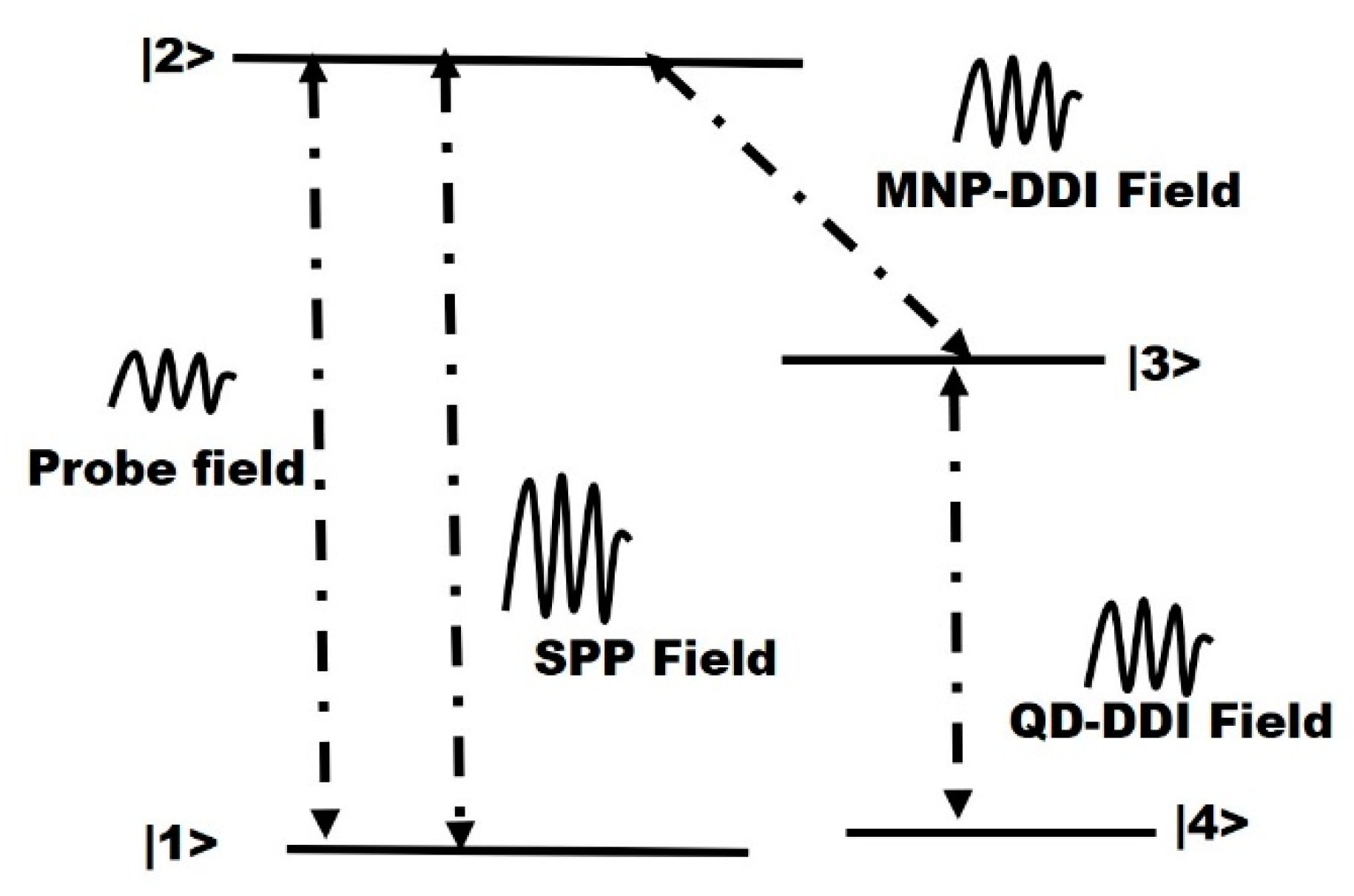
For this section, we calculated the plasmonic Kerr intensity. We considered that QD has four energy levels. They are denoted as |1>, |2>, |3> and |4>. The energy difference between levels |i> and |j> is expressed as ε_ij. To study the Kerr nonlinearity, we applied the probe field between $|\mathbf{1}\rangle$ and $|\mathbf{2}\rangle$. A schematic diagram of the four-level quantum emitter is shown in Figure 2.

Following the method of reference [52,53], the expression of the polarization was found as $P_{QE}$

$$P_{QE}^{}\left({\omega }_p\right)=P_{QE}^{(1)}\left({\omega }_p\right)+P_{QE}^{(2)}\left({\omega }_p,{\omega }_p\right)+P_{QE}^{(3)}\left({\omega }_p,{\omega }_p,{\omega }_p\right)$$

(21)

$$\begin{gathered} P_{QE}^{(1)}\left({\omega }_p\right)={\in }_0{\chi }_{QE}^{(1)}\left({\omega }_p\right)E_p\left({\omega }_p\right) \\ \begin{array}{l}{P}_{QE}^{(2)}\left({\omega }_p,{\omega }_p\right)={\in }_0{\chi }_{QE}^{(2)}\left({\omega }_p,{\omega }_p\right)E_p\left({\omega }_p\right)E_p\left({\omega }_p\right)\\ P_{QE}^{(3)}\left({\omega }_p,{\omega }_p,{\omega }_p\right)={\in }_0{\chi }_{QE}^{(3)}\left({\omega }_p,{\omega }_p,{\omega }_p\right)E_p\left({\omega }_p\right)E_p\left({\omega }_p\right)E_p\left({\omega }_p\right).\end{array} \end{gathered}$$

(22)

Here ${\mathsf{\chi }}_{QE}^{\left(1\right)}$, ${\mathsf{\chi }}_{QE}^{\left(2\right)}$, and ${\mathsf{\chi }}_{QE}^{\left(3\right)}$ are the first, second the third-order expressions of the susceptibility. We know that the first-order susceptibility is responsible for the one-photon phenomena, whereas second-order susceptibility is responsible for the two-photon phenomena. Finally, the third-order susceptibility is responsible for the Kerr nonlinearity.

Fowling the method of references [52,53,54,55], the polarization of the QE can also be expressed in terms of the quantum density matrix operator (ρ) as follows

$$P_{QE}^{}\left({\omega }_p\right)=2{\mu }_{21}\left[{\rho }_{21}^{}\left({\omega }_p\right)+\mathrm{h}.\mathrm{c}.\right]$$

(23)

where ${\mu }_{21}$ is the matrix elements of the dipole moment between transition $\left|1\rangle \leftrightarrow \right|2\rangle$ and ${\rho }_{21}$ is the nonlinear density matrix operator (ρ) between transition $\left|1\rangle \leftrightarrow \right|2\rangle$. Expressing the nonlinear density matrix as follows

$${\rho }_{21}^{}={\rho }_{21}^{(1)}\left({\omega }_p\right)+{\rho }_{21}^{(2)}\left({\omega }_p,{\omega }_p\right)+{\rho }_{21}^{(3)}\left({\omega }_p,{\omega }_p,{\omega }_p\right).$$

(24)

Putting Equation (24) into Equation (23), we obtained

$$P_{QE}^{}\left({\omega }_p\right)=2{\mu }_{21}\left[{\rho }_{21}^{(1)}\left({\omega }_p\right)+{\rho }_{21}^{(2)}\left({\omega }_p,{\omega }_p\right)+{\rho }_{21}^{(3)}\left({\omega }_p,{\omega }_p,{\omega }_p\right)+h.c.\right].$$

(25)

We compared Equations (21) and (25) and we found the relation between the susceptibility and the density matrix elements to be as follows

$$\begin{gathered} {\chi }_{}^{(1)}\left({\omega }_p\right)=\frac{2{\mu }_{21}{\rho }_{21}^{(1)}\left({\omega }_p\right)+hc}{{\in }_0{E}_p\left({\omega }_p\right)} \\ \begin{array}{l}{\chi }_{}^{(2)}\left({\omega }_p,{\omega }_p\right)=\frac{2{\mu }_{21}{\rho }_{21}^{(2)}\left({\omega }_p,{\omega }_p\right)+hc}{{\in }_0{E}_p\left({\omega }_p\right)E_p\left({\omega }_p\right)}\\ {\chi }_{}^{(3)}\left({\omega }_p,{\omega }_p,{\omega }_p\right)=\frac{2{\mu }_{21}{\rho }_{21}^{(3)}\left({\omega }_p,{\omega }_p,{\omega }_p\right)+hc}{{\in }_0{E}_p\left({\omega }_p\right)E_p\left({\omega }_p\right)E_p\left({\omega }_p\right)}\end{array} \end{gathered}$$

(26)

The above expression can be expressed in terms of the Rabi frequency as

$$\begin{gathered} {\chi }_{}^{(1)}\left({\omega }_p\right)=\frac{2{\mu }_{21}^2{\rho }_{21}^{(1)}\left({\omega }_p\right)+hc}{{\in }_0{\hslash }^{}{\Omega }_p^{},} \\ {\chi }_{}^{(2)}\left({\omega }_p,{\omega }_p\right)=\frac{2{\mu }_{21}^3{\rho }_{21}^{(2)}\left({\omega }_p,{\omega }_p\right)+hc}{{\in }_0{\hslash }^2{\Omega }_p^2}, \\ {\chi }_{}^{(3)}\left({\omega }_p,{\omega }_p,{\omega }_p\right)=\frac{2{\mu }_{21}^4{\rho }_{21}^{(3)}\left({\omega }_p,{\omega }_p,{\omega }_p\right)+hc}{{\in }_0{\hslash }^3{\Omega }_p^3} \end{gathered}$$

(27)

Following the method reference [52], the intensity of the fluorescence (light emission intensity) from the QE could be calculated in terms of the susceptibility as follows

$$\begin{gathered} I_{1ph}=\left[\frac{{\omega }_p}{2c{\in }_0\sqrt{{\in }_b}}{\left|{\chi }_{pp}^{(1)}\left({\omega }_p\right)E_p\left({\omega }_p\right)\right|}^2\right] \\ {I}_{2ph}=\left[\frac{{\omega }_p^2}{2c^2{\in }_0\sqrt{{\in }_b}}{\left|{\chi }_{pp}^{(1)}\left({\omega }_p,{\omega }_p\right)E_p\left({\omega }_p\right)E_p\left({\omega }_p\right)\right|}^2\right] \\ {I}_{\ker r}=\left[\frac{{\omega }_p^3}{2c_{}^3{\in }_0\sqrt{{\in }_b}}{\left|{\chi }_{pp}^{(1)}\left({\omega }_p,{\omega }_p,{\omega }_p\right)E_p\left({\omega }_p\right)E_p\left({\omega }_p\right)E_p\left({\omega }_p\right)\right|}^2\right]. \end{gathered}$$

(28)

The expression of the intensity of the fluorescence is given in Equation (28) can be expressed in terms of the density matrix elements by putting Equation (26) into Equation (28) as follows

$$\begin{gathered} I_{1ph}=\frac{4{\omega }_p{\omega }_p{\mu }_{21}^2}{2c{\in }_0{\in }_0^2\sqrt{{\in }_b}}{\left|{\rho }_{21}^{(1)}\left({\omega }_p\right)\right|}^2 \\ \begin{array}{l}{I}_{2ph}=\frac{4{\omega }_p{\omega }_p{\mu }_{21}^2}{2c{\in }_0{\in }_0^2\sqrt{{\in }_b}}{\left|{\rho }_{21}^{(2)}\left({\omega }_p,{\omega }_p\right)\right|}^2\\ I_{\mathrm{kerr}}=\frac{4{\omega }_p{\omega }_p{\mu }_{21}^2}{2c{\in }_0{\in }_0^2\sqrt{{\in }_b}}{\left|{\rho }_{21}^{(3)}\left({\omega }_p,{\omega }_p,{\omega }_p\right)\right|}^2\end{array} \end{gathered}$$

(29)

Note that the susceptibility (Equation (27)) and the fluorescence (Equation (29)) depend on the density matrix elements. Next using the quantum density matrix method, we evaluated the density matrix elements ${\rho }_{21}^{\left(1\right)}$, ${\rho }_{21}^{\left(2\right)},$ and ${\rho }_{21}^{\left(3\right)}$ for the first, second, and third-order in the probe field, respectively.

We know that the probe electric field can be denoted in terms of the Rabi frequency ${\Omega }_P={\mu }_{21}{E}_P/h$ acting between transition $\left|\mathbf{1}\rangle \leftrightarrow \right|\mathbf{2}\rangle$. We consider that the SPP field represented in term of the SPP coupling constant ${\Pi }_{SPP}$ is acting between transition $\left|\mathbf{1}\rangle \leftrightarrow \right|\mathbf{2}\rangle$. Similarly, the DDI-MNP field ${\Phi }_{DDI}^{MNP}$ is acting between transition $\left|\mathbf{2}\rangle \leftrightarrow \right|\mathbf{3}\rangle$ and the DDI-QD field ${\Phi }_{DDI}^{QE}$ is acting between transition $\left|\mathbf{3}\rangle \leftrightarrow \right|\mathbf{4}\rangle$. To make the calculation simple, we considered ${\Phi }_{DDI}={\Phi }_{DDI}^{QE}={\Phi }_{DDI}^{MNP}$. The physics of the problem do not change due to this approximation.

Three electric fields are falling on the QE: $E_T=E_P+E_{DDI}^{MNP}+E_{DDI}^{QE}$. These filed interact with the exciton of the QE. Using the dipole and rotating wave approximation [52,53,54,55], the interaction Hamiltonian between QE was found as

$$H_{in}^{}=\hslash {\Omega }_P{\sigma }_{21}+\hslash {\Omega }_{SPP}^{}{\sigma }_{21}+\hslash {\Omega }_{DDI}^{MNP}{\sigma }_{23}+\hslash {\Omega }_{DDI}^{QE}{\sigma }_{43}+h.c.$$

(30)

where

$$\begin{array}{l}{\Omega }_P=\frac{{\mu }_{21}{E}_P}{\hslash },{\Omega }_{SPP}^{}={\Omega }_P{\Pi }_{SPP},\\ {\Omega }_{DDI}^{MNP}={\Omega }_P{\Phi }_{DDI}^{MNP},{\Omega }_{DDI}^{QE}={\Omega }_P{\Phi }_{DDI}^{QE}\end{array}$$

(31)

Here h.c. stands for the Hermitian conjugate. Here σ_ij = |i><j| is the exciton creation operators for $\left|i\rangle \leftrightarrow \right|j\rangle$. Parameter Ω_p is called the Rabi frequency. The first term in $H_{int}$ is the exciton-probe field interaction. The second term is exciton-SPP field interaction. The third term is exciton-DDI-MNP interaction. The last term is exciton-DDI-QE field interaction.

With the help of Equation (30) and following the method of references [53,54,55] equations of motion for density matrix elements were found as follows

$$\begin{array}{l}\frac{d{\rho }_{11}}{dt}=2{\gamma }_{23}{\rho }_{22}-i{\Omega }_P^{}\left({\rho }_{12}-{\rho }_{21}\right)\\ \frac{d{\rho }_{22}}{dt}=-2{\gamma }_{21}{\rho }_{22}+i{\Omega }_P^{}\left({\rho }_{12}-{\rho }_{21}\right)+i{\Pi }_{SPP}^{}\left({\rho }_{32}-{\rho }_{23}\right)\\ \frac{d{\rho }_{33}}{dt}=2{\gamma }_{31}{\rho }_{22}+i{\Pi }_{SPP}^{}\left({\rho }_{23}-{\rho }_{32}\right)+i{\Phi }_{DDI}^{}\left({\rho }_{43}-{\rho }_{34}\right)*\\ \frac{d{\rho }_{12}}{dt}=-d_{21}{\rho }_{12}-i{\Pi }_{SPP}^{}{\rho }_{13}+i({\rho }_{22}-{\rho }_{11}){\Omega }_P^{}\\ \frac{d{\rho }_{13}}{dt}=-d_{13}{\rho }_{13}-i{\rho }_{12}{\Pi }_{SPP}^{}+i{\rho }_{23}{\Omega }_P^{}-i{\rho }_{14}{\Phi }_{DDI}^{}\\ \frac{d{\rho }_{23}}{dt}=-d_{23}{\rho }_{23}+i({\rho }_{33}-{\rho }_{22}){\Pi }_{SPP}^{}+i{\rho }_{13}{\Omega }_P^{}-i{\rho }_{24}{\Phi }_{DDI}^{}\\ \frac{d{\rho }_{14}}{dt}=-d_{14}{\rho }_{14}-i{\rho }_{13}{\Phi }_{DDI}^{}+i{\rho }_{24}{\Omega }_P^{}\\ \frac{d{\rho }_{24}}{dt}=-d_{24}{\rho }_{24}+i{\rho }_{34}{\Pi }_{SPP}^{}-i{\rho }_{23}{\Phi }_{DDI}^{}+i{\rho }_{13}{\Omega }_P^{}\\ \frac{d{\rho }_{34}}{dt}=-d_{34}{\rho }_{34}+i{\rho }_{24}{\Pi }_{SPP}^{}+i{\Phi }_{DDI}^{}\left({\rho }_{44}-{\rho }_{33}\right)\end{array}$$

(32)

where the parameters appearing in Equation (32) were found as

$$\begin{array}{l}{d}_{21}={\delta }_{21}+i{\gamma }_{21},d_{23}={\delta }_{23}+i{\gamma }_{23},d_{34}={\delta }_{34}+i{\gamma }_{43},\\ d_{41}={\delta }_{41}+i{\gamma }_{41},d_{42}={\delta }_{42}+i{\gamma }_{42},d_{31}={\delta }_{31}+i{\gamma }_{31}\\ {\delta }_{21}={\omega }_{21}-{\omega }_p,{\delta }_{34}={\omega }_{34}-{\omega }_d,{\delta }_{23}={\omega }_{23}-{\omega }_s\\ {\delta }_{42}={\delta }_{23}+{\delta }_{34},{\delta }_{14}={\delta }_{21}-{\delta }_{23}-{\delta }_{34},{\delta }_{13}={\delta }_{21}-{\delta }_{23}\end{array}$$

(33)

Here ${\delta }_{ij}$ is called the field detuning. Physical quantity γ_ij is the exciton decay rates.

We solved Equation (32) in a steady state. We know that density matrix elements satisfy the condition ${\rho }_{11}+{\rho }_{22}+{\rho }_{33}+{\rho }_{44}=0$. We tried to find the analytical expression of the density matrix elements in the steady-state. We considered that initially the ground state is filled and all excited states are empty: ${\rho }_{11}^{\left(0\right)}=1$ and ${\rho }_{22}^{\left(0\right)}+{\rho }_{33}^{\left(0\right)}+{\rho }_{44}^{\left(0\right)}=0$.

In the first order in the probe field, ${\mathsf{\Omega }}_P$, we solved Equation (32) using the above initial condition. After some mathematical manipulations, we obtained the following analytical expression of one-photon density matrix element ${\rho }_{12}^{\left(1\right)}$, as

$${\rho }_{12}^{(1)}=-\frac{i{\Omega }_p\left(d_{13}{d}_{14}-{\Phi }_{DDI}^2\right)}{d_{21}\left(d_{13}{d}_{14}-{\Phi }_{DDI}^2\right)+d_{14}{\Pi }_{SPP}^2}.$$

(34)

The second-order two-photon density matrix element ${\rho }_{12}^{\left(2\right)}$ was calculated in the second order in the probe field, ${\mathsf{\Omega }}_P^2$ by solving Equation (32). After some mathematical manipulations, we obtained the following analytical expression of the element ${\rho }_{12}^{\left(2\right)}$,

$${\rho }_{12}^{(2)}=+\frac{{\rho }_{23}^{(1)}{\Pi }_{SPP}^{}{\Omega }_p^{}{d}_{14}-{\rho }_{24}^{(1)}{\Pi }_{SPP}^{}{\Omega }_p^{}{\Phi }_{DDI}^{}}{d_{21}\left(d_{13}{d}_{14}-d_{21}{\Phi }_{DDI}^2\right)+{\Pi }_{SPP}^2{d}_{14}}+\frac{i\left({\rho }_{22}^{(1)}-{\rho }_{11}^{(1)}\right){\Omega }_p\left(d_{13}{d}_{14}-d_{21}{\Phi }_{DDI}^2\right)}{d_{21}\left(d_{13}{d}_{14}-d_{21}{\Phi }_{DDI}^2\right)+{\Pi }_{SPP}^2{d}_{14}}$$

(35)

$$\begin{array}{l}{\rho }_{24}^{(1)}=-\frac{i{\rho }_{23}^{(1)}{\Phi }_{DDI}^{}{d}_{34}}{d_{24}{d}_{34}+{\Pi }_{SPP}^2}\begin{array}{cc},& \end{array}\\ {\rho }_{24}^{(1)}=-\frac{i{\rho }_{23}^{(1)}{\Phi }_{DDI}^{}{d}_{34}}{d_{24}{d}_{34}+{\Pi }_{SPP}^2}\begin{array}{cc},& \end{array}\\ {\rho }_{22}^{(1)}=\frac{2{\Pi }_{SPP}^{}\mathrm{Im}{\alpha }_{23}^{}}{2{\gamma }_{21}+4{\Pi }_{SPP}^{}\mathrm{Im}{\alpha }_{23}^{}}\\ {\rho }_{23}^{(1)}=\frac{+i{\Pi }_{SPP}^{}\left(d_{24}{d}_{34}+{\Pi }_{SPP}^2\right)({\rho }_{33}^{(1)}-{\rho }_{22}^{(1)})}{d_{23}\left(d_{24}{d}_{34}+{\Pi }_{SPP}^2\right)+{\Phi }_{DDI}^2{d}_{34}}\begin{array}{cc},& \end{array}\\ {\alpha }_{23}=\frac{+i{\Pi }_{SPP}^{}\left(d_{24}{d}_{34}+{\Pi }_{SPP}^2\right)}{d_{23}\left(d_{24}{d}_{34}+{\Pi }_{SPP}^2\right)+{\Phi }_{DDI}^2{d}_{34}}\end{array}$$

(36)

The third order Kerr density matrix element ${\rho }_{12}^{\left(3\right)}$ was calculated in the third order in the probe field ${\mathrm{E}}_P^3$ and ${\mathrm{E}}_{SPP}^3$ by solving Equation (32). After some mathematical manipulations, we obtained the following analytical expression of the element ${\rho }_{12}^{\left(3\right)}$ as

$${\rho }_{12}^{(3)}=\frac{{\rho }_{23}^{(2)}{\Omega }_p^{}{\Pi }_{SPP}^{}{d}_{14}+i{\rho }_{24}^{(2)}{\Omega }_p^{}{\Phi }_{DDI}^{}{\Lambda }_{SPP}^{}}{d_{21}\left(d_{13}{d}_{14}-d_{21}{\Phi }_{DDI}^2\right)+{\Pi }_{SPP}^2{d}_{14}}+\frac{i({\rho }_{22}^{(2)}-{\rho }_{11}^{(2)}){\Omega }_p\left(d_{13}{d}_{14}-d_{21}{\Pi }_{SPP}^2\right)}{d_{21}\left(d_{13}{d}_{14}-d_{21}{\Phi }_{DDI}^2\right)+{\Pi }_{SPP}^2{d}_{14}}$$

(37)

$$\begin{array}{l}{\rho }_{13}^{(1)}=-\left(\frac{d_{14}{\Phi }_{DDI}^{}{\Omega }_p}{d_{21}\left(d_{13}{d}_{14}-{\Pi }_{SPP}^2\right)+d_{14}{\Phi }_{DDI}^2}\right)\begin{array}{cc},& \end{array}\\ {\rho }_{24}^{(2)}=-\frac{i{\rho }_{23}^{(2)}{\Pi }_{SPP}^{}{d}_{34}}{d_{24}{d}_{34}+{\Phi }_{DDI}^2}\\ {\rho }_{23}^{(2)}=\frac{\left(i{\rho }_{33}^{(2)}{\Phi }_{DDI}^{}-i{\rho }_{22}^{(2)}{\Phi }_{DDI}^{}+i{\rho }_{13}^{(1)}{\Omega }_P\right)\left(d_{24}{d}_{34}+{\Phi }_{DDI}^2\right)}{\left(d_{24}{d}_{34}+{\Phi }_{DDI}^2\right)+{\Pi }_{SPP}^2{d}_{34}}\begin{array}{cc},& \end{array}\\ {\rho }_{22}^{(2)}=\frac{{\Omega }_p^{}\mathrm{Im}\left({\rho }_{12}^{(1)}\right)}{{\gamma }_{21}}\end{array}$$

(38)

Note that the ${\rho }_{12}^{\left(1\right)}$, ${\rho }_{12}^{\left(2\right)}$, and ${\rho }_{12}^{\left(3\right)}$ depend on the SPP and DDI couplings.

We then calculated the linear fluorescence intensity due to the emission of one photon. Inserting Equation (34) into Equation (29) we obtained linear fluorescence intensity as

$$I_{1ph}=\frac{4{\omega }_p{\omega }_p{\mu }_{21}^2}{2c{\in }_0{\in }_0^2\sqrt{{\in }_b}}{\left|\frac{i{\Omega }_p\left(d_{13}{d}_{14}-{\Phi }_{DDI}^2\right)}{d_{21}\left(d_{13}{d}_{14}-{\Phi }_{DDI}^2\right)+d_{14}{\Pi }_{SPP}^2}\right|}^2.$$

(39)

Similarly, we calculated the nonlinear fluorescence intensity due to the emission of two photons. Inserting Equation (35) into Equation (29) we obtained the two-photon fluorescence intensity as

$$\begin{gathered} I_{2ph}=\frac{4{\omega }_p{\omega }_p{\mu }_{21}^2}{2c{\in }_0{\in }_0^2\sqrt{{\in }_b}}{\left|{\rho }_A^{(2)}\left({\omega }_p,{\omega }_p\right)+{\rho }_B^{(2)}\left({\omega }_p,{\omega }_p\right)\right|}^2 \\ {\rho }_A^{(2)}\left({\omega }_p,{\omega }_p\right)=+\frac{{\rho }_{23}^{(1)}{\Pi }_{SPP}^{}{\Omega }_p^{}{d}_{14}-{\rho }_{24}^{(1)}{\Pi }_{SPP}^{}{\Omega }_p^{}{\Phi }_{DDI}^{}}{d_{21}\left(d_{13}{d}_{14}-d_{21}{\Phi }_{DDI}^2\right)+{\Pi }_{SPP}^2{d}_{14}} \\ {\rho }_B^{(2)}\left({\omega }_p,{\omega }_p\right)=\frac{i\left({\rho }_{22}^{(1)}-{\rho }_{11}^{(1)}\right){\Omega }_p\left(d_{13}{d}_{14}-d_{21}{\Phi }_{DDI}^2\right)}{d_{21}\left(d_{13}{d}_{14}-d_{21}{\Phi }_{DDI}^2\right)+{\Pi }_{SPP}^2{d}_{14}}. \end{gathered}$$

(40)

Finally, we evaluated the nonlinear fluorescence intensity due to the emission of three photons. Inserting Equation (37) into Equation (29), we obtained three-photon fluorescence intensity (i.e., Kerr intensity) as

$$\begin{gathered} I_{\mathrm{kerr}}=I_0{\left|\frac{\left({\rho }_A^{(3)}+{\rho }_A^{(3)}\right)}{d_{21}\left(d_{13}{d}_{14}-d_{21}{\Lambda }_{DDI}^2\right)+{\Lambda }_{SPP}^2{d}_{14}}\right|}^2 \\ \begin{array}{l}{\rho }_A^{(3)}={\rho }_{23}^{(2)}{\Omega }_p^{}{\Pi }_{SPP}^{}{d}_{14}+i{\rho }_{24}^{(2)}{\Omega }_p^{}{\Phi }_{DDI}^{}{\Pi }_{SPP}^{},\\ I_0=\frac{4{\omega }_{21}{\omega }_{21}{\mu }_{21}^2}{2c{\in }_0{\in }_0^2\sqrt{{\in }_b}}\end{array} \\ {\rho }_B^{(3)}=i({\rho }_{22}^{(2)}-{\rho }_{11}^{(2)}){\Omega }_P\left(d_{13}{d}_{14}-d_{21}{\Pi }_{SPP}^2\right). \end{gathered}$$

(41)

We found that the one-photon, two-photon, and three-photon fluorescence intensity depends on the SPP coupling and DDI couplings.

5. Exciton Decay Rates Due to Dipole-Dipole Interaction

The radiative decay rates ${\mathsf{\gamma }}_{ij}$ appear in Equations (27)–(35). The radiative decay rate ${\mathsf{\gamma }}_{21}$ is due to the spontaneous emission of exciton transition from $|2\rangle$ to $|1\rangle$. The decay rate ${\mathsf{\gamma }}_{23}$ is due to the exciton decay from $|2\rangle$ to $|3\rangle$ because of the exciton-DDI-MNP interaction. Similarly, the decay rate ${\mathsf{\gamma }}_{34}$ is also due to the exciton decay from $|3\rangle$ to $|4\rangle$ because of the exciton-DDI-QD interaction.

The SPP dispersion relation ${\omega }_k^{\pm }$ was evaluated in Equation (6) for the upper (+) and lower (−) SPP spectrum. The lower mode of the SPP is responsible for the enhancement of the SPP field. Hence, we consider the lower branch for the decay calculation. The spectrum of the lower branch was denoted as ${\omega }_k^s={\omega }_k^{-}$. Henceforth, we take out superscript (−) for all terms.

The exciton interaction Hamiltonian with the probe, SPP, and DDI fields can be written in the dipole and rotating wave approximation as

$$H_{\mathrm{int}}=H_0+H_{ex-PP}^{}+H_{ex-SPP}^{}+H_{ex-DDI}^{MNP}+H_{ex-DDI}^{QD}$$

(42)

where the first term is the Hamiltonian for the noninteracting excitons and SPPs. The second term is due to the spontaneous emission coupling term due to the exciton-probe field interaction. The third term is due to the exciton-SPP field interaction. Finally, the fourth and fifth terms are due to the exciton-DDI field interaction. Their expressions were found as

$$\begin{array}{l}{H}_0={\displaystyle \sum _{i=1,3}^{}}\hslash {\omega }_{i1}{\sigma }_{i1}+{\displaystyle {\displaystyle \sum }_k}\hslash {\omega }_k^s{p}_k^{†}{p}_k^{}\\ H_{ex-PP}={\displaystyle {\displaystyle \sum }_k}{V}_{PP}^{}\left(p_k^{}{\sigma }_{21}^{†}+p_k^{†}{\sigma }_{21}^{}\right)\begin{array}{cc},& \end{array}\\ H_{ex-SPP}^{}={\displaystyle {\displaystyle \sum }_k}{V}_{SPP}^{}\left(p_k^{}{\sigma }_{21}^{†}+p_k^{†}{\sigma }_{21}^{}\right)\\ H_{ex-DDI}^{MNP}={\displaystyle {\displaystyle \sum }_k}{V}_{DDI}^{MNP}\left(p_k^{}{\sigma }_{23}^{†}+p_k^{†}{\sigma }_{23}^{}\right)\begin{array}{cc},& \end{array}\\ H_{ex-DDI}^{QE}={\displaystyle {\displaystyle \sum _k}}{V}_{DDI}^{QE}\left(p_k^{}{\sigma }_{34}^{†}+p_k^{†}{\sigma }_{34}^{}\right)\end{array}$$

(43)

where σ_ij = |i><j| is the exciton creation operator for transition $\left|i\rangle \leftrightarrow \right|j\rangle$ where i and j stand for 1, 2, 3, and 4. Meanwhile, the operators $p_{nm,k_z}^{†}{p}_{nm,k_z}^{}$ are the photon creation and annihilation operators, respectively. The coupling constant appearing in Equation (43) was found as

$$\begin{array}{l}{V}_{PP}=i{\left(\frac{{\mu }_{21}^2\hslash {\omega }_k^s}{2{\in }_0{\in }_b{V}_{QE}}\right)}^{1/2}\\ V_{SPP}^{}=i{\left(\frac{{\mu }_{21}^2\hslash {\omega }_k^s}{2{\in }_0{\in }_b{V}_{QE}}\right)}^{1/2}\left[{\Pi }_{SPP}^{}\right]\\ V_{DDI}^{MNP}=i{\left(\frac{{\mu }_{23}^2\hslash {\omega }_k^s}{2{\in }_0{\in }_b{V}_{QD}}\right)}^{1/2}\left[{\Phi }_{DDI}^{MNP}\right]\begin{array}{cc},& \end{array}\\ V_{DDI}^{QE}=i{\left(\frac{{\mu }_{34}^2\hslash {\omega }_k^s}{2{\in }_0{\in }_b{V}_{QE}}\right)}^{1/2}\left[{\Pi }_{DDI}^{QE}\right]\end{array}$$

(44)

where $V_{QE}$ is the volume of the QE.

The Golden rule method of the quantum mechanical perturbation theory was used to calculate the decay rates. It is written as

$${\Gamma }_{ij}=2\pi \hslash {\displaystyle {\displaystyle \sum _k}}{\displaystyle \int d{\omega }_k^s}{D}_k\left({\omega }_k^s\right){\left|V_{\mathrm{int}}^{}\left({\omega }_k^s\right)\right|}^2\delta \left({\omega }_k^s-{\epsilon }_{ij}\right)$$

(45)

where V_int is the interaction term given in Equation (44) and D_k is the DOS which has been calculated in Equation (8).

Putting Equations (44) and (8) into Equation (45) and doing extensive mathematical manipulations, we obtained the decay rates for exciton as

$${\Gamma }_P^{}={\gamma }_0{Z}_k\left({\omega }_{21}\right)={\gamma }_0\left(\frac{({\omega }_p-{\omega }_{21})+{\left|g_k\right|}^2}{{({\omega }_p-{\omega }_{21})}^2}\right)\begin{array}{cc},& \end{array}{\gamma }_0=\left(\frac{{\hslash }^3{\mu }_{21}^2{\omega }_{21}^3}{\pi {\in }_0{\in }_b{\hslash }^4{c}^3}\right)$$

(46)

$$\begin{array}{l}{\Gamma }_{SPP}^{}={\gamma }_0{\left|{\Pi }_{SPP}^{}\right|}^2{Z}_k\left({\omega }_{21}\right)\\ {\Gamma }_{DDI}^{MNP}={\gamma }_0\left|{\Lambda }_{DDI}^{MNP}\right|Z_k\left({\omega }_{23}\right)\\ {\Gamma }_{DDI}^{QD}={\gamma }_0{\left|{\Lambda }_{DDI}^{QD}\right|}^2{Z}_k\left({\omega }_{34}\right)\end{array}$$

(47)

Here γ₀ is the radiative decay rate when QD is in the vacuum. Please note the following relationship ${\gamma }_{21}={\Gamma }_P^{}+{\Gamma }_{SPP}^{}$, ${\gamma }_{23}={\Gamma }_{DDI}^{MNP}$ and ${\gamma }_{34}={\Gamma }_{DDI}^{QE}$. Note that the radiative and nonradiative decay rates can have large values when exciton energies ε₁₂, ε_23, and ε₃₄ are close to ${\epsilon }_{nm}$. This is an interesting finding of the paper.

6. Dressed States: Exciton-DDI Coupling

We show in the next section that in the strong coupling between the exciton and DDI polaritons, the single peak in the Kerr absorption splits into two peaks. This phenomenon can be easily explained by the physics of the dressed state. We calculated the energies and eigenfunctions for exciton-DDI polariton Hamiltonian in the strong coupling. Note that the DDI field is acting between states |2> and |3>. For simplicity we denoted |3> and |2> as |a> and |b>, respectively. Here |a> and |b> are the ground state and the excited state of the exciton.

The polariton energy of the kth mode was denoted as ${\epsilon }_k={\epsilon }_d$ and it was considered that the energy of the DDI polariton is very close to exciton energy i.e., ${\epsilon }_k~{\epsilon }_{ba}$. This means that only one mode of the polariton was acting with an exciton and we denoted ${\epsilon }_k={\epsilon }_{DDI}$. The interaction Hamiltonian between exciton and the DDI polaritons was written as in the dipole and rotating wave approximation can be written as

$$H_T={\epsilon }_a{\sigma }_{aa}+{\epsilon }_b{\sigma }_{bb}+{\epsilon }_d{p}_k^{+}{p}_k-\hslash {\Omega }_{DDI}\left({\sigma }_{ba}^{+}{p}_k+{\sigma }_{ba}^{-}{p}_k^{+}\right).$$

(48)

Here $p_k^{+}$ and $p_k$ are the DDI polariton creation and annihilation operators, respectively. Here $\left|a><a\right|$ and $\left|b><b\right|$ are called the number operators for states |a> and |b>, respectively. The first two terms are the noninteracting Hamilton for the exciton and kth mode DDI polariton. The last term is the exciton-polariton interaction Hamiltonian. The constant ${\Omega }_{DDI}$ is called the Rabi frequency for the DDI field.

We then calculated the eigenvalues and eigenfunctions of the total Hamiltonian as

$$H_T|{\phi }_k\rangle ={\epsilon }_T|{\phi }_k\rangle$$

(49)

where are ${\epsilon }_T$ and $|{\phi }_k\rangle$ are the eigenvalue and eigenket of the total Hamiltonian $H_{int}$. We considered two states which have the same number of particles, i.e., $n_k$. Therefore, we choose $|a, n_k\rangle$ and $|b, n_k-1\rangle$ states. The first has $n_k$ polaritons and zero excitons and the second has one exciton and $\left(n_k-1\right)$ polaritons. Note that both states form $|a, n_k\rangle$ and $|b, n_k-1\rangle$ form an orthonormal set and they satisfy the orthonormal conditions as follows

$$\langle a,n_k|a,n_k\rangle =1,\hspace{1em}\langle b,n_k-1|b,n_k-1\rangle =1,\hspace{1em}\langle a,n_k|b,n_k-1\rangle =0.$$

(50)

The eigenket $|{\phi }_k\rangle$ can be expressed as a linear combination of the orthonormal set $|a, n_k\rangle$ and $|b, n_k-1\rangle$ as

$$|{\phi }_k\rangle ={\alpha }_a|a,n_k\rangle +{\alpha }_b|b,n_k-1\rangle$$

(51)

where ${\alpha }_a$ and ${\alpha }_b$ are expansion constants. Inserting Equation (51) into Equation (49) and using Equation (50), we obtained the following equations after some mathematical manipulations as

$$\left(\begin{array}{cc}\left\{{\epsilon }_T-({\epsilon }_a+{\epsilon }_{n_k})\right\}& \left(\hslash {\Omega }_a\sqrt{n_k}\right)\\ -\left(\hslash {\Omega }_a\sqrt{n_k}\right){\alpha }_a& \left\{{\epsilon }_T-({\epsilon }_b+{\epsilon }_{n_k-1})\right\}\end{array}\right)\left(\begin{array}{c}{\alpha }_a\\ {\alpha }_b\end{array}\right)=0.$$

(52)

The determinant of the above equation gives the eigenvalues of energy ${\epsilon }_T$ as

$$\left|\begin{array}{cc}\left\{{\epsilon }_T-({\epsilon }_a+{\epsilon }_{n_k})\right\}& \left(\hslash {\Omega }_a\sqrt{n_k}\right)\\ -\left(\hslash {\Omega }_a\sqrt{n_k}\right){\alpha }_a& \left\{{\epsilon }_T-({\epsilon }_b+{\epsilon }_{n_k-1})\right\}\end{array}\right|=0.$$

(53)

The above expression reduces to the following equation as

$${\epsilon }_T^{\pm }=\left(\frac{{\epsilon }_b+{\epsilon }_{n_k-1}+{\epsilon }_b+{\epsilon }_{n_k}}{2}\right)\pm \frac{1}{2}\sqrt{{\left({\epsilon }_d-{\epsilon }_{ba}\right)}^2+4n_k{\hslash }^2{\left|{\Omega }_{ddi}\right|}^2}.$$

(54)

The ${\epsilon }_T^{+}$ and ${\epsilon }_T^{-}$ are eigenvalues for eigenkets $|{\phi }_T^{+}\rangle$ and $|{\phi }_T^{-}\rangle$ and they are called dressed states. Putting, ${\epsilon }_{n_k}=n_k{\epsilon }_d$ and ${\epsilon }_{ba}={\epsilon }_b-{\epsilon }_a$ into the above expression, we obtained

$${\epsilon }_T^{\pm }=\left(\frac{{\epsilon }_{ba}}{2}+\left\{n_k-\frac{1}{2}\right\}{\epsilon }_d\right)\pm \frac{1}{2}\sqrt{{\left({\epsilon }_d-{\epsilon }_{ba}\right)}^2+4n_k{\hslash }^2{\left|{\Omega }_{ddi}\right|}^2}.$$

(55)

We then calculated the eigenkets $|{\phi }_T^{+}\rangle$ and $|{\phi }_T^{-}\rangle$ from Equation (48) for eigenvalues ${\epsilon }_T^{+}$ and ${\epsilon }_T^{-}$. The expansion coefficients ${\alpha }_a^{\pm }$ and ${\alpha }_b^{\pm }$ are provided in Equations (56) and (57). Using orthonormalization properties given in Equation (50) and after some mathematical manipulation, we obtained

$${\alpha }_b^{\pm }={\left(\frac{{\left\{{\epsilon }_T^{\pm }-({\epsilon }_a+{\epsilon }_{n_k})\right\}}^2}{{\left\{{\epsilon }_T^{\pm }-({\epsilon }_a+{\epsilon }_{n_k})\right\}}^2+{\left(\hslash {\Omega }_{ddi}\sqrt{n_k}\right)}^2}\right)}^2$$

(56)

$${\left({\alpha }_a^{\pm }\right)}^2={\left(\frac{\hslash {\Omega }_{ddi}\sqrt{n_k}}{{\left\{{\epsilon }_T^{\pm }-({\epsilon }_a+{\epsilon }_{n_k})\right\}}^2+{\left(\hslash {\Omega }_{ddi}\sqrt{n_k}\right)}^2}\right)}^{1/2}.$$

(57)

In most of the experiments, only one polariton was required to excite transition from ground state |a〉 to the excited state |b〉. Therefore, we added $n_k=1$ in the above equations. For this case, we obtained the following expression for the eigenvalues

$${\epsilon }_T^{\pm }=\left(\frac{{\delta }_{ba}}{2}+{\epsilon }_{ba}\right)\pm \frac{1}{2}\sqrt{{\left({\delta }_{ba}\right)}^2+4{\hslash }^2{\left|{\Omega }_{ddi}\right|}^2}$$

(58)

Here ${\delta }_{ba}={\epsilon }_{ba}-{\epsilon }_d$ is called the detuning parameter in quantum optics. When the DDI polariton energy is in resonance with the exciton transition energy (i.e., ${\delta }_{ba}={\epsilon }_{ba}-{\epsilon }_d=0$), the above expression reduces to a simple form

$${\epsilon }_T^{\pm }={\epsilon }_{ab}\pm {\hslash }^2{\left|{\Omega }_{ddi}\right|}^2.$$

(59)

We found that when the polariton energy is in resonance with the exciton energy, the excited state splits into two dressed states $|{\phi }_T^{+}\rangle$ and $|{\phi }_T^{-}\rangle$. The energy difference between the two dressed state was proportional to the DDI coupling ${\Omega }_{ddi}={\Omega }_P{\Phi }_{ddi}$.

7. Results and Discussion

In this section, we discuss the numerical simulations performed on the SPP dispersion relation, DOS of SPPs, and Kerr absorption intensity. The effect of the SPP and DDI couplings on the Kerr absorption intensity are also investigated. In our numerical simulations, we measured all physical qualities related to energy (frequency) are measured with respect to the decay rate γ₂. Some of the examples for the energy (frequency) physical quantities are Rabi frequency (Ω_P), exciton frequencies, probe detuning, and decay rates. In our numerical simulations, we used γ₂₃/γ₂₁ = γ₃₄/γ₂₁=1 and Ω_P /γ₂₁ = 1. The probe detuning (δ_p) and DDI detuning (δ_d) were measured with respect to the decay rate γ₂₁.

We first calculated the dispersion relation for the SPPs and the density of states for the SPPs. Here the dispersion relation means the relation between the energy and wavevector of polaritons. The dispersion relation is calculated in Equation (6) and the DOS is calculated in Equation (9). The results are presented in Figure 3a,b. The normalized SPP energy (${\omega }_k^{\pm }/{\omega }_p$) is plotted in Figure 3a as a function of a normalized wave vector $(k/k_p$). One can see that the SPP dispersion relation has a bandgap. The upper band does not participate in the enhancements of the Kerr intensity because its properties are similar to photons. On the other hand, the lower band plays an important role in plasmonics. The behavior of this band is a mixture of plasmons and photons (i.e., SPPs). These materials can be called the polaritonic bandgap materials, since they have a polaritonic bandgap in their band structure. They are similar to photonic bandgap materials that have a bandgap in their photonic dispersion relations.

The results for DOS are plotted in Figure 3b as a function of the normalized energy (${\omega }_k^{\pm }/{\omega }_p$). We found that the DOS has large values near the band edges. This means that a large number of SPPs are located near the band edges. When a QE lies near the MNP, excitons of the QE interact with the SPPs of MNPs. However, if the energy of the excitons lies near the band edges, there will be huge exciton-SPP coupling since there are the huge number of polaritons are located near the band edges.

Next, we studied the effect of the SPP field on the Kerr absorption intensity ($I_{kerr}/I_0)$. The results are plotted in Figure 4a as a function of normalized detuning (${\delta }_p/{\mathsf{\gamma }}_{21}={\delta }_{21}/{\mathsf{\gamma }}_{21}$) for different values of the SPP coupling (${\Pi }_{SPP}$). For Figure 4a, we have considered that DDI coupling is absent. The solid, dash, and dash-dotted lines were plotted for the detuning parameter ${\Pi }_{SPP}=0.1$, ${\Pi }_{SPP}=0.7$, and ${\Pi }_{SPP}=1.5,$ respectively. Note that the SPP coupling is unitless. Other parameters are taken as ${\Phi }_{DDI}=0.0$. Her the DDI coupling is also unitless. Note that at zero detuning (i.e., δ_p/${\mathsf{\gamma }}_{21}$ = 0), the Kerr intensity has a peak. The zero detuning means that the probe field frequency is in resonance with the exciton frequency ${\omega }_{21}$ (i.e., ${\omega }_p={\omega }_{21})$.

We found in Figure 4a that as the SPP coupling increases, the Kerr intensity also increases. See the dotted and dash-dotted lines in the figure. This means that there is a large enhancement in the Kerr intensity due to the presence of SPPs. The enhancement occurred because the SPP coupling appears in the numerator of the Kerr intensity expression. See Equation (41). Further, we predicted that the enhancement has smaller values when the probe field is not in resonance with the exciton energy.

We also plotted a three-dimensional figure for the Kerr intensity ($I_{kerr}/I_0)$ as a function of the SPP coupling (${\Pi }_{SPP})$ and the probe detuning $\left({\delta }_p/{\mathsf{\gamma }}_{21}\right)$. The results are shown in Figure 4b. Note that as the SPP coupling increases, the Kerr effect also increases. There is a huge enhancement in the Kerr intensity due to the nonreality of the system.

The enhancement in both Figure 4a,b in the Kerr absorption intensity can be explained as follows. When the SPP field (i.e., MNS) is absent (i.e., ${\Pi }_{SPP}=0$ ), the Kerr intensity is due to the contribution from three probe photons. However, the Kerr intensity has an extra contribution due to the SSP coupling. The extra contribution to the Kerr intensity is due to the three polaritons produced by the SPP field. The SPP contributions to the Kerr intensity are many times larger than the probe photons. In summary, we can say that the present finding can be used to fabricate nanosensor devices for nanotechnology and nanomedical applications by measuring the enhancement of the Kerr intensity.

Next, we investigated the effect of the DDI coupling (${\Phi }_{DDI})$ on the Kerr intensity ($I_{kerr}/I_0)$. The results are plotted in Figure 5a as a function of the probe detuning $\left({\delta }_p/{\mathsf{\gamma }}_{21}\right)$. The solid, dash, and dash-dotted lines were plotted for the detuning parameter ${\Phi }_{DDI}=0.1$, ${\Phi }_{DDI}=0.5$, and ${\Phi }_{DDI}=2.0$ respectively. The SPP coupling parameter was taken as ${\Pi }_{SPP}=0.1$. The SPP and DDI coupling parameters were unitless. One can see from the figure that for the DDI coupling ${\Phi }_{DDI}=0.5$, the Kerr intensity was enhanced. When the DDI coupling was further increased to ${\Phi }_{DDI}=2.0$, the Kerr intensity decreased, and one peak split into two peaks.

To make the effect of the DDI coupling on the Kerr intensity clearer, we plotted a three-dimensional figure of the Ker nonlinearity in Figure 5b. Note that when the DDI coupling is in the weak coupling limit, the Kerr intensity increases with the DDI coupling. It reaches a maximum value at a certain value of the DDI (i.e., ${\Phi }_{DDI}=0.4$). When the DDI coupling increases further, the peak of the Kerr intensity splits into two-peaks. In summary, we can say that when ${\Phi }_{DDI}<1$.

The Kerr intensity has one peak. On the other hand, when ${\Phi }_{DDI}>1$, the Kerr intensity splits from one peak to two peaks. The condition ${\Phi }_{DDI}<1$ is called the weak coupling limit, whereas the condition ${\Phi }_{DDI}>1$ is called the strong coupling limit. This is an interesting finding of the paper.

We then defined the weak and strong DDI coupling limits. In the literature, the weak coupling limit is defined when the Rabi frequency of the DDI electric field (${\Omega }_{DDI}$) is smaller than the decay rate (i.e., ${\Omega }_{DDI}<{\gamma }_{21}$). Here the DDI Rabi frequency is defined as ${\Omega }_{DDI}={\Phi }_{DDI}{\Omega }_P$. In this case, the DDI coupling ${\Phi }_{DDI}$ is in the weak coupling limit. On the other hand, the strong coupling limits are defined when the DDI Rabi frequency is larger than the decay rate $({\Omega }_{DDI}<{\gamma }_{21})$. In this case, the DDI coupling is in the strong coupling limit. The above definitions are the approximate definition and are not applied in all problems. Note that in Figure 5b, the DDI coupling approximately satisfies the weak and strong coupling limit criteria for the enhancement and the splitting of the peak.

The splitting from one peak to two peaks due to the strong DDI coupling limit is explained by using the physics of dressed states, as discussed in Section 5. In the absence of the DDI coupling, the Kerr intensity is due to the three photons emission from the transition $\left|2\rangle \leftrightarrow \right|1\rangle$. On the other hand, in the strong DDI coupling limit the excited state $\left|2\rangle \leftrightarrow \right|3\rangle$ splits into two dressed states $\left|2_{-}\rangle \leftrightarrow \right|3\rangle$ and $\left|2_{+}\rangle \leftrightarrow \right|3\rangle$. Therefore, the Kerr intensity emissions have two peaks due to transitions $\left|2_{-}\rangle \leftrightarrow \right|1\rangle$ and $\left|2_{+}\rangle \leftrightarrow \right|1\rangle$. We have also found that the distance between the peaks increases as the DDI coupling increases. This is because the energy splitting is directly related to the DDI coupling. See Equation (59) for further details. In summary, we can say that the splitting of one peak (ON) into two peaks (OFF) can be used to fabricate nanoswitching devices for nanotechnology and nanomedical applications.

Finally, we provide comments on the giant nonlinearity found due to the Kerr effect in the present work. We have shown that there is a huge (giant) enhancement in Kerr nonlinearity due to the presence of SPPs. We have also found the due to the weak DDI coupling, there is also an enhancement in the Kerr nonlinearity. The giant Kerr nonlinearity found in plasmonic nanohybrids is of great importance in the context of quantum information theory and its applications. In particular, the photon/phonon blockade can appear in systems involving high Kerr-type nonlinearities [56,57]. Moreover, such systems can be applied in the maximally entangled state’s generation [58] and as the source of quantum steering [59]. Quite recently, the model involving Kerr nonlinearities was considered in the context of the PT-symmetry breaking [60]. The present study can also be used for optical pumping [61] and photon transparency [62].

8. Conclusions

A theory of the Kerr nonlinear tensity was developed by using the many-body quantum mechanical density matrix method for plasmonic nanohybrids. We showed that the Kerr intensity enhances in the weak dipole-dipole coupling limits. On the other hand, in the strong dipole-dipole coupling limit, the single peak in the Kerr intensity splits into two peaks. Further, we found that the Kerr nonlinearity is also enhanced due to the SPP coupling. Next, we determined the spontaneous decay rates are enhanced due to the dipole-dipole coupling. The enhancement of the Kerr intensity due to the surface plasmon polaritons can be used to fabricate nanosensors. The splitting of one peak (ON) two peaks (OFF) can be used to fabricate the nanoswitches for nanotechnology and nanomedical applications.

References

- Artuso, R.D.; Bryant, G.W. Strongly coupled quantum dot-metal nanoparticle systems: Exciton-induced transparency, discontinuous response, and suppression as driven quantum oscillator effects. Phys. Rev. B 2010, 82, 195419. [Google Scholar] [CrossRef]
- Yannopapas, V.; Paspalakis, E. Giant enhancement of dipole-forbidden transitions via lattices of plasmonic nanoparticles. J. Mod. Opt. 2015, 62, 1435–1441. [Google Scholar] [CrossRef]
- Tame, M.S.; McEnery, K.R.; Özdemir, Ş.K.; Lee, J.; Maier, S.A.; Kim, M.S. Quantum plasmonics. Nat. Phys. 2013, 9, 329–340. [Google Scholar] [CrossRef] [Green Version]
- Törmä, P.; Barnes, W.L. Strong coupling between surface plasmon polaritons and emitters: A review. Rep. Prog. Phys. 2015, 78, 013901. [Google Scholar] [CrossRef] [PubMed]
- Achermann, M. Exciton−Plasmon Interactions in Metal−Semiconductor Nanostructures. J. Phys. Chem. Lett. 2010, 1, 2837. [Google Scholar] [CrossRef]
- Singh, M.R.; Guo, J.; Fanizza, E.; Dubey, M. Anomalous photoluminescence quenching in metallic nanohybrids. J. Phys. Chem. C 2019, 123, 10013–10020. [Google Scholar] [CrossRef]
- Balakrishnan, S.; Najiminaini, M.; Singh, M.R.; Carson, J.J.L. A study of angle dependent surface plasmon polaritons in nano-hole array structures. J. Appl. Phys. 2016, 120, 034302. [Google Scholar] [CrossRef]
- Antón, M.A.; Carreño, F.; Melle, S.; Calderon, O.G.; Granado, E.C.; Singh, M.R. Optical pumping of a single hole spin in ap-doped quantum dot coupled to a metallic nanoparticle. Phys. Rev. B 2013, 87, 195303. [Google Scholar] [CrossRef] [Green Version]
- Racknor, C.; Singh, M.R.; Zhang, Y.; Birch, D.J.S.; Chen, Y. Energy transfer between a biological labelling dye and gold nanorods. Methods Appl. Fluoresc. 2013, 2, 015002. [Google Scholar] [CrossRef] [Green Version]
- Singh, M.R.; Black, K. Anomalous dipole-dipole interaction between ensemble of quantum emitters in metallic nanoparticle hybrids. J. Phys. Chem. C 2018, 122, 26584–26591. [Google Scholar] [CrossRef]
- Yudson, V.I.; Singh, M.R. Lattice-gas model for electron-hole coupling in disordered media. Phys. Rev. B 1998, 58, 16202. [Google Scholar] [CrossRef]
- Singh, M.R.; Guo, J.; Chen, J. A Theoretical Study of Fluorescence Spectroscopy of Quantum Emitters Coupled with Plasmonic Dimer and Trimer. J. Phys. Chem. C 2019, 123, 17483–17490. [Google Scholar] [CrossRef]
- Singh, M.R. The effect of the dipole–dipole interaction in electromagnetically induced transparency in polaritonic band gap materials. J. Mod. Opt. 2007, 54, 1739–1757. [Google Scholar] [CrossRef]
- Singh, M.R. Dipole-Dipole Interaction in Photonic-Band-Gap Materials Doped with Nanoparticles. Phys. Rev. A 2007, 75, 043809. [Google Scholar] [CrossRef]
- Schmidt, H.; Imamoglu, A. Giant Kerr nonlinearities obtained by electromagnetically induced transparency. Opt. Lett. 1996, 21, 1936–1938. [Google Scholar] [CrossRef] [PubMed]
- Wang, H.; Goorskey, D.; Xiao, M. Enhanced Kerr Nonlinearity via Atomic Coherence in a Three-Level Atomic System. Phys. Rev. Lett. 2001, 87, 073601. [Google Scholar] [CrossRef] [PubMed] [Green Version]
- Yan, X.-A.; Wang, L.-Q.; Yin, B.-Y.; Jiang, W.-J.; Zheng, H.-B.; Song, J.-P.; Zhang, Y.-P. Effect of spontaneously generated coherence on Kerr nonlinearity in a four-level atomic system. Phys. Lett. A 2008, 372, 6456–6460. [Google Scholar] [CrossRef]
- Khoa, D.X.; Van Doai, L.; Son, D.H.; Bang, N.H. Enhancement of self-Kerr nonlinearity via electromagnetically induced transparency in a five-level cascade system: An analytical approach. J. Opt. Soc. Am. B 2014, 31, 1330–1334. [Google Scholar] [CrossRef]
- Ren, J.; Chen, H.; Gu, Y.; Zhao, D.; Zhou, H.; Zhang, J.; Gong, Q. Plasmon-enhanced Kerr nonlinearity via subwavelength-confined anisotropic Purcell factors. Nanotechnology 2016, 27, 425205. [Google Scholar] [CrossRef] [PubMed]
- Doai, L.V.; Khoa, D.X.; Bang, N.H. EIT enhanced self-Kerr nonlinearity in the three-level lambda system under Doppler broadening. Phys. Scr. 2015, 90, 45502. [Google Scholar] [CrossRef]
- Sheng, J.; Yang, X.; Wu, H.; Xiao, M. Modified self-Kerr-nonlinearity in a four-level N-type atomic system. Phys. Rev. A 2011, 84, 053820. [Google Scholar] [CrossRef]
- Singh, M.R. Two-photon absorption in photonic nanowires made from photonic crystals. J. Opt. Soc. Am. B 2009, 26, 1801–1807. [Google Scholar] [CrossRef]
- Berland, K.; So, P.; Gratton, E. Two-photon fluorescence correlation spectroscopy: Method and application to the intracellular environment. Biophys. J. 1995, 68, 694–701. [Google Scholar] [CrossRef] [Green Version]
- Jung, J.-M.; Yoo, H.-W.; Stellacci, F.; Jung, H.-T. Two-Photon Excited Fluorescence Enhancement for Ultrasensitive DNA Detection on Large-Area Gold Nanopatterns. Adv. Mater. 2010, 22, 2542–2546. [Google Scholar] [CrossRef]
- Li, X.; Kao, F.-J.; Chuang, C.-C.; He, S. Enhancing fluorescence of quantum dots by silica-coated gold nanorods under one- and two-photon excitation. Opt. Express 2010, 18, 11335–11346. [Google Scholar] [CrossRef] [PubMed]
- Gao, D.; Agayan, R.R.; Xu, H.; Philbert, M.A.; Kopelman, R. Nanoparticles for Two-Photon Photodynamic Therapy in Living Cells. Nano Lett. 2006, 6, 2383–2386. [Google Scholar] [CrossRef] [Green Version]
- Yuan, H.; Khoury, C.G.; Hwang, H.; Wilson, C.M.; A Grant, G.; Vo-Dinh, T. Gold nanostars: Surfactant-free synthesis, 3D modelling, and two-photon photoluminescence imaging. Nanotechnology 2012, 23, 075102. [Google Scholar] [CrossRef] [Green Version]
- Albota, M.; Beljonne, D.; Brédas, J.L.; Ehrlich, J.E.; Fu, J.Y.; Heikal, A.A.; Hess, S.E.; Kogej, T.; Levin, M.D.; Marder, S.R.; et al. Design of Organic Molecules with Large Two-Photon Absorption Cross Sections. Science 1998, 281, 1653–1656. [Google Scholar] [CrossRef] [Green Version]
- Singh, M.R.; Persaud, P.D. Dipole−dipole Interaction in two-photon spectroscopy of metallic nanohybrids. J. Phys. Chem. C. 2020, 124, 6311–6320. [Google Scholar] [CrossRef]
- Singh, M.R.; Persaud, P.D.; Yastrebov, S. A study of two-photon florescence in metallic nanoshells. Nanotechnology 2020, 31, 265203. [Google Scholar] [CrossRef] [PubMed]
- Fejer, M.M. Nonlinear Optical Frequency Conversion. Phys. Today 1994, 47, 25–32. [Google Scholar] [CrossRef]
- Cerullo, G.; De Silvestri, S. Ultrafast optical parametric amplifiers. Rev. Sci. Instrum. 2003, 74, 1–18. [Google Scholar] [CrossRef]
- Sugioka, K. Progress in ultrafast laser processing and future prospects. Nanophotonics 2017, 6, 393–413. [Google Scholar] [CrossRef] [Green Version]
- Potma, E.O.; De Boeij, W.P.; Wiersma, D.A. Nonlinear coherent four-wave mixing in optical microscopy. J. Opt. Soc. Am. B 2000, 17, 1678–1684. [Google Scholar] [CrossRef] [Green Version]
- Yannopapas, V.; Paspalakis, E. Optical properties of hybrid spherical nanoclusters containing quantum emitters and metallic nanoparticles. Phys. Rev. B 2018, 97, 205433. [Google Scholar] [CrossRef]
- Tohari, M.M.; Lyras, A.; AlSalhi, M.S. Giant Self-Kerr Nonlinearity in the Metal Nanoparticles-Graphene Nanodisks-Quantum Dots Hybrid Systems Under Low-Intensity Light Irradiance. Nanomaterials 2018, 8, 521. [Google Scholar] [CrossRef] [PubMed] [Green Version]
- Terzis, A.; Kosionis, S.; Boviatsis, J.; Paspalakis, E. Nonlinear optical susceptibilities of semiconductor quantum dot—Metal nanoparticle hybrids. J. Mod. Opt. 2015, 63, 451–461. [Google Scholar] [CrossRef]
- Liu, Q.; He, X.; Zhao, X.; Ren, F.; Xiao, X.; Jiang, C.; Zhou, X.; Lu, L.; Zhou, H.; Qian, S.; et al. Enhancement of third-order nonlinearity in Ag-nanoparticles-contained chalcohalide glasses. J. Nanoparticle Res. 2011, 13, 3693–3697. [Google Scholar] [CrossRef]
- Kelly, K.L.; Coronado, E.; Zhao, L.L.; Schatz, G.C. The Optical Properties of Metal Nanoparticles: The Influence of Size, Shape, and Dielectric Environment. J. Phys. Chem. B 2003, 107, 668–677. [Google Scholar] [CrossRef]
- Singh, M.R. Enhancement of the second-harmonic generation in a quantum dot–metallic nanoparticle hybrid system. Nanotechnolgy 2013, 24, 125701. [Google Scholar] [CrossRef] [PubMed]
- Cox, J.D.; Singh, M.R.; Von Bilderling, C.; Bragas, A.V. A Nonlinear Switching Mechanism in Quantum Dot and Metallic Nanoparticle Hybrid Systems. Adv. Opt. Mater. 2013, 1, 460–467. [Google Scholar] [CrossRef]
- Singh, M.R. Theory of all-optical switching based on the Kerr nonlinearity in metallic nanohybrids. Phys. Rev. A 2020, 102, 013708. [Google Scholar] [CrossRef]
- Singh, M.R.; Yastrebov, S. Switching and Sensing Using Kerr Nonlinearity in Quantum Dots Doped in Metallic Nanoshells. J. Phys. Chem. C 2020, 124, 12065–12074. [Google Scholar] [CrossRef]
- Mazenko, G.F. Quantum Statisitcal Mechanics; John Wiley and Sons Inc.: New York, NY, USA, 2000; Section 5.8. [Google Scholar]
- Kittel, C. Introduction to Solid State Physics, 6th ed.; John Wiley and Sons Inc.: New York, NY, USA, 1996; Chapter 13. [Google Scholar]
- Ali Omar, M. Elementary Solid State Physics; Addison-Wesley: New York, NY, USA, 1993; Section 8.11. [Google Scholar]
- Gerstein, J.L.; Smith, F.W. The Physics and Chemistry of Materials; John Wiley and Sons Inc.: New York, NY, USA, 2001; Chapter 15. [Google Scholar]
- Eyring, H. Statistical Mechanics and Dynamics; Dover: New York, NY, USA, 1952. [Google Scholar]
- Lorentz, H. The Theory of Electrons; Dover: New York, NY, USA, 1952. [Google Scholar]
- Novotny, L.; Hecht, B. Principle of Nano-Optics; Cambridge University Press: Cambridge, UK, 2006. [Google Scholar]
- Sarid, D.; Challener, W.A. Modern Introduction to Surface Plasmons: Theory, Mathematica Modeling, and Applications; Cambridge University Press: Cambridge, UK, 2010. [Google Scholar]
- Hanamura, E.; Kawabe, Y.; Yamanaka, A. Quantum Nonlinear Optics; Springer: Tokyo, Japan, 2007. [Google Scholar]
- Boyd, R.W. Nonlinear Optics, 3rd ed.; Academic Press: New York, NY, USA, 2008. [Google Scholar]
- Singh, M.R. Electronic, Photonic, Polaritonic and Plasmonic Materials; Wiley Custom: Toronto, ON, Canada, 2014. [Google Scholar]
- Scully, M.O.; Zubairy, M.S. Quantum Optics; Cambridge University Press: London, UK, 1997. [Google Scholar]
- Leoński, W.; Tanaś, R. Possibility of producing the one-photon state in a kicked cavity with a nonlinear Kerr medium. Phys. Rev. A 1994, 49, R20–R23. [Google Scholar] [CrossRef]
- Imamoḡlu, A.; Schmidt, H.; Woods, G.; Deutsch, M. Strongly Interacting Photons in a Nonlinear Cavity. Phys. Rev. Lett. 1997, 79, 1467–1470. [Google Scholar] [CrossRef]
- Leoński, W.; Miranowicz, A. Kerr nonlinear coupler and entanglement. J. Opt. B Quantum Semiclass. Opt. 2004, 6, S37. [Google Scholar] [CrossRef] [Green Version]
- Kalaga, J.K.; Leoński, W.; Szczȩśniak, R. Quantum steering and entanglement in three-mode triangle Bose–Hubbard system. Quantum Inf. Process. 2017, 16, 265. [Google Scholar] [CrossRef]
- Peřina, J., Jr.; Lukš, A.; Kalaga, J.K.; Leoński, W.; Miranowicz, A. Non-classical light at exceptional points of a quantum PT-symmetric two-mode system. Phys. Rev. A 2019, 100, 53820. [Google Scholar] [CrossRef] [Green Version]
- Antón, M.; Carreño, F.; Melle, O.S.; Calderón, E.; Cabrera-Granado, M. Singh Transparency in semiconductor-metal nanoparticle hybrid system. Phys. Rev. B 2013, 87, 195303. [Google Scholar] [CrossRef] [Green Version]
- Singh, M.R. Photon transparency in metallic photonic crystals doped with an ensemble of nanoparticles. Phys. Rev. A 2009, 79, 013826. [Google Scholar] [CrossRef]
Figure 1.
Schematic diagram of a nanohybrid which consists of a noninteracting metallic nanoparticles (MNPs) and interacting quantum emitters (QEs).
Figure 2.
A schematic diagram of a four-level quantum dots (QDs) is plotted. Energy levels are denoted as |1>, |2>, |3> and |4>. The probe field and SPP field are applied in the transition . The DDI-MNP and DDI-QD fields are acting in the transitions and , respectively.
Figure 3.
(a) (left): The band structure of the SPPs is plotted as a function of the normalized energy and wavevectors. (b) (right): The DOS of the SPPs is plotted as a function of the normalized energy.
Figure 4.
(a) (left): The Kerr absorption intensity ( is plotted as a function of the normalized probe detuning . The solid, dash, and dash-dotted lines are plotted for , , and , respectively. (b) (right): The Kerr absorption intensity ( is plotted as a function of the SPP coupling ΠSPP (normalized unit) and the probe detuning (normalized unit).
Figure 5.
(a) (left): The Kerr intensity ( plotted as a function of the probe detuning . The solid, dash and dash-dotted lines are plotted for the detuning parameter , , and respectively. (b) (right): The Kerr intensity ( plotted as a function of the probe detuning and the DDI coupling .
Publisher’s Note: MDPI stays neutral with regard to jurisdictional claims in published maps and institutional affiliations. |
© 2021 by the author. Licensee MDPI, Basel, Switzerland. This article is an open access article distributed under the terms and conditions of the Creative Commons Attribution (CC BY) license (http://creativecommons.org/licenses/by/4.0/).
Share and Cite
MDPI and ACS Style
Singh, M.R. A Review of Many-Body Interactions in Linear and Nonlinear Plasmonic Nanohybrids. Symmetry 2021, 13, 445. https://0-doi-org.brum.beds.ac.uk/10.3390/sym13030445
AMA Style
Singh MR. A Review of Many-Body Interactions in Linear and Nonlinear Plasmonic Nanohybrids. Symmetry. 2021; 13(3):445. https://0-doi-org.brum.beds.ac.uk/10.3390/sym13030445
Chicago/Turabian StyleSingh, Mahi R. 2021. "A Review of Many-Body Interactions in Linear and Nonlinear Plasmonic Nanohybrids" Symmetry 13, no. 3: 445. https://0-doi-org.brum.beds.ac.uk/10.3390/sym13030445
Note that from the first issue of 2016, this journal uses article numbers instead of page numbers. See further details here.