
Effective Rotor Fault Diagnosis Model Using Multilayer Signal Analysis and Hybrid Genetic Binary Chicken Swarm Optimization


Department of Electrical Engineering, Chung Yuan Christian University, No. 200, Zhongbei Road, Zhongli District, Taoyuan City 320, Taiwan
*
Author to whom correspondence should be addressed.
Symmetry 2021, 13(3), 487; https://0-doi-org.brum.beds.ac.uk/10.3390/sym13030487
Submission received: 12 February 2021
/
Revised: 2 March 2021
/
Accepted: 9 March 2021
/
Published: 16 March 2021
(This article belongs to the Special Issue Simulation and Modelling in Natural Sciences, Economics, Biomedicine and Engineering II)
Abstract
:This article proposes an effective rotor fault diagnosis model of an induction motor (IM) based on local mean decomposition (LMD) and wavelet packet decomposition (WPD)-based multilayer signal analysis and hybrid genetic binary chicken swarm optimization (HGBCSO) for feature selection. Based on the multilayer signal analysis, this technique can reduce the dimension of raw data, extract potential features, and remove background noise. To compare the validity of the proposed HGBCSO method, three well-known evolutionary algorithms are adopted, including binary-particle swarm optimization (BPSO), binary-bat algorithm (BBA), and binary-chicken swarm optimization (BCSO). In addition, the robustness of three classifiers including the decision tree (DT), support vector machine (SVM), and naive Bayes (NB) was compared to select the best model to detect the rotor bar fault. The results showed that the proposed HGBCSO algorithm can obtain better global exploration ability and a lower number of selected features than other evolutionary algorithms that are adopted in this research. In conclusion, the proposed model can reduce the dimension of raw data and achieve high robustness.
1. Introduction
Rotating machines are among the most significant devices in the industry field. Many rotating machines that break down usually cause an unexpected operation. In the worst case, rotating machine failures cause tremendous economic losses or serious casualties. One of the most critical components of rotating machines is the rotor. Rotor bar failure will cause speed and torque fluctuations and lead to shaft vibration, which leads to the premature failure of other motor components [1]. Thus, early detection for the rotor fault can also help prevent other types of fault, like bearing or eccentricity [2]. Considering the reliability and performance of rotating machines, the authors have conducted in-depth research and proposed some fault diagnosis models, which have achieved good results. For example, Brkovic et al. proposed a simpler, faster, and accurate bearing early fault detection and diagnosis technique based on scatter matrices and quadratic classifiers [3]. Gligorijevic et al. presented a new online condition monitoring technique for early fault detection and diagnosis to prevent the unexpected faulty operation of bearings [4]. Van et al. used various bearing fault diagnosis models by improved non-local-mean de-noising and empirical mode decomposition (EMD) feature extraction and two-stage feature selection [5]. Helmi et al. proposed a model for the fault detection and diagnosis of rolling bearings structure based on time domain and frequency domain features of the extraction of the vibration signal and the adaptive neuro-fuzzy interface system network. Their experimental results enabled the detection of faults in rotating machines and the categories of faults with high accuracy [6].
The most widely used techniques for fault detection are motor current signature analysis (MCSA), vibration signal analysis, and acoustic sound signals analysis [7]. All these techniques for fault detection have advantages and weaknesses. The MCSA technique has the advantages of being noninvasive and easy to implement. However, under certain conditions, its application is not sensitive enough because it has a low signal-to-noise ratio. Its other disadvantages include its spectral leakage and low-frequency resolution. The downside of acoustic sound signal analysis is its sensitivity to external noise. The technique of acoustic emission, which measures the acoustic signals in the ultrasonic range providing a high signal-to-noise ratio, has the disadvantage of requiring more complex implementation [8]. Vibration signal analysis has high potential for fault detection as it is easy to measure and can extract favorable fault features. Because vibration signals contain noisy, non-linear, and non-stationary components, some time-frequency analysis such as short-time Fourier transform (STFT), Wigner–Ville distribution (WVD), wavelet transform (WT), Hilbert-Huang transform (HHT) and empirical mode decomposition (EMD), have become the most effective techniques in recent years. However, the above techniques have their own limitations. For example, STFT is limited to a fixed length of the window [9]. WVD is limited by cross-terms interference for the non-stationary signals [10]. WT is suitable for non-stationary signal processing with high resolution to solve the above problems from STFT and WVD [11,12]. However, when analyzing the practical signal, the pre-defined wavelet-based parameters may not completely guarantee efficiency for practical signal processing and analysis, which makes WT non-adaptive [13]. For vibration signals, the self-adaptive signal analysis may be more efficient [14]. As proposed by Huang et al. [15], EMD adaptively decomposes the non-stationary signals into a set of intrinsic mode functions (IMFs). However, EMD is limited by end effects and mode mixing [16,17,18].
Similar principles with EMD, local mean decomposition (LMD) is a self-adaptive time-frequency domain analysis method first proposed by J. S. Smith in 2005 that has good results for the analysis of EEG signals [19]. The LMD decomposes the signal into a set of product functions (PFs), each of which is the product of an envelope signal and a frequency modulated signal. LMD has many potential properties. First, LMD directly obtains instantaneous amplitude and instantaneous frequency without Hilbert transform (HT) [19]. Second, LMD solves the over-/undershoot problem by using the moving averaging method to compute the local mean [20]. Third, the end effects and mode mixing problem already alleviate or are not obvious in LMD [21,22]. Fourth, compared with EMD, LMD decomposes the signal into fewer components, and that each component contains more useful information [22]. However, in the practical fault diagnosis of rotating machines, the vibration signals acquisitioned from sensors always contain huge noise, which causes LMD to decompose additional and redundant frequency components. To solve this problem, the wavelets de-noising technique such as wavelet packet decomposition (WPD) has obtained good results to implement signal denoising [23,24,25]. To extract the useful features from the vibration signal and remove noise, the multilayer signal analysis method is applied in three steps as follows. First, the LMD decomposes the original signal into a set of PFs. Then, the PF selection method is used to select effective components. Then, WPD is used to further extract feature information and denoise. Finally, the statistical features are extracted from these components.
In order to build a good model prediction, strongly relevant features should be selected and irrelevant, redundant, or noisy features should be eliminated [26]. The feature selection method is applied to remove uncorrelated features to obtain the optimal feature subset. In recent decades, evolutionary algorithms such as particle swarm optimization (PSO), bat algorithm (BA), and chicken swarm optimization (CSO) have been used for feature selection. However, each algorithm has its own limitations. For example, BA cannot balance between its exploration and exploitation capability [27]. Both BA and PSO are suffer from premature convergence and easily fall into the local optimal when computing high-dimension problems [27,28]. CSO was a new evolutionary algorithm proposed by Meng et al. in 2014 [29], which has good ability in terms convergence rate and convergence accuracy. Nevertheless, like PSO and BA, the basic CSO has the same limitation of premature convergence and easy to fall into local optima [30]. Therefore, the researchers have proposed many improved CSO, which achieved good results [30,31,32]. In this research, combining with basic CSO and genetic algorithm (GA), it is called hybrid genetic binary chicken swarm optimization (HGBCSO). Based on GA, the crossover operation is an effective tool to improve the global search ability and population diversity [33]. Moreover, two positions updating strategies are adopted to improve global exploration abilities. By using these improvements, HGBCSO can balance exploration and exploitation and avoid premature convergence.
The solutions present in evolutionary algorithms for feature selection are binary strings in binary search space [34]. In this research, the above algorithms are applied for feature selection as binary-PSO (BPSO) [35], binary-BA (BBA) [36,37], and binary-CSO (BCSO) [38,39].
The last task of the proposed model is to classify the optimal feature subset. In recent years, neural networks and machine learning algorithms are widely using in the field of machinery fault diagnosis [40,41]. Compared with neural networks, machine learning algorithms have the advantages of higher classification performance [42,43,44,45]. Therefore, three machine learning algorithms, including decision tree (DT), support vector machine (SVM), and naive Bayes (NB) are applied and compared robustness in this research. The DT-based diagnosis models are natural, which may not need the knowledge for researchers and can be easily applied to diagnosis models. However, the DT classifier is suffering from overfitting and low generalization performance which would reduce the diagnosis performance. The NB-based diagnosis models are easy to achieve fault diagnosis with multiple states. However, because of the low ability of data fitting, it is difficult to represent the complicated function relationship. The SVM is a widely used machine learning method for fault diagnosis. The SVM-based diagnosis models can easily obtain the global optimal solution and further obtain the high diagnostic accuracy based on the objective solution of convex quadratic optimization [46]. In conclusion, this article proposes a rotor bar fault diagnosis model, which uses a multilayer signal analysis to extract fault features, and uses HGBCSO for feature selection.
In this article, the main points can be summarized as three points:
- Proposing a multilayer signal analysis method combining two signal processing methods (LMD and WPD) and PF selection. This technique can reduce the dimension of original data, descend background noise, and extract potential features.
- Proposing a feature selection method using the combination with BCSO and GA and two positions update strategies to enhance global exploration capabilities, improve population diversity, and prevent premature convergence.
- Proposing a rotor bar fault diagnosis model based on multilayer signal analysis, feature selection method, and classification.
2. Multilayer Signal Analysis
To extract potential features and descend background noise from the non-stationary signal, the feature extraction process can be accomplished as follows. First, vibration signals are recorded from test motors. Second, the proposed multilayer signal analysis method is used to analyze test signals. Finally, the potential features which contain rotor fault signatures are extracted.
2.1. Local Mean Decomposition
LMD can decompose a multi-component signal into a set of PFs. Each PF component is the product of an envelope signal and a frequency modulated signal. Defining a signal , can decompose into a set of PFs by iterating through the following loop:
- Step 1:
- Find all local extrema of the original signal . Calculate the local mean and local envelope of two successive extrema and by
- Step 2:
- All the local mean and local envelope can be extended by using straight lines extending between successive extrema.
- Step 3:
- Construct local mean function and local envelope function by smoothing the local mean and local envelope using moving averaging method.
- Step 4:
- Subtracting the local mean function from the original signal to obtain a residue signal :
- Step 5:
- Then, the frequency modulated signal can be obtained from and . can be the amplitude demodulated by dividing it by the envelope function.
- Step 6:
- If is a purely frequency modulated signal, then go to Step 7. Otherwise, take as a new signal and repeat Step 1 to 5 until the condition is satisfied.
- Step 7:
- Multiply all the smoothed local envelope functions during iteration to obtain the envelope signal of the first product function .Then, with the envelop function and the final frequency demodulated, the first product function will be generated:
- Step 8:
- Then, treated as the smoothed version of the original data and the procedure is repeated from Step 1 to 7, until is a monotonic function or no more than five oscillations. Finally, can be denoted aswhere is the number of PFs.
2.2. Product Function Selection
The LMD can decompose a multi-component signal into a set of PFs. However, some components include more fault information than others. Therefore, the second layer is to extract those components that contain most of the fault information of the original signal as a key step in the extraction of features from multiple PF components. Some statistics have been used to select those effective components. The correlation coefficient (CC) [47] is used to evaluate the similarity between the component and the original signal.
Kurtosis [25] and root mean square (RMS) [48] are also used for the PF selection. Kurtosis is a measure of the “tailedness” of signal distribution, or how outlier prone the signal is. Developing faults can increase the number of outliers. Therefore, the value of the kurtosis metric increases.
When the original signal has an early-stage fault, as the weak fault signature is generally buried in the noise. CCs cannot have good performance for selecting the effective PFs. RMS are also not sensitive to an early-stage fault [49]. Kurtosis is sensitive to an early-stage fault. However, Kurtosis could not keep increasing the trend when the fault becomes more serious [48]. Therefore, a single statistic is not effective to select the PFs, because the severity levels of the faults strongly affect its effectiveness. Yu et al. [50] proposed a comprehensive evaluation value (CEV) value for PF selection. The PFs decomposed by LMD are defined as PF1, PF2, PF3,…, PFn. The CEV-defined as for each PF component is the mean of the three statistic values as follows:
where the statistic values including CC, kurtosis, and RMS are defined as , , and for the ith PF component decomposed by LMD.
2.3. Wavelet Packet Decomposition
Because the selected PFs based on the CEV value remain at a much high frequency noise in the PFs, the final layer uses WPD to further analyze and denoise the selected PFs. WPD is a powerful method for analyzing the time-frequency domain. The main difference between WPD and discrete wavelet transform (DWT) is that WPD can decompose detail coefficients and approximate coefficients at the same time. Thus, WPD has good resolution at both high and low frequencies and is suitable for processing non-stationary signals [51].
In WPD, a wavelet packet function is defined as follows:
where index is called the modulation parameter or the oscillation parameter, and and are the index scale and translation operations, respectively.
The wavelet packet coefficients of a signal can be calculated as follows:
2.4. Feature Extraction Process
This part is explaining the following step for feature extraction:
- Step 1:
- Record vibration signals from test machines.
- Step 2:
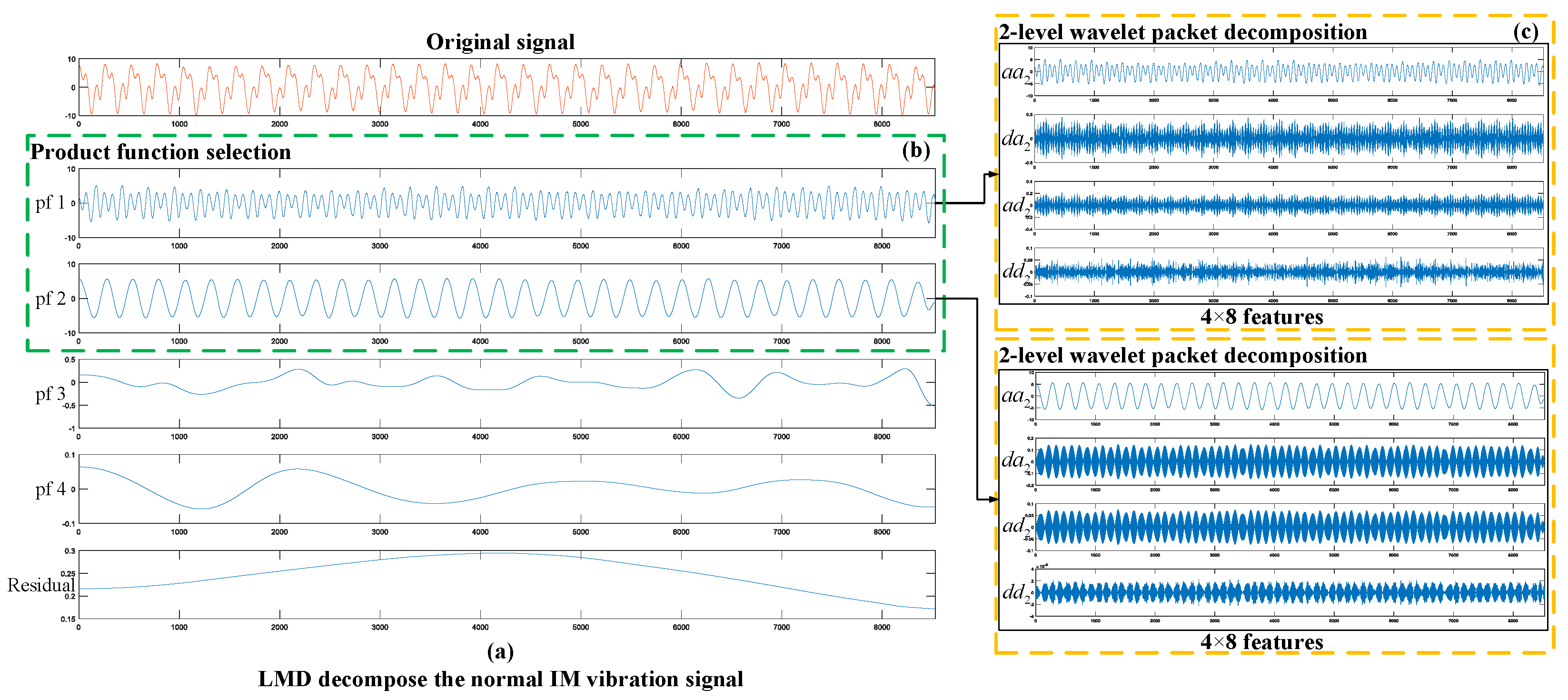
- In the first layer of the multilayer signal analysis, LMD is used to decompose the vibration signals into a set of PFs. Figure 1a illustrates how the LMD decomposes the normal IM vibration signal into four PFs.
- Step 3:
- In the second layer of the multilayer signal analysis, PF selection is used to select the effective components. In this paper, we choose the best two CEV values for the selected PFs into the final layer. Figure 1b illustrates the PF selection method selecting the best two PFs.
- Step 4:
- In the third layer of the multilayer signal analysis, WPD is used to further analyze and denoise the selected PFs. In this paper, two-level WPD is adopted and decomposition construction consists of four wavelet packet coefficients: , , , . The two-level WPD decomposes the selected PFs as shown in Figure 1c.
- Step 5:
- The eight statistical feature parameters are calculated for each wavelet packet coefficient. A total of 64 (2 × 4 × 8) features are extracted from the output decomposition structure of two selected PFs.
Therefore, the potential fault feature dataset includes 64 features. Table 1 shows the parameters definition of these statistical features.
3. Hybrid Genetic Binary Chicken Swarm Optimization for Feature Selection
This section can separate in four parts. The first part is a brief introduction to the basic BCSO algorithm for feature selection. The second to fourth parts explain each positions update strategy using the proposed HGBCSO method. The operation of these strategies combines with BCSO to search for a potential solution.
3.1. Binary Chicken Swarm Optimization
The basic CSO algorithm mimics the hierarchal order and behaviors of searching food in the chicken swarm. Each chicken is represented by their position in a -dimensional space by . The positions update of the equation of a different type of chickens is as follows:
- Rooster’s position update equation:where is a Gaussian distribution with a mean of 0 and standard deviation , is a small constant to prevent the denominator being 0. is a rooster’s index, which is selected randomly between 1 and the maximum number of roosters except . and are the fitness values of the ith and kth rooster.
- Hen’s position update equation:Rand is a uniform random number between 0 and 1, is an index of the rooster, which is in the ith hen’s group-mate, is an index of the chicken in all roosters and hens, which is randomly chosen from the swarm, and let .
- Chick’s position update equation:where is an index of the mother hen corresponding to ith chick, FL is a parameter in the range [0.4, 1], which keeps the chick to forage for food around its mother.
For feature selection in the BCSO, each chicken represents a solution in the binary search space (i.e., each feature subset). In contrast to CSO, each chicken is updated by the binary position of a solution which has values “1” and “0”, which means the corresponding feature is selected or unselected. The most widely used transfer function to transfer from the real position to the binary position is the sigmoid function in (17). The binary position of each chicken is updated as follows:
3.2. Update the Hen’s Position Based on Levy Flight
The disadvantage of basic CSO and other evolutionary algorithms is premature convergence. In basic CSO, hens play an important role in the entire group because there is the largest number of hens. Inspired by this, Liang et al. [30] proposed the levy flight search strategy into hen’s position update equation. In this method, the short-distance and occasional long-distance searching appear alternately, such that it enhances the search performance and avoids the iterations falling into a local optimal. The hen’s position update equation based on levy flight is as follows:
where ⊗ is a vector operator representing the point multiplication and the random step value of a levy flight is taken from the levy distribution, which is shown as follows:
3.3. Update the Chick’s Position Based on Inertia Weight
Based on CSO, the chicks’ do not update the position by themself, and only follow their own mother hen, so when their own mother hen falls into the local optimal, the chicks will also fall into the local optimal. In this research, the linear decreasing inertia weight is used to update the chick’s position, which can let the chicks update the position by themselves, preventing the chicks falling into local optimal. The linear decreasing inertia weight [52] updates as follows:
where and are the maximum and minimum values of inertia weight, is the number of iterations and is the maximum number of iterations. Then, the chick’s position update equation is defined as follows:
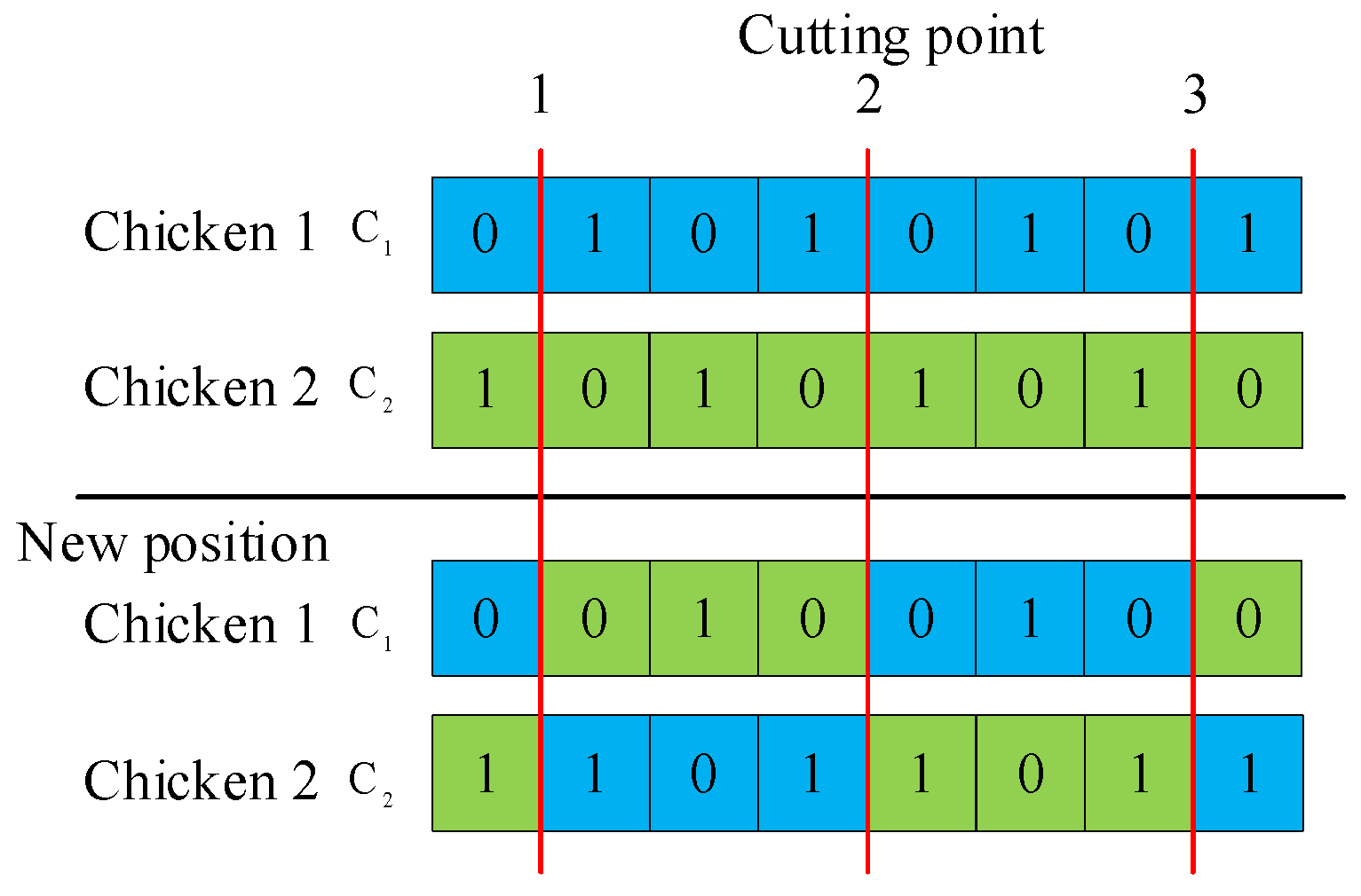
3.4. Update the Chicken’s Position Based on Crossover Operation
Based on GA: the crossover operation is a powerful tool for enhancing the exploration and exploitation capability, improving the population diversity, avoiding premature convergence, creating more effective solutions, and improving the average fitness values of the population. In this research, the chicken’s position update operation is based on three-points crossover operation. The operation is described as follows:
- Step 1:
- Randomly selected pairs of solutions carry out the three points crossover operation.
- Step 2:
- Repeat until the new population is formed.
The three-points crossover operation is illustrated in Figure 2.
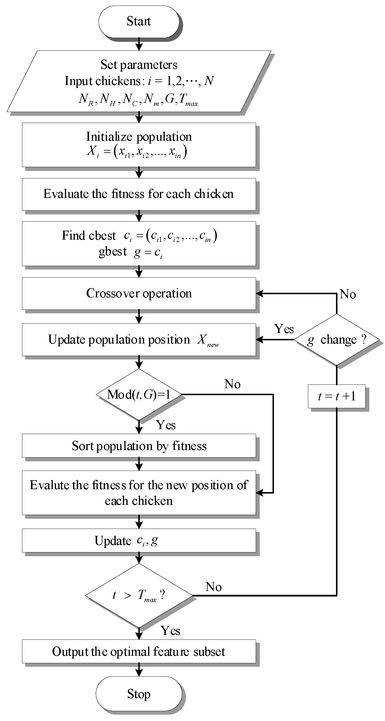
3.5. The Proposed HGBCSO Method
The proposed method HGBCSO is combined with the crossover operation and two positions update the strategies, which helps avoid the local optimal and improve the global search performance. Therefore, HGBCSO is the proposed method for feature selection in this research. The k-NN classifier is used to evaluate each chicken. The fitness function is based on the classification accuracy (ACC), which is defined as follows:
where is true positive, is false negative. The flowchart of the proposed method to achieve an optimal feature subset is illustrated in Figure 3.
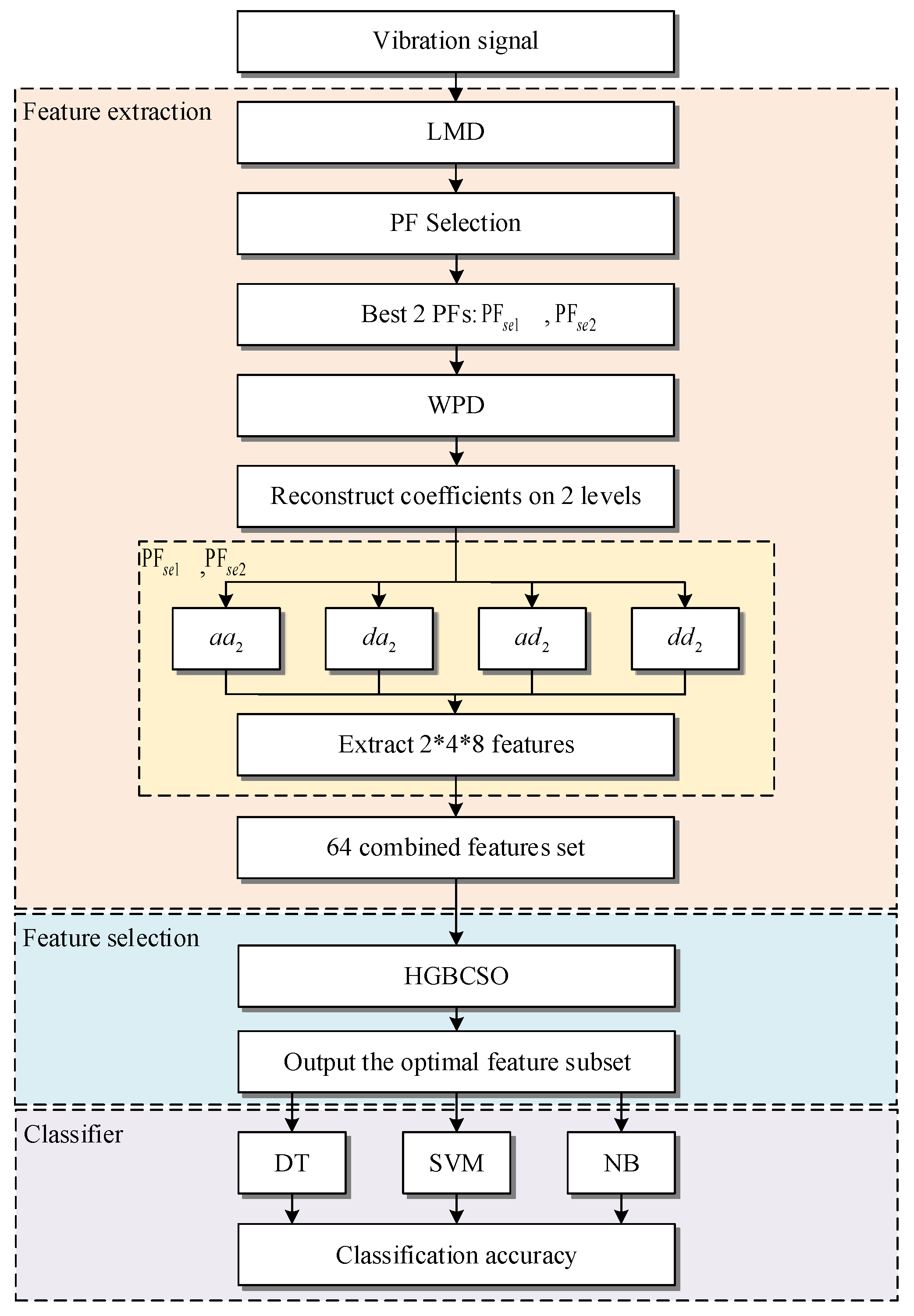
4. Diagnosis Model for Rotor Bar Fault
This section is introducing a fault diagnosis model for a rotor bar based on the vibration signals of the IM. Figure 4 illustrates the proposed model and contains the following three main stages:
- Stage 1:
- Measuring the vibration signals from the test IM, which are processed by multilayer signal analysis. The first layer is to use LMD to decompose the vibration signals into a set of PFs. The second layer is to use PF selection to select two effective PFs. The third layer is to use WPD to further analyze and denoise the selected PFs. In this model, the wavelet decomposition level is adopted at level 2. The eight statistical feature parameters are calculated for each wavelet packet coefficient. Finally, 64 features are extracted during Stage 1.
- Stage 2:
- Using the proposed method HGBCSO to remove the irrelative features from the feature set, achieving the optimal feature subset. The optimal feature subset will improve the classifier performance of the fault diagnosis model.
- Stage 3:
- Three well-known classifiers, including DT, SVM, and NB, are used to classify the optimal feature subset. The ACCs are used to evaluate the robustness of classifiers with rotor bar data to select the best classifier for diagnosing rotor bar faults.
5. Experiment Results
Two experimental case studies are introduced in this section.
Case study 1 shows the results of the HGBCSO method using the UCI machine learning datasets for feature selection. To evaluate the effectiveness of the HGBCSO method, the basic BCSO and two well-known evolutionary algorithms are compared.
Case study 2 uses the experimental dataset from IM, including normal motor and broken rotor bar motors, to evaluate the validity of the proposed model.
5.1. Case Study 1: UCI Machine Learning Datasets
- Describe of Datasets
The feature set used in the motor fault diagnosis model is usually the low-dimensional feature sets [53,54]. Thus, six UCI machine learning repository datasets [55] are applied in this research. The six machine learning datasets are described in Table 2.
- 2.
- Parameter Setting
In this research, the high ACC fault diagnosis model is our focus. The k-NN classifier with the number of nearest neighbor k = 1 and 10-folds cross-validation is adopted to evaluate the solutions from HGBCSO and the other three compared evolutionary algorithms. Table 3 shows the parameter setting of four algorithms, including HGBCSO, BCSO, BPSO, and BBA.
- 3.
- Experimental Results for UCI Machine Learning Datasets
This experiment was simulated by Matlab 2017a. The results of three algorithms, including BCSO, BPSO, and BBA are used to assess the validity of the proposed HGBCSO algorithm. In this experiment, two following indicators are using to compare the results of algorithms: (1) Convergence curve of the best solution for each algorithm; (2) Calculate the average ACC and the average number of selected features (Avg No. Fs) for each algorithm in thirty independent runs.
Figure 5 shows the convergence curve of the best solution for each algorithm. The HGBCSO achieves higher ACC than the other compared algorithms on leaf, vehicle silhouettes, WDBC, ionosphere, and sonar. Especially on WDBC and ionosphere, HGBCSO achieves higher ACC than the other compared algorithms of 1.17 and 1.14%. Table 4 presents the average fitness value (Avg fitness value) and the Avg No. Fs for each algorithm. In each dataset, the algorithm achieves better results which are in bold in Table 4. The results show that HGBCSO achieves a better average ACC in these six machine learning datasets. Especially on WDBC, the average classification accuracy is significantly better than BCSO with a difference of 1.56%. HGBCSO is most effective on the vehicle silhouettes and the ionosphere dataset achieves a higher Avg fitness value and lower Avg No. Fs. Based on the above results, the proposed HGBCSO method is satisfied with our focus.
5.2. Case Study 2: Rotor Broken Bar Experimental Database
- Experimental Setup
The experimental database for detecting and diagnosing rotor broken bar from the IEEE Dataport [56] was used in this case study. The experimental setup in this database consisted of a three-phase IM (1 hp, 220V/380V, 3.02A/1.75A, 4 poles, 60 Hz, a nominal torque of 4.1 Nm and a rated speed of 1715 rpm) coupled to a DC machine. To simulate the failure on the rotor, five rotors tested healthy for one, two, three, and four broken bars, respectively. In this experiment, 12.5, 50, and 100% of the full load of the experimental datasets were used in the rotor bar fault diagnosis model.
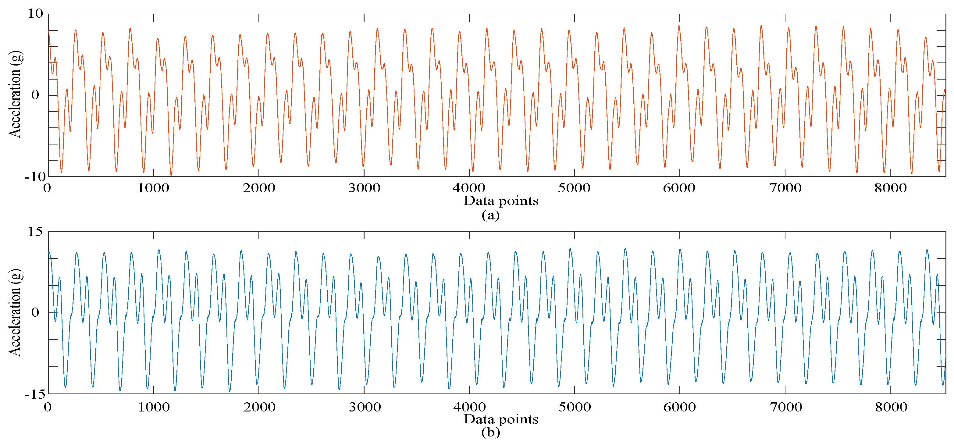
Five axial accelerometers (sensitivity of 10 mV/mm/s and the frequency range of 5 to 2000 Hz) were used to measure the vibration signals in both drive end (DE) and non-drive end (NDE) sides of the motor, axially or radially, in the horizontal or vertical directions. Vibration signals are acquired using a 10 channels data acquisition system with 16 bits A/D converters, type ADS 2000 Lynx Testing, and Measurement Systems. All vibration signals were sampled at the same time for 18 s, the sample rate of the vibration signals was 7.6 kHz, and ten repetitions were performed from the transient to steady state of the induction motor. Figure 6 shows the vibration signals acquisition from the healthy motor and broken bars motor.
- 2.
- Experimental Results for Feature Selection
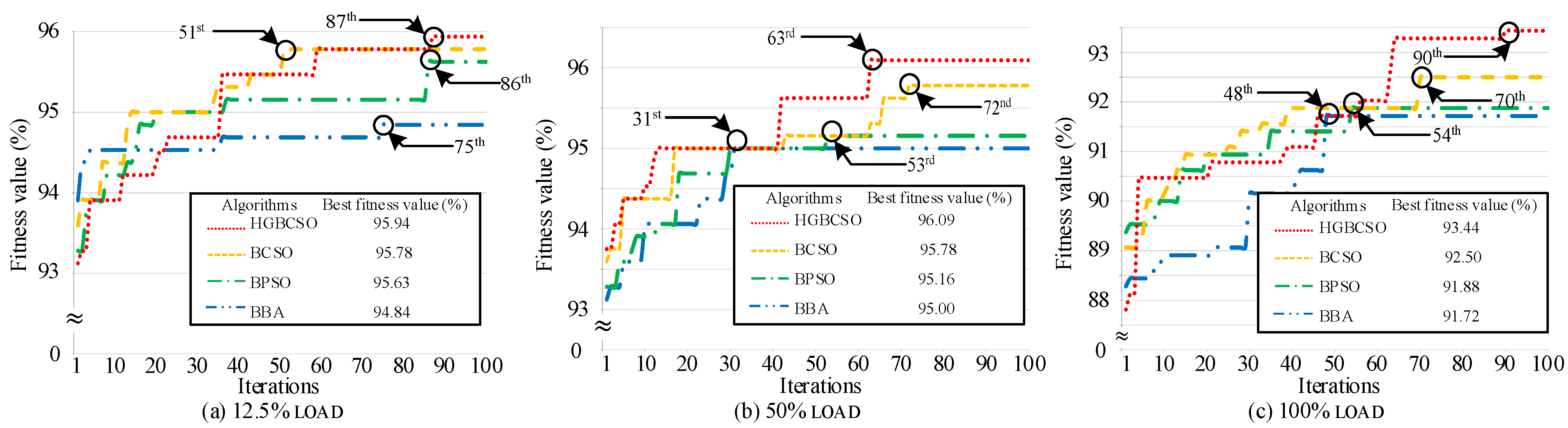
Section 4 presented the proposed three stages of the rotor bar fault diagnosis model. In stage 1, the potential fault feature dataset that included 64 features was extracted. In stage 2, HGBCSO was applied to the rotor bar datasets, including 12.5, 50, and 100% of full load conditions. In addition, the other three feature selection algorithms (BCSO, BPSO, BBA) are also calculated. The results under three different load conditions are shown from Table 5, Table 6 and Table 7. Compare with the other algorithms, the proposed algorithm reaches higher average classification accuracy in 30 independent runs. The convergence curves of the best solution under three different load conditions are shown in Figure 6. In Figure 7a, BCSO, BBA converge at the 51st and 75th iteration, respectively. In Figure 7b, BBA, BPSO converge at the 31st and 53rd iteration, respectively. In Figure 7c, BBA, BPSO converge at the 48th and 54th iteration, respectively. The above results show that the weaknesses of BCSO, BPSO, and BBA are its premature convergence and the likelihood of it falling into the local optimal. Meanwhile, in Figure 7a–c, HGBCSO converges at the 87th, 63rd, and 90th iteration, respectively. These results show that the proposed method based on three proposed positions’ update strategies has global exploration ability and preventing premature convergence.
Table 8, Table 9 and Table 10 present the best solution for each algorithm. Based on the number of the selected features of the optimal feature subset, HGBCSO has achieved 22 features from the 12.5% of full load condition dataset, 27 features from the 50% of full load condition dataset, and 23 features from the 100% of full-load condition dataset. Compared with the other algorithms, the proposed algorithm reaches the lower number of the selected features in 30 independent runs.
- 3.
- Experimental results for classification
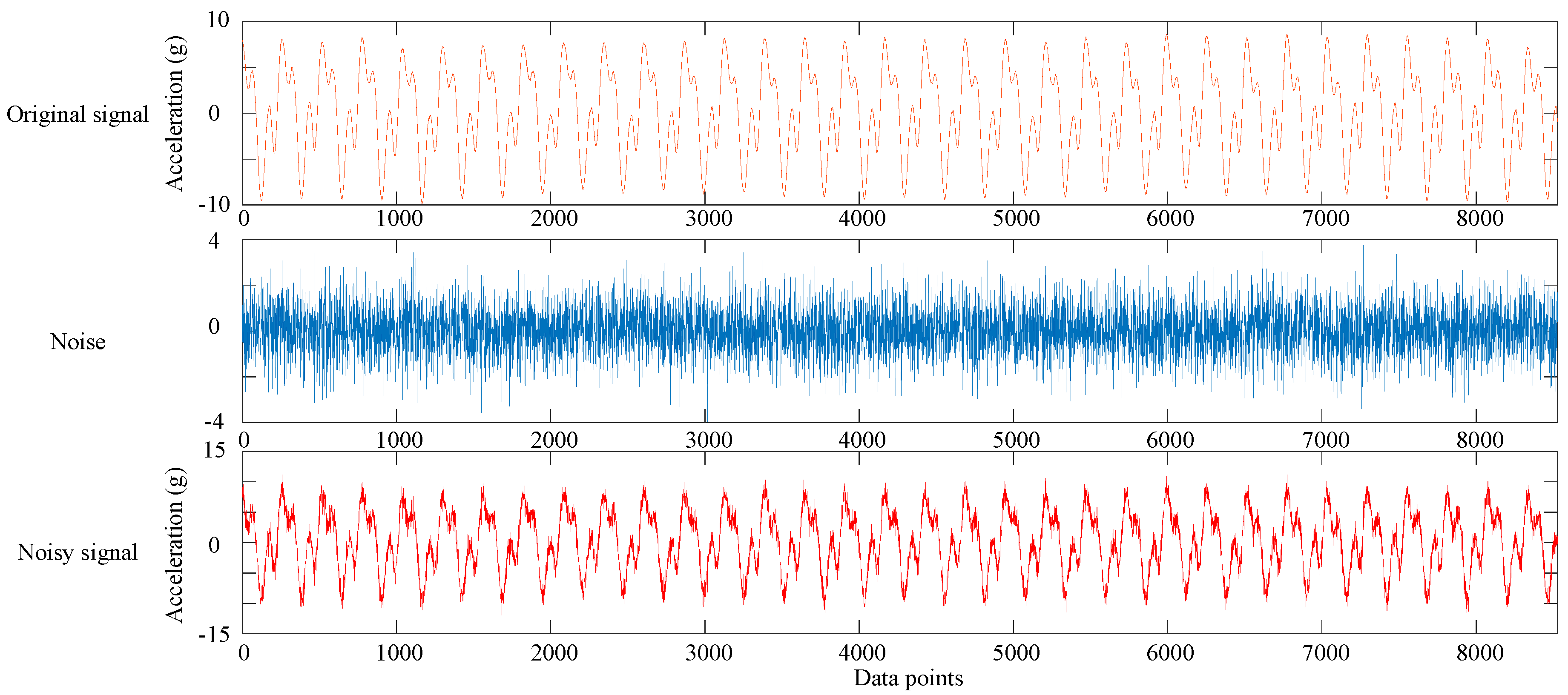
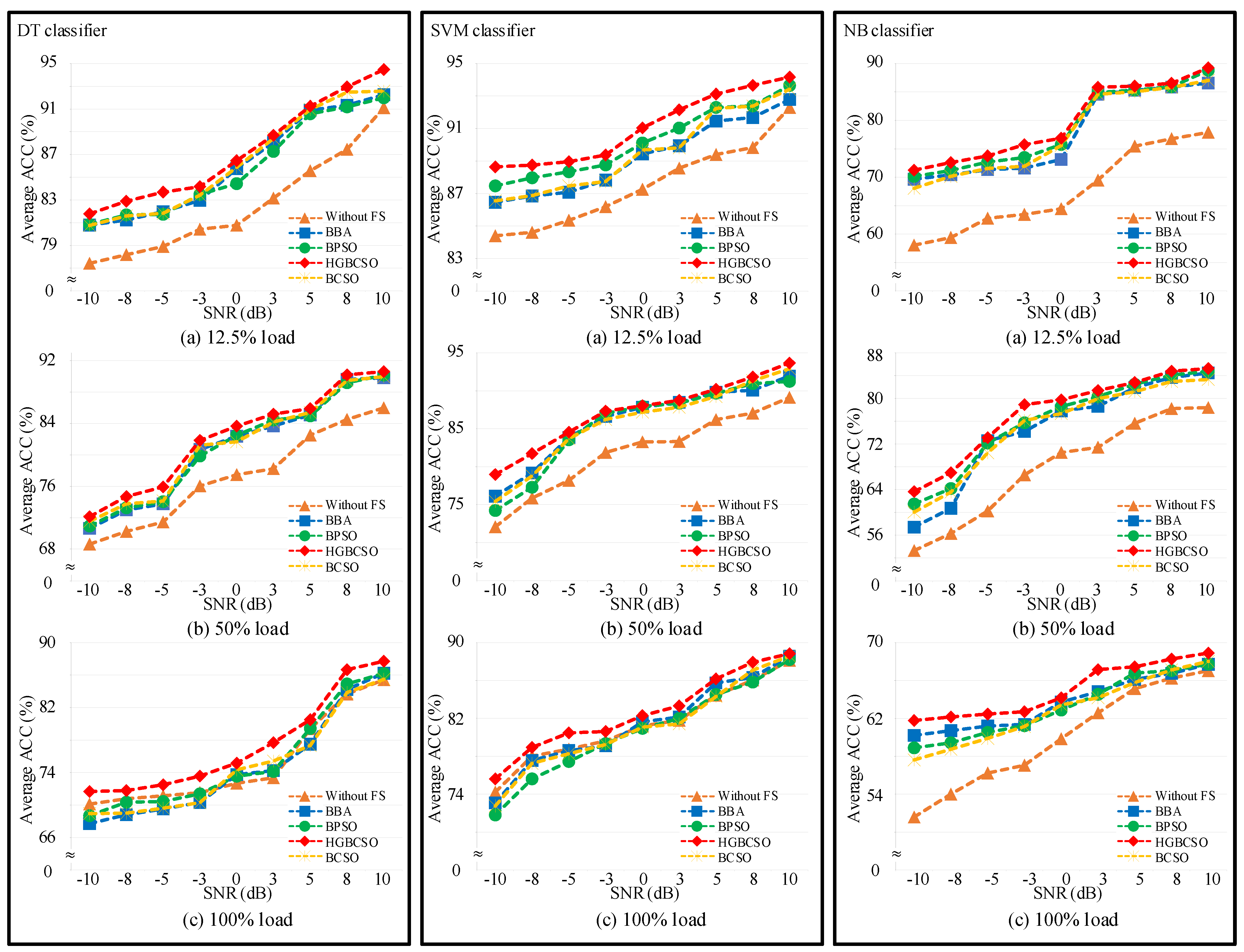
In stage 3, three provided classifiers, including DT, SVM, and NB, were adopted to classify the optimal feature subset. Table 11 shows the parameter setting of the three classifiers, including DT, SVM, and NB. Four optimal feature subsets were provided from HGBCSO, BCSO, BPSO, and BBA, respectively. In addition, the original feature set means without doing the feature selection were also used to classify in this experiment. The robustness of these three classifiers was also considered in the noise condition. In this experiment, the original signals were added to different levels of Gaussian white noise to simulate the noisy environment. This experiment was closer to the real condition in industrial production. In this experiment, the signal-to-noise ratio (SNR) value test ranged from −10 to 10 dB. Figure 8 shows the healthy motor signal is added by the Gaussian white noise with SNR = 0 dB. The average ACC is obtained after 30 training times. Figure 9 shows the average ACC using the DT, SVM, and NB of three different load conditions and under different SNR values. Obviously, DT and SVM achieved a better classification performance than NB. The proposed HGBCSO achieved higher ACC than the other three algorithms under different load conditions. As the SNR value decreases, the performance of the three classifiers decreases. However, under a lower SNR value, the robustness of the SVM classifier was more effective compared to DT and NB. Especially in SNR = −8 dB, the ACC of all algorithms and under 12.5, 50, and 100% of full load conditions are higher than 84.61, 75.86, and 75.62% when using the SVM classifier. The accuracy of all algorithms is lower than 82.89, 74.7, and 71.79% when using the DT classifier. The accuracy of all algorithms is lower than 72.6, 66.94, and 62.15% when using the NB classifier. In SNR = −10 dB, the ACC of SVM is still higher than DT and NB. Therefore, the SVM classifier is the suitable classifier with the rotor bar fault diagnosis model. Finally, we compared it with the classification results for different load conditions based on the proposed fault diagnosis model. As the load torque increases, the performance of the proposed model decreases. The classification accuracy of the proposed model under 12.5% of full load condition and under the SNR value ranging from −10 to 10 dB is from 88.64 to 94.17%. The classification accuracy of the proposed model under 50% of full load condition and under the SNR value ranging from −10 to 10 dB is from 78.97 to 93.67%, respectively. The classification accuracy of the proposed model under 100% of full load condition and under the SNR value ranging from −10 to 10 dB is from 75.62 to 88.83%. In conclusion, according to the above analysis, the proposed rotor bar fault diagnosis model in this research is highly effective and achieves high robustness to detecting rotor bar failure.
6. Conclusions
This article presents an effective rotor bar fault diagnosis model. The model contains three main stages to detect rotor bar failure. This research uses multilayer signal analysis for processing signals. In multilayer signal analysis, the vibration signals can be decomposed into the effective product function components which contains most of the fault information of the original signal. The proposed HGBCSO algorithm uses three positions update strategies to improve the basic BCSO algorithm and enhance the ability to select important features. The results show that the HGBCSO algorithm achieved higher ACC. The best fault diagnosis model achieves better robustness by using the SVM classifier. The classifier performance was tested from low load torque to full load torque and under high noise level. The result shows that the proposed model achieves 75.62% classification accuracy under 100% full load condition and SNR = −10 dB. In addition, the proposed HGBCSO algorithm was compared with the UCI machine learning datasets and the results are better than the adopted evolutionary algorithm. However, the proposed model still has some limitations as follows: (1) the feature extract process is highly dependent on the former knowledge for researchers; (2) machine learning has a shallow structure that cannot work well for complex non-linear problems. Therefore, deep learning algorithms and automatic feature extraction for rotor bar fault classification should be considered in the future.
Author Contributions
Conceptualization, C.-Y.L. and G.-L.Z.; methodology, C.-Y.L. and G.-L.Z.; software, C.-Y.L. and G.-L.Z.; validation, C.-Y.L. and G.-L.Z.; formal analysis, C.-Y.L. and G.-L.Z.; investigation, C.-Y.L. and G.-L.Z.; resources, C.-Y.L. and G.-L.Z.; data curation, C.-Y.L. and G.-L.Z.; writing—original draft preparation, G.-L.Z.; writing—review and editing, C.-Y.L.; visualization, C.-Y.L. and G.-L.Z.; supervision, C.-Y.L. and G.-L.Z.; project administration, C.-Y.L. and G.-L.Z.; funding acquisition, C.-Y.L. and G.-L.Z. Both authors have read and agreed to the published version of the manuscript.
Funding
This research received no external funding.
Institutional Review Board Statement
Not applicable.
Informed Consent Statement
Not applicable.
Data Availability Statement
Not applicable.
Conflicts of Interest
The authors declare no conflict of interest.
References
- Ola, E.H.; Amer, M.; Abdelsalam, A.K.; Williams, B.W. Induction motor broken rotor bar fault detection techniques based on fault signature analysis—A review. Electr. Power Appl. IET 2018, 12, 895–907. [Google Scholar]
- Garcia-Perez, A.; Ibarra-Manzano, O.; Romero-Troncoso, R.J. Analysis of partially broken rotor bar by using a novel empirical mode decomposition method. In Proceedings of the 40th Annual Conference of the IEEE Industrial Electronics Society, Dallas, TX, USA, 29 October–1 November 2014; pp. 3403–3408. [Google Scholar]
- Brkovic, A.; Gajic, D.; Gligorijevic, J.; Savic-Gajic, I.; Georgieva, O.; Di Gennaro, S. Early fault detection and diagnosis in bearings for more efficient operation of rotating machinery. Energy 2017, 136, 63–71. [Google Scholar] [CrossRef]
- Gligorijevic, J.; Gajic, D.; Brkovic, A.; Savic-Gajic, I.; Georgieva, O.; Di Gennaro, S. Online condition monitoring of bearings to support total productive maintenance in the packaging materials industry. Sensors 2016, 16, 316. [Google Scholar] [CrossRef] [Green Version]
- Van, M.; Kang, H.-J. Bearing-fault diagnosis using non-local means algorithm and empirical mode decomposition-based feature extraction and two-stage feature selection. IET Sci. Meas. Technol. 2015, 9, 671–680. [Google Scholar] [CrossRef]
- Helmi, H.; Forouzantabar, A. Rolling bearing fault detection of electric motor using time domain and frequency domain features extraction and ANFIS. IET Electr. Power Appl. 2019, 13, 662–669. [Google Scholar] [CrossRef]
- Singh, A.; Grant, B.; DeFour, R.; Sharma, C.; Bahadoorsingh, S. A review of induction motor fault modeling. Electr. Power Syst. Res. 2016, 133, 191–197. [Google Scholar] [CrossRef]
- Delgado-Arredondo, P.A.; Morinigo-Sotelo, D.; Osornio-Rios, R.A.; Avina-Cervantes, J.G.; Rostro-Gonzalez, H.; de Jesus Romero-Troncoso, R. Methodology for fault detection in induction motors via sound and vibration signals. Mech. Syst. Signal Process. 2017, 83, 568–589. [Google Scholar] [CrossRef]
- Yiyuan, G.; Dejie, Y.; Haojiang, W. Fault diagnosis of rolling bearings using weighted horizontal visibility graph and graph Fourier transform. Measurement 2020, 149, 107036. [Google Scholar]
- Fan, H.; Shao, S.; Zhang, X.; Wan, X.; Cao, X.; Ma, H. Intelligent fault diagnosis of rolling bearing using FCM clustering of EMD-PWVD vibration images. IEEE Access 2020, 8, 145194–145206. [Google Scholar] [CrossRef]
- Gao, M.; Yu, G.; Wang, T. Impulsive gear fault diagnosis using adaptive morlet wavelet filter based on alpha-stable distribution and kurtogram. IEEE Access 2019, 7, 72283–72296. [Google Scholar] [CrossRef]
- Pachori, R.B.; Nishad, A. Cross-terms reduction in the Wigner–Ville distribution using tunable-Q wavelet transform. Signal Process. 2016, 120, 288–304. [Google Scholar] [CrossRef]
- Huo, Z.; Zhang, Y.; Francq, P.; Shu, L.; Huang, J. Incipient fault diagnosis of roller bearing using optimized wavelet transform based multi-speed vibration signatures. IEEE Access 2017, 5, 19442–19456. [Google Scholar] [CrossRef] [Green Version]
- Minhas, A.S.; Singh, G.; Singh, J.; Kankar, P.K.; Singh, S. A novel method to classify bearing faults by integrating standard deviation to refined composite multi-scale fuzzy entropy. Measurement 2020, 154, 107441. [Google Scholar] [CrossRef]
- Huang, N.E.; Shen, Z.; Long, S.R.; Wu, M.C.; Shih, H.H.; Zheng, Q.; Yen, N.-C.; Tung, C.C.; Liu, H.H. The empirical mode decomposition and the Hilbert spectrum for nonlinear and non-stationary time series analysis. Proc. R. Soc. Lond. Ser. A 1998, 454, 903–995. [Google Scholar] [CrossRef]
- Wu, Z.H.; Huang, N.E. Ensemble empirical mode decomposition: A noise-assisted data analysis method. Adv. Adapt. Data Anal. 2009, 1, 1–41. [Google Scholar] [CrossRef]
- Li, P.; Gao, J.; Xu, D.; Wang, C.; Yang, X. Hilbert-Huang transform with adaptive waveform matching extension and its application in power quality disturbance detection for microgrid. J. Mod. Power Syst. Clean Energy 2016, 4, 19–27. [Google Scholar] [CrossRef] [Green Version]
- Zhang, X.; Liu, Z.; Miao, Q.; Wang, L. An optimized time varying filtering based empirical mode decomposition method with grey wolf optimizer for machinery fault diagnosis. J. Sound Vib. 2018, 418, 55–78. [Google Scholar] [CrossRef]
- Smith, J.S. The local mean decomposition and its application to EEG perception data. J. R. Soc. Inter. 2005, 2, 443–454. [Google Scholar] [CrossRef] [PubMed]
- Wang, Y.; He, Z.; Zi, Y. A Comparative Study on the Local Mean Decomposition and Empirical Mode Decomposition and Their Applications to Rotating Machinery Health Diagnosis. ASME J. Vib. Acoust. 2010, 132, 021010. [Google Scholar] [CrossRef]
- Cheng, J.; Yang, Y.; Yang, Y. A rotating machinery fault diagnosis method based on local mean decomposition. Dig. Signal Process. 2012, 22, 356–366. [Google Scholar] [CrossRef]
- Guo, W.; Huang, L.; Chen, C.; Zou, H.; Liu, Z. Elimination of end effects in local mean decomposition using spectral coherence and applications for rotating machinery. Dig. Signal Process. 2016, 55, 52–63. [Google Scholar] [CrossRef]
- Wang, Y.; Xu, G.; Liang, L.; Jiang, K. Detection of weak transient signals based on wavelet packet transform and manifold learning for rolling element bearing fault diagnosis. Mech. Syst. Signal Process. 2015, 54–55, 259–276. [Google Scholar] [CrossRef]
- Shao, R.; Hu, W.; Wang, Y.; Qi, X. The fault feature extraction and classification of gear using principal component analysis and kernel principal component analysis based on the wavelet packet transform. Measurement 2014, 54, 118–132. [Google Scholar] [CrossRef]
- Sun, J.; Xiao, Q.; Wen, J.; Wang, F. Natural gas pipeline small leakage feature extraction and recognition based on LMD envelope spectrum entropy and SVM. Measurement 2014, 55, 434–443. [Google Scholar] [CrossRef]
- Ang, J.C.; Mirzal, A.; Haron, H.; Hamed, H.N.A. Supervised, unsupervised, and semi-supervised feature selection: A review on gene selection. IEEE/ACM Trans. Comput. Biol. Bioinf. 2016, 13, 971–989. [Google Scholar] [CrossRef] [PubMed]
- Meng, X.-B.; Gao, X.Z.; Liu, Y.; Zhang, H. A novel bat algorithm with habitat selection and Doppler effect in echoes for optimization. Expert Syst. Appl. 2015, 42, 6350–6364. [Google Scholar] [CrossRef]
- Karim, A.A.; Isa, N.A.M.; Lim, W.H. Modified particle swarm optimization with effective guides. IEEE Access 2020, 8, 188699–188725. [Google Scholar] [CrossRef]
- Meng, X.; Liu, Y.; Gao, X.; Zhang, H. A new bio-inspired algorithm: Chicken swarm optimization. In Advances in Swarm Intelligence (Lecture Notes in Computer Science); Springer: Cham, Switzerland, 2014; Volume 8794, pp. 86–94. [Google Scholar]
- Liang, X.; Kou, D.; Wen, L. An improved chicken swarm optimization algorithm and its application in robot path planning. IEEE Access 2020, 8, 49543–49550. [Google Scholar] [CrossRef]
- Qu, C.; Zhao, S.; Fu, Y.; He, W. Chicken swarm optimization based on elite opposition-based learning. Math. Probl. Eng. 2017, 2017, 1–20. [Google Scholar] [CrossRef]
- Liang, S.; Fang, Z.; Sun, G.; Liu, Y.; Qu, G.; Zhang, Y. Sidelobe reductions of antenna arrays via an improved chicken swarm optimization approach. IEEE Access 2020, 8, 37664–37683. [Google Scholar] [CrossRef]
- Lee, C.-Y.; Le, T.-A. Optimised approach of feature selection based on genetic and binary state transition algorithm in the classification of bearing fault in BLDC motor. IET Electr. Power Appl. 2020, 14, 2598–2608. [Google Scholar] [CrossRef]
- Xue, B.; Zhang, M.; Browne, W.N.; Yao, X. A survey on evolutionary computation approaches to feature selection. IEEE Trans. Evol. Comput. 2016, 20, 606–626. [Google Scholar] [CrossRef] [Green Version]
- Kennedy, J.; Eberhart, R.C. A discrete binary version of the particle swarm algorithm. In Proceedings of the IEEE International Conference on Systems, Man and Cybernetics, Orlando, FL, USA, 12–15 October 1997; pp. 4104–4108. [Google Scholar]
- Nakamura, R.Y.M.; Pereira, L.A.M.; Rodrigues, D.; Costa, K.A.P.; Papa, J.P.; Yang, X.-S. 9—Binary bat algorithm for feature selection. In Swarm Intelligence and Bio-Inspired Computation; Elsevier: Amsterdam, The Netherlands, 2013; pp. 225–237. [Google Scholar]
- Liu, F.; Yan, X.; Lu, Y. Feature selection for image steganalysis using binary bat algorithm. IEEE Access 2019, 8, 4244–4249. [Google Scholar] [CrossRef]
- Ahmed, K.; Hassanien, A.E.; Bhattacharyya, S. A novel chaotic chicken swarm optimization algorithm for feature selection. In Proceedings of the 3rd International Conference on Research in Computational Intelligence and Communication Networks (ICRCICN), Kolkata, India, 3–5 November 2017; pp. 259–264. [Google Scholar]
- Hafez, A.I.; Zawbaa, H.M.; Emary, E.; Mahmoud, H.A.; Hassanien, A.E. An innovative approach for feature selection based on chicken swarm optimization. In Proceedings of the 7th International Conference of Soft Computing and Pattern Recognition (SoCPaR), Fukuoka, Japan, 13–15 November 2015; pp. 19–24. [Google Scholar]
- Long, J.; Zhang, S.; Li, C. Evolving deep echo state networks for intelligent fault diagnosis. IEEE Trans. Ind. Inform. 2020, 16, 4928–4937. [Google Scholar] [CrossRef]
- Lee, C.-Y.; Le, T.-A. Intelligence bearing fault diagnosis model using multiple feature extraction and binary particle swarm optimization with extended memory. IEEE Access 2020, 8, 198343–198356. [Google Scholar] [CrossRef]
- De Giorgi, M.G.; Ficarella, A.; Lay-Ekuakille, A. Cavitation regime detection by LS-SVM and ANN with wavelet decomposition based on pressure sensor signals. IEEE Sens. J. 2015, 15, 5701–5708. [Google Scholar] [CrossRef]
- Sunny; Kumar, V.; Mishra, V.N.; Dwivedi, R.; Das, R.R. Classification and quantification of binary mixtures of gases/odors using thick-film gas sensor array responses. IEEE Sens. J. 2015, 15, 1252–1260. [Google Scholar] [CrossRef]
- Shamshirband, S.; Petković, D.; Javidnia, H.; Gani, A. Sensor data fusion by support vector regression methodology—A comparative study. IEEE Sens. J. 2015, 15, 850–854. [Google Scholar] [CrossRef]
- De Giorgi, M.G.; Congedo, P.M.; Malvoni, M.; Laforgia, D. Error analysis of hybrid photovoltaic power forecasting models: A case study of mediterranean climate. Energy Convers. Manag. 2015, 100, 117–130. [Google Scholar] [CrossRef]
- Lei, Y.; Yang, B.; Jiang, X.; Jia, F.; Li, N.; Nandi, A.K. Applications of machine learning to machine fault diagnosis: A review and roadmap. Mech. Syst. Signal Process. 2020, 138, 106587. [Google Scholar] [CrossRef]
- Meng, L.; Xiang, J.; Wang, Y.; Jiang, Y.; Gao, H. A hybrid fault diagnosis method using morphological filter–translation invariant wavelet and improved ensemble empirical mode decomposition. Mech. Syst. Signal Process. 2015, 50–51, 101–115. [Google Scholar] [CrossRef]
- Lei, Y.; Li, N.; Lin, J. A new method based on stochastic process models for machine remaining useful life prediction. IEEE Trans. Instrum. Meas. 2016, 65, 2671–2684. [Google Scholar] [CrossRef]
- Xu, F.; Song, X.; Tsui, K.; Yang, F.; Huang, Z. Bearing performance degradation assessment based on ensemble empirical mode decomposition and affinity propagation clustering. IEEE Access 2019, 7, 54623–54637. [Google Scholar] [CrossRef]
- Yu, J.; Lv, J. Weak fault feature extraction of rolling bearings using local mean decomposition-based multilayer hybrid denoising. IEEE Trans. Instrum. Meas. 2017, 66, 3148–3159. [Google Scholar] [CrossRef]
- Xian, G.-M.; Zeng, B.-Q. An intelligent fault diagnosis method based on wavelet packer analysis and hybrid support vector machines. Expert Syst. Appl. 2009, 36, 12131–12136. [Google Scholar] [CrossRef]
- Bansal, J.C.; Singh, P.K.; Saraswat, M.; Verma, A.; Jadon, S.S.; Abraham, A. Inertia weight strategies in particle swarm optimization. In Proceedings of the 2011 IEEE World Congress on Nature and Biologically Inspired Computing, Salamanca, Spain, 19–21 October 2011; pp. 633–640. [Google Scholar]
- He, Y.; Hu, M.; Feng, K.; Jiang, Z. An intelligent fault diagnosis scheme using transferred samples for intershaft bearings under variable working conditions. IEEE Access 2020, 8, 203058–203069. [Google Scholar] [CrossRef]
- Van, M.; Kang, H. Wavelet kernel local fisher discriminant analysis with particle swarm optimization algorithm for bearing defect classification. IEEE Trans. Instrum. Meas. 2015, 64, 3588–3600. [Google Scholar] [CrossRef]
- UCI Machine Learning Repository. Available online: http://archive.ics.uci.edu/ml (accessed on 5 September 2020).
- Treml, A.E.; Flauzino, R.A.; Suetake, M.; Maciejewski, N.A.R. Experimental database for detecting and diagnosing rotor broken bar in a three-phase induction motor. IEEE DataPort 2020. [Google Scholar] [CrossRef]
Figure 1.
The graphics of the feature extraction process. (a) LMD decomposes the vibration signal (b) PF selection method (c) two-level WPD.
Figure 1.
The graphics of the feature extraction process. (a) LMD decomposes the vibration signal (b) PF selection method (c) two-level WPD.

Figure 2.
Three-points crossover operation.

Figure 3.
The flowchart of the proposed hybrid genetic binary chicken swarm optimization (HGBCSO) method.
Figure 3.
The flowchart of the proposed hybrid genetic binary chicken swarm optimization (HGBCSO) method.

Figure 4.
The flowchart of diagnosis model for rotor bar fault.

Figure 5.
Convergence curves for HGBCSO and other evolutionary algorithms in six datasets. (a) Wine (b) Leaf (c) Vehicle Silhouettes (d) WDBC (e) Ionosphere (f) Sonar.
Figure 5.
Convergence curves for HGBCSO and other evolutionary algorithms in six datasets. (a) Wine (b) Leaf (c) Vehicle Silhouettes (d) WDBC (e) Ionosphere (f) Sonar.

Figure 6.
Acquisition for collecting data from accelerometers: (a) healthy; and (b) broken bars.

Figure 7.
Convergence curve of the best solution for different load conditions in three datasets. (a) 12.5% Load(b) 50% Load (c) 100% Load.
Figure 7.
Convergence curve of the best solution for different load conditions in three datasets. (a) 12.5% Load(b) 50% Load (c) 100% Load.

Figure 8.
The illustration adding white Gaussian noise into the original signal.

Figure 9.
Comparison of three classifier performances with different SNR values in three datasets. (a) 12.5% Load (b) 50% Load (c) 100% Load.
Figure 9.
Comparison of three classifier performances with different SNR values in three datasets. (a) 12.5% Load (b) 50% Load (c) 100% Load.


Table 1.
Eight statistical feature definition.
| Feature | Equation |
|---|---|
| (1) Max value | |
| (2) Min value | |
| (3) Root mean square | |
| (4) Mean square error | |
| (5) Standard deviation | |
| (6) Kurtosis | |
| (7) Crest factor | |
| (8) Clearance factor |
Note: x(n) is a signal series for , where N is the number of data points.
Table 2.
Description of 6 UCI machine learning datasets.
| Datasets | Features | Instances | Classes |
|---|---|---|---|
| Wine | 13 | 178 | 3 |
| Leaf | 15 | 340 | 30 |
| Vehicle Silhouettes | 18 | 94 | 4 |
| WDBC | 30 | 569 | 2 |
| Ionosphere | 34 | 351 | 2 |
| Sonar | 60 | 208 | 2 |
Table 3.
Experimental parameter setting of four evolutionary algorithms.
| HGBCSO | BCSO | BPSO | BBA |
|---|---|---|---|
| Number of chickens: 10 Number of iterations: 100 Rooster parameter: 0.2 Hen parameter: 0.7 Mother parameter: 0.1 ωmin = 0.4 ωmax = 0.9 | Number of chickens: 10 Number of iterations: 100 Rooster parameter: 0.2 Hen parameter: 0.7 Mother parameter: 0.1 | Number of particles: 10 Number of iterations: 100 c1 = c2 = 2.05 | Number of bats: 10 Number of iterations: 100 Maximum frequency: 2 Minimum frequency: 0 Loudness: 0.9 Pulse rate: 0.9 |
Table 4.
The result of HGBCSO and other evolutionary algorithms.
| Datasets | HGBCSO | BCSO | BPSO | BBA | ||||
|---|---|---|---|---|---|---|---|---|
| Avg Fitness Value | Avg No. Fs | Avg Fitness Value | Avg No. Fs | Avg Fitness Value | Avg No. Fs | Avg Fitness Value | Avg No. Fs | |
| Wine | 99.53 | 8.93 | 99.49 | 8.60 | 99.06 | 8.37 | 98.29 | 7.77 |
| Leaf | 76.25 | 10.73 | 76.07 | 10.73 | 75.16 | 10.43 | 72.45 | 9.2 |
| Vehicle Silhouettes | 76.60 | 8.33 | 75.99 | 9.17 | 74.61 | 9.37 | 71.21 | 9.57 |
| WDBC | 99.37 | 16.23 | 97.81 | 16.30 | 97.45 | 15.60 | 96.83 | 15.90 |
| Ionosphere | 94.19 | 13.23 | 93.76 | 14.3 | 93.23 | 14.77 | 91.72 | 15.7 |
| Sonar | 94.37 | 31.07 | 93.53 | 31.13 | 93.33 | 31.43 | 90.51 | 30.43 |
Table 5.
Comparison of the 12.5% load condition rotor bar dataset.
| Algorithms | Avg Fitness Value (%) | Avg No. Fs |
|---|---|---|
| HGBCSO | 95.09 | 31.73 |
| BCSO | 95.05 | 31.97 |
| BPSO | 93.99 | 32.80 |
| BBA | 94.57 | 32.83 |
Table 6.
Comparison of the 50% load condition rotor bar dataset.
| Algorithms | Avg Fitness Value (%) | Avg No. Fs |
|---|---|---|
| HGBCSO | 95.22 | 28.6 |
| BCSO | 95.09 | 30.27 |
| BPSO | 94.64 | 33.03 |
| BBA | 94.22 | 32.70 |
Table 7.
Comparison on the 100% load condition rotor bar dataset.
| Algorithms | Avg Fitness Value (%) | Avg No. Fs |
|---|---|---|
| HGBCSO | 91.86 | 29.10 |
| BCSO | 91.70 | 30.67 |
| BPSO | 90.83 | 31.50 |
| BBA | 89.85 | 31.57 |
Table 8.
Details on the 12.5% load condition rotor bar dataset.
| Algorithms | Features | Feature Indicators (F) |
|---|---|---|
| HGBCSO | 22 | 2, 3, 5, 9, 10, 12, 14, 15, 16, 17, 18, 19, 20, 22, 29, 30, 41, 44, 47, 49, 51, 55. |
| BCSO | 28 | 1, 2, 3, 5, 7, 8, 9, 11, 12, 13, 14, 15, 16, 17, 20, 23, 26, 27, 29, 30, 32, 40, 41, 46, 51, 52, 55, 58. |
| BPSO | 31 | 2, 3, 5, 8, 9, 11, 12, 13, 15, 16, 17, 18, 19, 20, 22, 25, 26, 27, 28, 29, 30, 31, 32, 33, 38, 41, 45, 46, 50, 51, 63. |
| BBA | 32 | 2, 3, 4, 8, 9, 11, 12, 13, 14, 15, 16, 18, 19, 20, 22, 24, 26, 27, 30, 32, 33, 35, 36, 38, 40, 41, 42, 44, 45, 49, 54, 63. |
Table 9.
Details on the 50% load condition rotor bar dataset.
| Algorithms | Features | Feature Indicators (F) |
|---|---|---|
| HGBCSO | 27 | 1, 5, 6, 7, 9, 10, 11, 12, 13, 14, 19, 20, 21, 22, 24, 25, 26, 28, 31, 33, 36, 39, 40, 42, 48, 53, 61. |
| BCSO | 38 | 1, 3, 4, 8, 9, 10, 11, 12, 13, 14, 15, 16, 17, 19, 20, 21, 23, 24, 25, 31, 32, 33, 35, 37, 38, 39, 42, 43, 46, 47, 50, 51, 52, 53, 55, 57, 61, 63. |
| BPSO | 30 | 1, 6, 7, 8, 9, 10, 11, 12, 13, 15, 17, 18, 19, 20, 22, 24, 27, 31, 37, 38, 39, 42, 43, 44, 46, 48, 49, 50, 52, 55. |
| BBA | 32 | 1, 3, 4, 7, 8, 9, 10, 11, 12, 13, 14, 16, 18, 20, 22, 25, 27, 29, 31, 34, 35, 36, 38, 39, 40, 45, 48, 51, 54, 56, 58, 60. |
Table 10.
Details on the 100% load condition rotor bar dataset.
| Algorithms | Features | Feature Indicators (F) |
|---|---|---|
| HGBCSO | 23 | 1, 2, 4, 5, 10, 12, 15, 16, 17, 18, 19, 20, 22, 23, 24, 37, 38, 41, 42, 43, 44, 46, 52. |
| BCSO | 33 | 5, 6, 8, 10, 12, 13, 14, 15, 16, 17, 18, 19, 20, 22, 23, 24, 25, 27, 32, 33, 37, 40, 41, 43, 44, 45, 49, 51, 52, 53, 56, 61, 63. |
| BPSO | 33 | 3, 5, 6, 8, 9, 10, 11, 12, 14, 16, 17, 19, 20, 21, 22, 23, 25, 27, 28, 36, 37, 42, 44, 47, 49, 50, 52, 53, 54, 55, 59, 61, 63. |
| BBA | 34 | 3, 4, 5, 6, 8, 9, 10, 11, 12, 13, 15, 17, 18, 19, 20, 22, 23, 25, 26, 28, 32, 33, 36, 37, 39, 41, 42, 45, 46, 50, 53, 54, 59, 62. |
Table 11.
Parameter setting of three classifiers.
| DT | SVM | NB |
|---|---|---|
| Complex tree Split criterion: Gini’s diversity index Surrogate splits: off Max number of splits: 100 | Kernel function: polynomial Polynomial order: 2 Kernel scale: auto Box constraint: 1 | Kernel distributions: normal Support regions: unbounded |
Publisher’s Note: MDPI stays neutral with regard to jurisdictional claims in published maps and institutional affiliations. |
© 2021 by the authors. Licensee MDPI, Basel, Switzerland. This article is an open access article distributed under the terms and conditions of the Creative Commons Attribution (CC BY) license (http://creativecommons.org/licenses/by/4.0/).
Share and Cite
MDPI and ACS Style
Lee, C.-Y.; Zhuo, G.-L. Effective Rotor Fault Diagnosis Model Using Multilayer Signal Analysis and Hybrid Genetic Binary Chicken Swarm Optimization. Symmetry 2021, 13, 487. https://0-doi-org.brum.beds.ac.uk/10.3390/sym13030487
AMA Style
Lee C-Y, Zhuo G-L. Effective Rotor Fault Diagnosis Model Using Multilayer Signal Analysis and Hybrid Genetic Binary Chicken Swarm Optimization. Symmetry. 2021; 13(3):487. https://0-doi-org.brum.beds.ac.uk/10.3390/sym13030487
Chicago/Turabian StyleLee, Chun-Yao, and Guang-Lin Zhuo. 2021. "Effective Rotor Fault Diagnosis Model Using Multilayer Signal Analysis and Hybrid Genetic Binary Chicken Swarm Optimization" Symmetry 13, no. 3: 487. https://0-doi-org.brum.beds.ac.uk/10.3390/sym13030487
Note that from the first issue of 2016, this journal uses article numbers instead of page numbers. See further details here.