Nonequilibrium Dynamics of the Chiral Quark Condensate under a Strong Magnetic Field

Abstract

Strong magnetic fields impact quantum-chromodynamics (QCD) properties in several situations; examples include the early universe, magnetars, and heavy-ion collisions. These examples share a common trait—time evolution. A prominent QCD property impacted by a strong magnetic field is the quark condensate, an approximate order parameter of the QCD transition between a high-temperature quark-gluon phase and a low-temperature hadronic phase. We use the linear sigma model with quarks to address the quark condensate time evolution under a strong magnetic field. We use the closed time path formalism of nonequilibrium quantum field theory to integrate out the quarks and obtain a mean-field Langevin equation for the condensate. The Langevin equation features dissipation and noise kernels controlled by a damping coefficient. We compute the damping coefficient for magnetic field and temperature values achieved in peripheral relativistic heavy-ion collisions and solve the Langevin equation for a temperature quench scenario. The magnetic field changes the dissipation and noise pattern by increasing the damping coefficient compared to the zero-field case. An increased damping coefficient increases fluctuations and time scales controlling condensate’s short-time evolution, a feature that can impact hadron formation at the QCD transition. The formalism developed here can be extended to include other order parameters, hydrodynamic modes, and system’s expansion to address magnetic field effects in complex settings as heavy-ion collisions, the early universe, and magnetars.

1. Introduction

Strong magnetic fields impact prominent quantum-chromodynamics (QCD) phenomena, notably those associated with QCD’s approximate chiral symmetry in the light-quark sector. Special in this respect is the impact on the chiral condensate, as revealed by recent lattice QCD calculations [1,2,3]. The chiral condensate is an approximate order parameter for the finite temperature QCD transition between a high-temperature quark-gluon phase (QGP) and a low-temperature hadronic phase. The transition likely qualifies as a crossover (not a phase transition), in that the chiral condensate is nearly zero in the QGP phase, and nonzero in the hadronic phase, with a rapid change (not a jump) around the pseudocritical temperature $T_{\mathrm{pc}}\simeq 150$ MeV [4]. Such a rapid change in the condensate’s value is key to our understanding of how protons and neutrons (and other light-flavor hadrons) acquire their masses from almost massless quarks and gluons [5,6]. Phenomenologically, QCD matter under strong magnetic fields occurs in different settings, to name three of great current interest—the early universe [7,8], magnetars [9,10], and relativistic heavy-ion collisions [11,12]. Magnetized QCD matter in those settings evolves in time, albeit under very different time scales. A QGP to hadron transition occurring under such circumstances typifies a nonequilibrium phase change problem. In this paper, we present a first study of such a dynamical transition in magnetized QCD matter; to wit: we study the nonequilibrium dynamics of the chiral condensate under a strong magnetic field.

Magnetic field strengths and space-time scales in this study concern the phenomenology related to high-energy heavy-ion collision experiments. Relativistic heavy-ion collisions produce QCD matter of deconfined quarks and gluons, the quark-gluon plasma (QGP). Noncentral collisions produce the QGP under strong magnetic fields [11,12]; for example, noncentral Pb-Pb collisions at the Large Hadron Collider (LHC) can produce fields of strengths as large as [13] $eB=15m_{\pi }^2$. We conduct our study within the perspective of a standard three-stage scenario of QGP’s time evolution [14,15,16,17]: (1) quarks and gluons are freed from the protons and neutrons of the colliding ions and form (2) hot matter that expands hydrodynamically until it (3) cools up to a temperature $T\sim 150$ MeV, and finally disassembles into hadrons. More specifically, we work within the perspective that local thermodynamic properties as temperature and order parameter acquire physical meaning.

We address magnetic field effects on the chiral condensate dynamics with Langevin field equations, equations widely used in field theory treatments of dynamical phase transitions [18,19]. A prototype dynamical transition addressed by these equations is the one of a temperature quench in a spin system, in that a sudden drop in the system’s temperature takes the system out from a spin-disordered phase and drives it irreversibly toward a spin-ordered phase. The quench-induced transition just described resembles, albeit with differences, the heavy-ion collision evolution across the crossover from a quark-gluon phase, in which the condensate is very small, toward a hadron-dominated phase, in which the condensate ultimately reaches its vacuum value. Indeed, for zero magnetic field, there is a vast literature on the use of Langevin field equations in this context—References [20,21,22,23,24,25,26,27,28,29,30,31,32,33,34,35,36,37,38,39] are a sample of this literature. The Langevin equations featured in that literature are either postulated on phenomenological grounds [23,26,33,34,35,39], or derived from a microscopic model through a coarse-graining procedure [20,21,22,24,25,27,28,29,30,31,32,36,37,38]. We follow the latter approach.

We extend the semiclassical approach of Reference [29] to include magnetic field effects on the chiral condensate dynamics. In that approach, the condensate dynamics is governed by a Langevin field equation derived from a semiclassical two-particle irreducible (2PI) effective action. The effective action, computed with the time path formalism of nonequilibrium quantum field theory [40,41], refers to the Gell-Mann–Levy linear sigma model [42] with quarks (LSMq). The LSMq features degrees of freedom associated with the long-wavelength QCD chiral physics—constituent quarks, pseudoscalar-isoscalar mesons (pions, pseudo-Goldstone bosons) and a scalar-isoscalar meson (the quark condensate). The model does not describe quark confinement. Despite of this limitation, the model describes many of the equilibrium, time-independent magnetic field effects on the QCD equation of state, phase structure and chiral condensate [43,44,45,46,47,48,49,50,51,52,53,54,55] brought out by lattice calculations. We direct the reader to References [56,57,58,59] for reviews with additional references on works employing the LSMq and also other models.

This first study aims primarily to get insight into how a strong magnetic field affects condensate dynamics. To fulfil this aim, we simplify the analysis by omitting physical effects peculiar to a heavy-ion collision. We address the omissions and ensuing consequences in the course of the presentation of our work. Besides, we seek an analytical understanding and avoid, whenever possible numerical calculations. Notwithstanding the simplifications, our study brings new insight into a complex problem that offers enormous opportunities to learn about QCD matter.

We organize the presentation of the paper as follows. In the next section, we define the chiral quark model upon which we base our study and summarize its main features. In Section 3 we define the effective action and use the closed time path formalism to derive an equation of motion for the condensate, a Langevin equation featuring dissipation and noise kernels. The latter require the magnetized thermal quark propagator in the real time formalism. We derive the propagator in Section 4. We complete the calculation of the the damping and noise kernels in Section 5. We present explicit numerical results in Section 6 and conclude in Section 7.

2. The Model

We present the main ingredients of the model upon which we base our study of magnetic field effects on the chiral condensate dynamics. The condensate dynamics is governed by a Langevin field equation derived from a semiclassical two-particle irreducible (2PI) effective action [29]. The effective action builds on effective degrees of freedom associated with the long wavelength chiral physics described by a Lagrangian featuring the approximate $SU{\left(2\right)}_L\times SU{\left(2\right)}_R$ symmetry of QCD. The Lagrangian is that of the Gell-Mann–Levy linear sigma model [42], in which quarks replace the nucleons of the original model. As in the Lagrangian of the original model, a fermion isodoublet field, $q={(u,d)}^T$, representing the light u and d quarks, Yukawa-couples to pseudoscalar-isotriplet pion $\mathit{\pi }$ field and a scalar-isoscalar $\sigma$ field. The Lagrangian density of the linear sigma model with quarks (LSMq) is given by

$$\mathcal{L}=\overline{q}[i\cancel{\partial }-g(\sigma +i{\gamma }_5\mathit{\tau }·\mathit{\pi })]q+\frac{1}{2}\left[{\partial }_{\mu }\sigma {\partial }^{\mu }\sigma +{\partial }_{\mu }\mathit{\pi }·{\partial }^{\mu }\mathit{\pi }\right]-U(\sigma ,\mathit{\pi }),$$

(1)

where $U(\sigma ,\mathit{\pi })$ is the potential

$$U(\sigma ,\mathit{\pi })=\frac{\lambda }{4}{({\sigma }^2+{\mathit{\pi }}^2-v^2)}^2-h_q\sigma -U_0,$$

(2)

where $U_0$ is an arbitrary constant setting the zero of $U(\sigma ,\mathit{\pi })$. We use the metric signature $g^{\mu \nu }=(1,-1,-1,-1)$ and the Bjorken-Drell [60] conventions for the Dirac ${\gamma }^{\mu }$ matrices, for which $\{{\gamma }^{\mu },{\gamma }^{\nu }\}=2g^{\mu \nu }$.

For $h_q=0$, the Lagrangian density is invariant under chiral $SU{\left(2\right)}_L\times SU{\left(2\right)}_R$ transformations. This symmetry can break spontaneously, in that $\sigma$ acquires a nonzero vacuum expectation value $\langle \sigma \rangle =v\ne 0$, whereas $\langle \mathit{\pi }\rangle =0$ due to parity. For $h_q\ne 0$, the term ${\mathcal{L}}_{SB}^{\mathrm{LSM}}=h_q\sigma$ breaks the symmetry explicitly and plays the role of the symmetry-breaking quark mass term in the QCD Lagrangian, ${\mathcal{L}}_m^{\mathrm{QCD}}=-m\overline{q}q$. Equality between the (vacuum or thermal) expectation values of ${\mathcal{L}}_{SB}^{\mathrm{LSM}}$ and ${\mathcal{L}}_m^{\mathrm{QCD}}$ implies $m{\langle \overline{q}q\rangle }_{\mathrm{QCD}}=-h_q\langle \sigma \rangle$, and establishes the physical correspondence between $\langle \sigma \rangle$ and the quark condensate in QCD—Reference [61] presents a didactic review on this and other topics relating the LSM and QCD. One can fit the parameters of the model to chiral physics observables—a fit at the classical level, for example, sets the parameters as: $h_q=f_{\pi }{m}_{\pi }^2$, $v^2=f_{\pi }^2-m_{\pi }^2/{\lambda }^2$, $m_{\sigma }^2=2{\lambda }^2{f}_{\pi }^2+m_{\pi }^2$, and $m_q=g\langle \sigma \rangle$. Here $f_{\pi }$ and $m_{\pi }$ are the pion weak-decay constant and mass, $m_{\sigma }$ the $\sigma$-meson mass, and $m_q$ the constituent quark mass. We chose $U_0$ such that $U(0,0)=0$ (Reference [29] chooses $U_0$ such that $U(f_{\pi },0)=0$).

The parameter g plays a very important role in the model’s equilibrium thermodynamics. For example, when solving the model in the mean field approximation for zero baryon chemical potential, one obtains a first order transition at a temperature $T\simeq 123$ MeV with $g=5.5$, a second order transition at $T\simeq 140$ MeV with $g=3.63$, and a crossover at $T\simeq 150$ MeV with $g=3.3$. We restrict our study of the condensate dynamics to the situation of a crossover, the situation seemingly relevant for QCD. The model the has also been used to study equilibrium, time-independent magnetic field effects on the QCD equation of state, phase structure and chiral condensate—for references, we direct the reader to References [43,44,45,46,47,48,49,50,51,52,53,54,55] and the reviews in References [56,57,58,59].

We derive the LSMq effective action within the semiclassical framework developed for zero magnetic field in Reference [29]. In that framework, the long wavelength (soft) modes control the $\sigma$ field dynamics, with the quarks providing a heat bath. In the present case, this means that the quarks are in equilibrium at some local temperature and local magnetic field. The magnetic field enters the LSMq Lagrangian by replacing in Equation (1) ${\partial }_{\mu }$ by $D_{\mu }={\partial }_{\mu }+iq{A}_{\mu }$, where q stands for the (quark or pion) electric charge and $A_{\mu }$ the electromagnetic vector field. We neglect pion fields in this first study but discuss in Section 6 their possible implications on our results. In this semiclassical framework, the magnetic field is a background field, not a dynamical degree of freedom. The effective action is then a functional of the $\sigma \left(x\right)$ mean field and of the magnetic-field dependent quark propagator $S(x,y)$. We denote the effective action by $\mathsf{\Gamma }[\sigma ,S]$.

3. The Effective Action and Langevin Equation

We summarize the main steps in the derivation of the Langevin equation for the $\sigma$ mean field from an effective action using the closed time path (CTP) formalism [40,41]. In the CTP formalism, one evolves the fields over the Schwinger-Keldysh contour, an oriented time path $\mathcal{C}={\mathcal{C}}_{+}\cup {\mathcal{C}}_{-}$, in that the time variable t runs from an initial time $-\tau$ to a time $\tau$ along ${\mathcal{C}}_{+}$ and going back to $-\tau$ along ${\mathcal{C}}_{-}$. One identifies fields on ${\mathcal{C}}_{+}$ with an index +, whereas those on ${\mathcal{C}}_{-}$ with −, that is, ${\sigma }^a\left(x\right)$ and $S^{ab}(x,y)$ with $a=\pm$. A time instant on $C_{-}$ is posterior to any time instant on $C_{+}$. The fields on ${\mathcal{C}}_{+}$ and those on ${\mathcal{C}}_{-}$ are not independent fields; they couple through a CTP boundary condition in that they coincide at large $\tau$ for all values of the spatial coordinate [40]. To set notation and make the paper self-contained, we mention that we set the speed of light c, the reduced Planck constant $\hslash =h/2\pi$, and the Boltzmann constant $k_B$ to unity, and define $S^{ab}(x,y)$ as

$$\begin{array}{ccc}\hfill S^{++}(x,y)& =& \langle q\left(x\right)\overline{q}\left(y\right)\rangle \theta (x^0-y^0)-\langle \overline{q}\left(y\right)q\left(x\right)\rangle \theta (y^0-x^0),\hfill \end{array}$$

(3)

$$\begin{array}{ccc}\hfill S^{--}(x,y)& =& \langle q\left(x\right)\overline{q}\left(y\right)\rangle \theta (y^0-x^0)-\langle \overline{q}\left(y\right)q\left(x\right)\rangle \theta (x^0-y^0),\hfill \end{array}$$

(4)

$$\begin{array}{ccc}\hfill S^{+-}(x,y)& =& S^{<}(x,y)=-\langle \overline{q}\left(y\right)q\left(x\right)\rangle ,\hfill \end{array}$$

(5)

$$\begin{array}{ccc}\hfill S^{-+}(x,y)& =& S^{>}(x,y)=\langle q\left(x\right)\overline{q}\left(y\right)\rangle ,\hfill \end{array}$$

(6)

where $\langle \cdots \rangle$ stands for averaging with respect to a density matrix specifying the initial state. The propagator $S^{++}(x,y)$ is nothing else the causal Feynman propagator and $S^{--}(x,y)$ the corresponding anti-causal propagator; from the above definitions, one has:

$$\begin{array}{ccc}\hfill S^{++}(x,y)& =& S^{-+}(x,y)\theta (x^0-y^0)+S^{+-}(x,y)\theta (y^0-x^0),\hfill \end{array}$$

(7)

$$\begin{array}{ccc}\hfill S^{--}(x,y)& =& S^{+-}(x,y)\theta (x^0-y^0)+S^{-+}(x,y)\theta (y^0-x^0).\hfill \end{array}$$

(8)

The semiclassical action is given by

$$\mathsf{\Gamma }[\sigma ,S]={\mathsf{\Gamma }}_{\mathrm{cl}}\left[\sigma \right]+i\mathrm{Tr}lnS-i\mathrm{Tr}\left(i\cancel{D}-m_0\right)S+{\mathsf{\Gamma }}_2[\sigma ,S],$$

(9)

where ${\mathsf{\Gamma }}_{\mathrm{cl}}$ is the classical action, $m_0=g{\sigma }_0$, and ${\mathsf{\Gamma }}_2[\sigma ,S]$ contains the sum of 2PI diagrams. Here, $\mathrm{Tr}$ stands for a spatial integration over the Schwinger-Keldysh contour and sums over Dirac, color and flavor indices. Although one deals with two fields, ${\sigma }^{+}$ and ${\sigma }^{-}$, as mentioned above they are not independent, there is a single mean field $\sigma \left(x\right)$, and a single equation of motion [40]:

$$\frac{\delta \mathsf{\Gamma }[\sigma ,S]}{\delta {\sigma }^{+}\left(x\right)}{|}_{{\sigma }^{-}={\sigma }^{+}=\sigma }=-\frac{\delta \mathsf{\Gamma }[\sigma ,S]}{\delta {\sigma }^{-}\left(x\right)}{|}_{{\sigma }^{+}={\sigma }^{-}=\sigma }=0.$$

(10)

We need also the equation of motion for $S^{ab}(x,y)$:

$$\frac{\delta \mathsf{\Gamma }[{\sigma }^{+},{\sigma }^{-},S]}{\delta S^{ab}(x,y)}=0,$$

(11)

or, equivalently:

$$\left(i\cancel{D}-m_0\right)S^{ab}(x,y)-{\int }_{\mathcal{C}}{d}^{4}z\frac{\delta {\mathsf{\Gamma }}_2[\sigma ,S]}{\delta S^{ac}(x,z)}{S}^{cb}(z,y)=i{\delta }^{ab}{\delta }^{\left(4\right)}(x-y),$$

(12)

here $\mathcal{C}$ indicates that the integration runs over the Schwinger-Keldysh contour. Only one 2PI diagram contributes to ${\mathsf{\Gamma }}_2[\sigma ,S]$, a single one-loop diagram that involves the trace over the magnetic field dependent quark propagator, namely:

$${\mathsf{\Gamma }}_2[\sigma ,S]=g{\int }_{\mathcal{C}}{d}^{4}x{\mathrm{tr}}_{CDF}\left[S^{++}(x,x){\sigma }^{+}\left(x\right)+S^{--}(x,x){\sigma }^{-}\left(x\right)\right],$$

(13)

where ${\mathrm{tr}}_{Dcf}$ indicates trace over Dirac, color and flavor indices.

Replacing Equation (13) into Equations (9) and (12), the last two terms in Equation (9) cancel; but to complete the derivation of $\mathsf{\Gamma }[\sigma ,S]$, one still needs to solve Equation (12) for $S^{ab}$. However, to solve Equation (12) for $S^{ab}$ is not an easy task, even for the zero magnetic field case due to the spatiotemporal dependence of $\sigma \left(x\right)$. Fortunately, the problem with magnetic field is still tractable within the spirit of the semiclassical approach we use here. Specifically, by assuming that long wavelength modes dominate the $\sigma \left(x\right)$ dynamics [29], in that dynamical fluctuations $\delta \sigma$ build on a ${\sigma }_0$ background mean field, with ${\sigma }_0$ governed by a locally equilibrated quark heath bath described by a thermomagnetic quark propagator $S_{\mathrm{thm}}$. The propagator $S_{\mathrm{thm}}$ depends on a local temperature and magnetic field, quantities that also drive a spatiotemporal dependence for the ${\sigma }_0$ mean field. In practice, this amounts to split ${\sigma }^a\left(x\right)$ as follows:

$${\sigma }^a\left(x\right)={\sigma }_0^a\left(x\right)+\delta {\sigma }^a\left(x\right),$$

(14)

and write $S^{ab}$ as a functional power series in $\delta {\sigma }^a\left(x\right)$, with $S_{\mathrm{thm}}^{ab}$ the zeroth order term:

$$S^{ab}(x,y)=S_{\mathrm{thm}}^{ab}(x,y)+\delta S^{ab}(x,y)+{\delta }^2{S}^{ab}(x,y)+\cdots .$$

(15)

When one replaces these expansions into Equation (12) and takes into account Equation (13), one determines $\delta S^{ab}(x,y)$, ${\delta }^2{S}^{ab}(x,y),\cdots$ recursively. Specifically, the zeroth order propagator $S_{\mathrm{thm}}^{ab}$ obeys the equation

$$\left[i\cancel{D}-m_0-g{\sigma }_0\left(x\right)\right]S_{\mathrm{thm}}^{ab}(x,y)=-i{\delta }^{ab}{\delta }^{\left(4\right)}(x-y),$$

(16)

whereas the fluctuating contributions, up to the second order in $\delta \sigma$, read:

$$\begin{array}{ccc}\hfill \delta S^{ab}(x,y)& =& -ig{\int }_{SK}{d}^{4}z{S}_{\mathrm{thm}}^{ac}(x,z)\delta {\sigma }^c\left(z\right)S_{\mathrm{thm}}^{cb}(z,y),\hfill \end{array}$$

(17)

$$\begin{array}{ccc}\hfill {\delta }^2{S}^{ab}(x,y)& =& -g^2{\int }_{SK}{d}^{4}z{d}^4{z}^{\prime }{S}_{\mathrm{thm}}^{ac}(x,z)\delta {\sigma }^c\left(z\right)S_{\mathrm{thm}}^{cd}(z,z^{\prime })\delta {\sigma }^d\left(z^{\prime }\right)S_{\mathrm{thm}}^{db}(z^{\prime },y).\hfill \end{array}$$

(18)

Equation (16) evinces the role played by the ${\sigma }_0\left(x\right)$ background field, it gives quarks a local effective mass $m_q\left(x\right)=g{\sigma }_0\left(x\right)$ determined by local temperature and magnetic field. To obtain the equation of motion for the mean field, one can now replace Equations (14)–(18) into Equation (9) and trail the steps in Reference [29]. Although the magnetic field introduces new features into the Langevin dynamics, the generic form of the equation is the same as for zero magnetic field, in that $S_{\mathrm{thm}}^{ab}$ contains all the effects of the magnetic field on the $\sigma$ dynamics. Therefore, for now, we do not need the explicit expression for $S_{\mathrm{thm}}^{ab}$ to write down the Langevin equation—we obtain the explicit form of $S_{\mathrm{thm}}^{ab}$ in the following section.

But before writing down the Langevin equation for the $\sigma$ mean field, we comment on two points in the derivation of the equation, namely: the lack of independence of the fields on ${\mathcal{C}}_{+}$ from those on ${\mathcal{C}}_{-}$, and the appearance of the noise source in the $\delta \sigma$ equation of motion. To account for the first point, one performs a change of basis [40], a.k.a. Keldysh rotation [62]. We apply the Keldysh rotation to $\sigma ={\sigma }_0+\delta \sigma$, which implies for the fluctuating $\delta \sigma$ field needed here:

$$\delta \overline{\sigma }\left(x\right)=\frac{1}{2}\left(\delta {\sigma }^{+}\left(x\right)+\delta {\sigma }^{-}\left(x\right)\right),\Delta \sigma \left(x\right)=\delta {\sigma }^{+}\left(x\right)-\delta {\sigma }^{-}\left(x\right).$$

(19)

This transformation makes transparent the physics behind the doubling of fields: it reflects the need for both response ($\Delta \sigma$) and fluctuating ($\delta \overline{\sigma }$) fields to describe time-dependent fluctuating phenomena [63]. The second point refers to the fact that $\mathsf{\Gamma }[\sigma ,S]$ contains an imaginary part associated with dissipation, a feature that obstructs the straightforward variation implied by Equation (10). A way to obtain a real action uses the Feynman-Vernon trick [64], in that one replaces the imaginary part of the action by a noise source coupling linearly to the field; this turns the equation of motion into a stochastic equation—we refer to the book of Reference [40] for a thorough discussion on this and other aspects of the CTP formalism. In summary, after using Equations (14)–(18) into Equation (9) and rewriting the action in terms of the Keldysh-rotated fields, replacing the resulting imaginary part in the action by a noise source, and varying w.r.t. $\Delta \sigma$ and setting $\overline{\sigma }\left(x\right)=\sigma \left(x\right)$ as implied by Equation (10), one obtains a stochastic differential equation for $\sigma \left(x\right)$, namely [29]:

$${\partial }_{\mu }{\partial }^{\mu }\sigma \left(x\right)+\frac{\delta U\left[\sigma \right]}{\delta \sigma \left(x\right)}+g{\rho }_s\left({\sigma }_0\right)-D_{\sigma }\left(x\right)={\xi }_{\sigma }\left(x\right),$$

(20)

where ${\rho }_s\left({\sigma }_0\right)$ is the scalar density:

$${\rho }_s\left({\sigma }_0\right)={\mathrm{tr}}_{Dcf}{S}_{\mathrm{thm}}^{++}(x,x),$$

(21)

and $D_{\sigma }\left(x\right)$ the dissipation kernel:

$$D_{\sigma }\left(x\right)=i{g}^2\int d^{4}y\theta (x^0-y^0)M(x,y)\delta \overline{\sigma }\left(y\right),$$

(22)

with

$$M(x,y)={\mathrm{tr}}_{Dcf}\left[S_{\mathrm{thm}}^{+-}(x,y)S_{\mathrm{thm}}^{-+}(y,x)-S_{\mathrm{thm}}^{-+}(x,y)S_{\mathrm{thm}}^{+-}(y,x)\right],$$

(23)

and ${\xi }_{\sigma }\left(x\right)$ is a colored-noise field with the properties:

$${\langle {\xi }_{\sigma }\left(x\right)\rangle }_{\xi }=0,{\langle {\xi }_{\sigma }\left(x\right){\xi }_{\sigma }\left(y\right)\rangle }_{\xi }=N(x,y),$$

(24)

with the noise kernel $N(x,y)$ given by:

$$N(x,y)=-\frac{1}{2}{g}^2{\mathrm{tr}}_{Dcf}\left[S_{\mathrm{thm}}^{+-}(x,y)S_{\mathrm{thm}}^{-+}(y,x)+S_{\mathrm{thm}}^{-+}(x,y)S_{\mathrm{thm}}^{+-}(y,x)\right].$$

(25)

In Equation (24), ${\langle \cdots \rangle }_{\xi }$ means functional average with the probability distribution

$$P\left[\xi \right]=exp\left[-\frac{1}{2}\int d^{4}x{d}^{4}y\xi \left(x\right)N^{-1}(x,y)\xi \left(y\right)\right].$$

(26)

Our summary on the the derivation of the Langevin equation ends here. To proceed with the study of magnetic field effects on the $\sigma$ dynamics, we need the explicit form of the thermomagnetic quark propagator $S_{\mathrm{thm}}^{ab}$—we derive $S_{\mathrm{thm}}^{ab}$ in the next section.

4. The Thermomagnetic Quark Propagator

One can obtain the CTP thermomagnetic quark propagator at temperature T from the corresponding $T=0$ propagator through a Bogoliubov transformation, much in the same way as done in thermofield dynamics (TFD) [65,66,67,68]. Let ${\overline{S}}_m(x,y)$ be the causal, zero temperature quark propagator in a constant magnetic field of strength B pointing along the $\widehat{\mathbf{z}}$ direction. ${\overline{S}}_m(x,y)$ can be written as the product of a gauge-dependent Schwinger phase $\varphi (x,y)$ and a gauge-independent, translation invariant propagator $S_m(x-y)$, namely [69]:

$$\begin{array}{ccc}\hfill {\overline{S}}_m(x,y)& =& \theta (x^0-y^0)\langle q\left(x\right)\overline{q}\left(y\right)\rangle -\theta (y^0-x^0)\rangle \overline{q}\left(y\right)\psi \left(y\right)\rangle =S_m^{++}(x,y)\hfill \end{array}$$

(27)

$$\begin{array}{ccc}& =& \theta (x^0-y^0)S_m^{-+}(x,y)+\theta (y^0-x^0)S_m^{+-}(y,x)\hfill \end{array}$$

(28)

$$\begin{array}{ccc}& =& \varphi (x,y)S_m(x-y)=\varphi (x,y)\int \frac{d^{4}p}{{\left(2\pi \right)}^4}{e}^{-ip·(x-y)}{S}_m^{++}\left(p\right).\hfill \end{array}$$

(29)

The phase factor is irrelevant for us since it cancels out in all terms appearing in the Langevin equation in Equation (20) due to the properties $\varphi (x,z)\varphi (z,y)=\varphi (x,y)$ and $\varphi (x,x)=1$. We can also choose the symmetric gauge, $A_{\mu }=(0,-y,x,0)B/2$, for which $\varphi (x,y)=1$. In any case, one can focus on the translation invariant piece of the propagator which, from now on will be the object of interest.

We use the Landau level representation of $S_m\left(p\right)$ and work with the lowest level contribution, the dominant contribution for strong fields. The lowest Landau level (LLL) contribution to $S_m\left(p\right)$ can be written as [58]:

$$S_m^{++}\left(p\right)=i{e}^{-{\mathit{p}}_{\perp }^2/|q_{f}B|}\frac{2\left({\cancel{p}}_{\Vert }+m_q\right)}{p_{\Vert }^2-m_q^2+iϵ}{P}_{+},$$

(30)

where ${\mathit{p}}_{\perp }^2=p_x^2+p_y^2$, $p_{\Vert }^2=p_0^2-p_z^2$, ${\cancel{p}}_{\Vert }={\gamma }^0{p}_0-{\gamma }^3{p}_z$, and $P_{+}=[1+i{\gamma }^1{\gamma }^2\mathrm{sign}\left(qB\right)]/2$. The presence of the operator $P_{+}$ in Equation (30) reflects the spin-polarized nature of the lowest Landau level, as $P_{+}$ projects out one of the two spin directions. From this result, one obtains the off-diagonal CTP components $S_m^{+-}$ and $S_m^{-+}$ by using Equations (7) and (28) and the identity:

$$\begin{array}{ccc}\hfill i{\int }_{-\infty }^{\infty }d{p}_0\frac{{\cancel{p}}_{\Vert }+m_q}{p_{\Vert }^2-m_q^2+iϵ}{e}^{-i{p}_0(x^0-y^0)}& =& \theta (x^0-y^0){\int }_{-\infty }^{\infty }d{p}_0({\cancel{p}}_{\Vert }+m_q)2\pi \delta (p_{\Vert }^2-m_q^2)\theta \left(p_0\right)e^{-i{p}_0(x^0-y^0)}\hfill \\ & & +\theta (y^0-x^0){\int }_{-\infty }^{\infty }d{p}_0({\cancel{p}}_{\Vert }+m_q)2\pi \delta (p_{\Vert }^2-m_q^2)\theta (-p_0)e^{-i{p}_0(x^0-y^0)}.\hfill \end{array}$$

(31)

Therefore, the CTP components $S_m^{ab}\left(p\right)$ of the zero-temperature propagator can be written as:

$$\begin{array}{ccc}\hfill S_m^{++}\left(p\right)& =& e^{-{\mathit{p}}_{\perp }^2/|q_{f}B|}A\left(p\right)\frac{i}{p_{\Vert }^2-m_q^2+iϵ},\hfill \end{array}$$

(32)

$$\begin{array}{ccc}\hfill S_m^{+-}\left(p\right)& =& e^{-{\mathit{p}}_{\perp }^2/|q_{f}B|}A\left(p\right)2\pi \delta (p_{\Vert }^2-m_q^2)\theta (-p_0),\hfill \end{array}$$

(33)

$$\begin{array}{ccc}\hfill S_m^{-+}\left(p\right)& =& e^{-{\mathit{p}}_{\perp }^2/|q_{f}B|}A\left(p\right)2\pi \delta (p_{\Vert }^2-m_q^2)\theta \left(p_0\right),\hfill \end{array}$$

(34)

$$\begin{array}{ccc}\hfill S_m^{--}\left(p\right)& =& e^{-{\mathit{p}}_{\perp }^2/|q_{f}B|}A\left(p\right)\frac{-i}{p_{\Vert }^2-m_q^2-iϵ},\hfill \end{array}$$

(35)

where, to lighten the notation, we defined

$$A\left(p\right)=2({\cancel{p}}_{\Vert }+m_q)P_{+}=({\cancel{p}}_{\Vert }+m_q)\left[1+i{\gamma }^1{\gamma }^2\mathrm{sign}\left(qB\right)\right].$$

(36)

One obtains the thermal propagator $S_{\mathrm{thm}}^{ab}\left(p\right)$ from $S_m^{ab}\left(p\right)$ through the Bogoliubov transformation,

$$\left(\begin{array}{cc}{S}_{\mathrm{thm}}^{++}\left(p\right)& S_{\mathrm{thm}}^{+-}\left(p\right)\\ S_{\mathrm{thm}}^{-+}\left(p\right)& S_{\mathrm{thm}}^{--}\left(p\right)\end{array}\right)=V_{CTP}(T,p)\left(\begin{array}{cc}{S}_m^{++}\left(p\right)& S_m^{+-}\left(p\right)\\ S_m^{-+}\left(p\right)& S_m^{--}\left(p\right)\end{array}\right)V_{CTP}(T,p).$$

(37)

A possible CTP transformation matrix $V_{CTP}(T,p)$ is the following:

$$V_{CTP}(T,p)=\frac{1}{2\sqrt{sinh|p_0|/T}}\left(\begin{array}{cc}{e}^{|p_0|/2T}& -e^{-|p_0|/2T}\\ -e^{-|p_0|/2T}& e^{|p_0|/2T}\end{array}\right).$$

(38)

$V_{CTP}$ is the fermionic counterpart to the bosonic Bogoliubov transformation matrix in Reference [70], denoted $U_{CT}(T,p)$ in that reference. The individual $S_{\mathrm{thm}}^{ab}\left(p\right)$ components are then given by:

$$\begin{array}{ccc}\hfill S_{\mathrm{thm}}^{++}\left(p\right)& =& e^{-{\mathit{p}}_{\perp }^2/|q_{f}B|}A\left(p\right)\left[\frac{i}{p_{\Vert }^2-m_q^2+iϵ}-2\pi n_F\left(p_0\right)\delta (p_{\Vert }^2-m_q^2)\right],\hfill \end{array}$$

(39)

$$\begin{array}{ccc}\hfill S_{\mathrm{thm}}^{+-}\left(p\right)& =& e^{-{\mathit{p}}_{\perp }^2/|q_{f}B|}A\left(p\right)2\pi \delta (p_{\Vert }^2-m_q^2)\left[\theta (-p_0)-n_F\left(p_0\right)\right],\hfill \end{array}$$

(40)

$$\begin{array}{ccc}\hfill S_{\mathrm{thm}}^{-+}\left(p\right)& =& e^{-{\mathit{p}}_{\perp }^2/|q_{f}B|}A\left(p\right)2\pi \delta (p_{\Vert }^2-m_q^2)\left[\theta \left(p_0\right)-n_F\left(p_0\right)\right],\hfill \end{array}$$

(41)

$$\begin{array}{ccc}\hfill S_{\mathrm{thm}}^{--}\left(p\right)& =& e^{-{\mathit{p}}_{\perp }^2/|q_{f}B|}A\left(p\right)\left[\frac{-i}{p_{\Vert }^2-m_q^2-iϵ}-2\pi n_F\left(p_0\right)\delta (p_{\Vert }^2-m_q^2)\right],\hfill \end{array}$$

(42)

where $n_F\left(p_0\right)$ is the Fermi-Dirac distribution:

$$n_F\left(p_0\right)=\frac{1}{e^{|p_0|}/T+1}.$$

(43)

Here, $q_u=2e/3$, $q_d=-e/3$, and $e=1/\sqrt{137}$ (we use Gaussian units). We note that one obtains the same result for $S_{\mathrm{thm}}^{ab}$ with the more standard TFD Bogoliubov transformation, by multiplying the off-diagonal elements of TFD propagator, $S^{12}\left(p\right)$ and $S^{21}\left(p\right)$, by $e^{-p_0/2T}$ and $e^{+p_0/2T}$, respectively. The diagonal elements of CTP and TFD propagators are the same, of course.

We note that the LLL approximation is suitable for strong magnetic fields only. Therefore, one cannot extrapolate $B\ne 0$ results to recover $B=0$ results. Such an extrapolation is possible when performing the sum over all Landau levels or using an alternative representation of the propagator—see, for example, Appendix A of Reference [58].

This completes the derivation of $S^{ab}(x,y)$. In the next section we compute the different pieces entering the Langevin equation in Equation (20), namely, the scalar density ${\rho }_s$ and the dissipation $D\left(x\right)$ and noise $N(x,y)$ kernels. As mentioned before, our interest in on the long-wavelength physics of the $\sigma$ mean field dynamics, thereby we neglect vacuum contributions to these quantities.

5. The Scalar Density, Dissipation and Noise Kernels

We start with the scalar density ${\rho }_s\left({\sigma }_0\right)$. Although we have flavor symmetry at the level of the quark masses, $m_u=m_d=m_q=g{\sigma }_0$, we still need to make explicit the flavor content of the propagator because of the quark electric charges. After taking the trace over Dirac, color and flavor indices, one can write ${\rho }_s\left({\sigma }_0\right)$ as the sum of two contributions [71,72], ${\rho }_s\left({\sigma }_0\right)={\rho }_s^B\left({\sigma }_0\right)+{\rho }_s^{BT}\left({\sigma }_0\right)$, where ${\rho }_s^B\left({\sigma }_0\right)$ depends only on B:

$${\rho }_s^B\left({\sigma }_0\right)=-\frac{N_c}{2{\pi }^2}{m}_q\sum _{f=u,d}\left|q_{f}B\right|\left[ln\mathsf{\Gamma }\left(x_f\right)-\frac{1}{2}ln2\pi +x_f-\frac{1}{2}(2x_f-1)ln{x}_f\right],$$

(44)

and ${\rho }_s^{BT}\left({\sigma }_0\right)$ that depends on B and T:

$${\rho }_s^{BT}\left({\sigma }_0\right)=-\frac{N_c}{{\pi }^2}{m}_q\left(|q_{u}B|+|q_{d}B|\right){\int }_0^{\infty }d{p}_z\frac{n_F\left(E_q\left(p_z\right)\right)}{E_q\left(p_z\right)},$$

(45)

where $N_c=3$ is the number of colors, $x_f=m_q^2/2\left|q_{f}B\right|$, $\mathsf{\Gamma }\left(x\right)$ the Euler gamma function, and $E_q\left(p_z\right)=\sqrt{p_z^2+m_q^2}$.

Next, we consider the dissipation $D\left(x\right)$ and noise $N(x,y)$ kernels, Equations (22) and (25). To compute $D\left(x\right)$, we need the function $M(x,y)$, given in Equation (23). The Schwinger phase $\varphi (x,y)$ cancels out in Equation (22); as a result, $M(x,y)$ becomes a function of $x-y$:

$$\begin{array}{ccc}\hfill M(x-y)& =& {\mathrm{tr}}_f\int \frac{d^{4}p}{{\left(2\pi \right)}^4}\frac{d^{4}q}{{\left(2\pi \right)}^4}{e}^{-i(p-q)·(x-y)}{\mathrm{tr}}_{Dc}\left[S_{\mathrm{thm}}^{+-}\left(p\right)S_{\mathrm{thm}}^{-+}\left(q\right)-S_{\mathrm{thm}}^{-+}\left(p\right)S_{\mathrm{thm}}^{+-}\left(q\right)\right]\hfill \\ & =& \int \frac{d^{4}p}{{\left(2\pi \right)}^4}{e}^{-ip·(x-y)}M\left(p\right),\hfill \end{array}$$

(46)

where

$$\begin{array}{c}\hfill M\left(p\right)=\sum _{f=u,d}\int \frac{d^{4}q}{{\left(2\pi \right)}^4}{\mathrm{tr}}_{Dc}{\left[S_{\mathrm{thm}}^{+-}(p+q)S_{\mathrm{thm}}^{-+}\left(q\right)-S_{\mathrm{thm}}^{-+}(p+q)S_{\mathrm{thm}}^{+-}\left(q\right)\right]}_f\equiv \sum _{f=u,d}{M}_f\left(p\right).\end{array}$$

(47)

The Schwinger phase also cancels out in Equation (25) and $N(x,y)=N(x-y)$ can be written as:

$$\begin{array}{c}\hfill N(x-y)=\int \frac{d^{4}p}{{\left(2\pi \right)}^4}{e}^{-ip·(x-y)}N\left(p\right),\end{array}$$

(48)

where

$$N\left(p\right)=-\frac{1}{2}{g}^2\sum _{f=u,d}\int \frac{d^{4}q}{{\left(2\pi \right)}^4}{\mathrm{tr}}_{Dc}{\left[S_{\mathrm{thm}}^{+-}(p+q)S_{\mathrm{thm}}^{-+}\left(q\right)+S_{\mathrm{thm}}^{-+}(p+q)S_{\mathrm{thm}}^{+-}\left(q\right)\right]}_f\equiv \sum _{f=u,d}{N}_f\left(p\right).$$

(49)

Next, we use M’s translation invariance to write the dissipation kernel $D\left(x\right)$ as [29]:

$$\begin{array}{ccc}\hfill D\left(x\right)& =& D(t,\mathit{x})=i{g}^2\int \frac{d^{4}p}{{\left(2\pi \right)}^4}M(p_0,\mathit{p})\int d^{3}yd{y}^0\theta (x^0-y^0)e^{-i{p}_0(x^0-y^0)+i\mathit{p}·(\mathit{x}-\mathit{y})}\delta \sigma (y^0,\mathit{y})\hfill \\ & =& i{g}^2\int \frac{d^{3}p}{{\left(2\pi \right)}^3}{e}^{i\mathit{p}·\mathit{x}}{\int }_{-\infty }^{\infty }\frac{d{p}_0}{2\pi }M(p_0,\mathit{p}){\int }_0^{\infty }d\tau e^{-i{p}_0\tau }\delta \sigma (t-\tau ,\mathit{p}).\hfill \end{array}$$

(50)

Here, we made the change of variable $x^0-y^0=\tau$ and defined the spatial Fourier transform of the $\sigma$ mean field:

$$\delta \sigma (t-\tau ,\mathit{p})=\int d^{3}y{e}^{-i\mathit{p}·\mathit{y}}\delta \sigma (t-\tau ,\mathit{y}).$$

(51)

Equation (50) exposes the presence of memory in the $\sigma$ dynamics, in that the value of $\sigma$ at time t depends upon the values of $\sigma$ at earlier times $t-\tau$. This feature imposes technical difficulties to the analysis of the Langevin equation as it requires numerical techniques to proceed. To maintain the pace with an analytically tractable analysis, we follow References [22,24,29] and use a linear harmonic approximation, whereby the dynamics memory is captured by soft-mode harmonic oscillations around the mean field ${\sigma }_0(t,\mathit{p})$. This approximation amounts to assume an harmonic $\tau$ dependence for $\overline{\sigma }(t-\tau ,\mathit{p})$, namely:

$$\begin{array}{ccc}\hfill \sigma (t-\tau ,\mathit{p})& =& a\left(t\right)cos\left(E_{\sigma }\left(\mathit{p}\right)\tau \right)+b\left(t\right)sin\left(E_{\sigma }\left(\mathit{p}\right)\tau \right)\hfill \\ & =& {\sigma }_0(t,\mathit{p})cos\left(E_{\sigma }\left(\mathit{p}\right)\tau \right)-\frac{1}{E_{\sigma }\left(\mathit{p}\right)}sin\left(E_{\sigma }\left(\mathit{p}\right)\tau \right)\frac{\partial \sigma (t,\mathit{p})}{\partial t}\hfill \\ & \equiv & {\sigma }_0(t,\mathit{p})+\delta \sigma (t,\mathit{p})\hfill \\ & =& {\sigma }_0(t,\mathit{p})+\left\{{\sigma }_0(t,\mathit{p})[cos\left(E_{\sigma }\left(\mathit{p}\right)\tau \right)-1]-\frac{1}{E_{\sigma }\left(\mathit{p}\right)}sin\left(E_{\sigma }\left(\mathit{p}\right)\tau \right)\frac{\partial \sigma (t,\mathit{p})}{\partial t}\right\},\hfill \end{array}$$

(52)

where $E_{\sigma }\left(\mathit{p}\right)\approx \sqrt{{\mathit{p}}^2+m_{\sigma }^2}$ is a characteristic soft-mode frequency, where $m_{\sigma }$ is the $\sigma$ field mass. The functions $a\left(t\right)$ and $b\left(t\right)$ were determined using as initial conditions ${\sigma (t-\tau ,\mathit{p})|}_{\tau =0}={\sigma }_0(t,\mathit{p})$ and ${\partial \sigma (t-\tau ,\mathit{p})/\partial \tau |}_{\tau =0}=-\partial \sigma (t,\mathit{p})/\partial t$. The first term within the curly brackets in Equation (52), being linear in ${\sigma }_0$ is a leading-order correction to $g{\rho }_s$ and, since $cos\left(E_{\sigma }\left(\mathit{p}\right)\tau \right)-1$ oscillates around zero, it is neglected; as such, one obtains for $D(t,\mathit{x})$:

$$\begin{array}{ccc}\hfill D(t,\mathit{x})& =& -\int \frac{d^{3}p}{{\left(2\pi \right)}^3}{e}^{i\mathit{p}·\mathit{x}}\eta \left(\mathit{p}\right)\frac{\partial \sigma (t,\mathit{p})}{\partial t},\hfill \end{array}$$

(53)

where $\eta \left(\mathit{p}\right)$ is the momentum-dependent damping coefficient:

$$\eta \left(\mathit{p}\right)=g^2\frac{1}{2E_{\sigma }\left(\mathit{p}\right)}M\left(\mathit{p}\right).$$

(54)

To lighten the notation, we denoted $\eta (E_{\sigma }\left(\mathit{p}\right),\mathit{p})$ by $\eta \left(\mathit{p}\right)$ and $M(E_{\sigma }\left(\mathit{p}\right),\mathit{p})$ by $M\left(\mathit{p}\right)$—from this point on, this notation will be used throughout the paper.

The harmonic approximation rendered the dissipation kernel local in time and in a form appropriate to work with the Langevin equation in momentum-space:

$$\frac{{\partial }^2\sigma (t,\mathit{p})}{\partial t^2}+{\mathit{p}}^2\sigma (t,\mathit{p})+\eta \left(\mathit{p}\right)\frac{\partial \sigma (t,\mathit{p})}{\partial t}+F_{\sigma }(t,\mathit{p})={\xi }_{\sigma }(t,\mathit{p}),$$

(55)

where $\eta \left(\mathit{p}\right)$ was defined in Equation (54), and

$$\begin{array}{c}\hfill F_{\sigma }(t,\mathit{p})=\int d^{3}x{e}^{-i\mathit{p}·\mathit{x}}\left[\frac{\delta U\left[\sigma \right]}{\delta \sigma (t,\mathit{x})}+g{\rho }_s\left({\sigma }_0\right)\right].\end{array}$$

(56)

The momentum space colored noise field has zero mean ${\langle {\xi }_{\sigma }(t,\mathit{p})\rangle }_{\xi }=0$ and correlation:

$${\langle {\xi }_{\sigma }(t,\mathit{p}){\xi }_{\sigma }(t,\mathit{p})\rangle }_{\xi }={\left(2\pi \right)}^3\delta (\mathit{p}+{\mathit{p}}^{\prime })N(t-t^{\prime },\mathit{p}),$$

(57)

where

$$N(t-t^{\prime },\mathit{p})={\int }_{-\infty }^{\infty }\frac{d{p}_0}{2\pi }{e}^{-i{p}_0(t-t^{\prime })}N(p_0,\mathit{p}).$$

(58)

Although Equation (55) involves colored noise, it can be solved efficiently by iteration on a discrete momentum lattice using fast Fourier transformation to switch back and forth between coordinate space and momentum space to compute the nonlinear term $F_{\sigma }(t,\mathit{p})$ [73]. As our aim is to get analytic understanding as much as possible, we leave for a future publication the study of numerical solutions of Equation (55). But we need to simplify further the analysis to proceed with an analytical treatment. A common simplification restricts the dynamics to a constant soft-mode frequency $E_{\sigma }\left(\mathit{p}\right)\approx \sqrt{{\mathit{p}}^2+m_{\sigma }^2}\approx m_{\sigma }$ [24,30,36,38]. We adopt another simplification, one motivated by the dimensional reduction brought out by the magnetic field: we restrict the dynamics to the plane orthogonal to the magnetic field, namely $\sigma (t,\mathit{p})=\sigma (t,p_x,p_y,p_z)\to \sigma (t,p_x,p_y,p_z=0)\equiv \sigma (t,{\mathit{p}}_{\perp })$. Therefore, we need to compute the kernel $M_f\left(\mathit{p}\right)$ for $\mathit{p}=({\mathit{p}}_{\perp },p_z=0)$. We use Equations (40) and (41) into Equation (47), take the traces over Dirac and color indices and integrate over the transverse momentum ${\mathit{q}}_{\perp }$, to obtain for $M_f({\mathit{p}}_{\perp },p_z=0)\equiv M_f\left({\mathit{p}}_{\perp }\right)$ the result:

$$\begin{array}{ccc}\hfill M_f\left({\mathit{p}}_{\perp }\right)& =& \frac{2N_c}{{\pi }^2}\left(\frac{\pi |q_f|B}{2}\right)e^{-{\mathit{p}}_{\perp }^2/2\left|q_{f}B\right|}{I}_M\left(E_{\sigma }\left({\mathit{p}}_{\perp }\right)\right),\hfill \end{array}$$

(59)

where $I_M\left(E_{\sigma }\left({\mathit{p}}_{\perp }\right)\right)$ is the integral

$$\begin{array}{ccc}\hfill I_M\left(E_{\sigma }\left({\mathit{p}}_{\perp }\right)\right)& =& {\int }_{-\infty }^{\infty }d{q}_z{\int }_{-\infty }^{\infty }d{q}_0\{\delta ({(p+q)}_{\Vert }^2-m_q^2)\delta (q_{\Vert }^2-m_q^2)\left[q_0\left(p_0+q_0\right)-q_z\left(p_z+q_z\right)+m_q^2\right]\hfill \\ & & \times (\left[\theta \left(q_0\right)-n_F\left(q_0\right)\right]\left[\theta (-p_0-q_0)-n_F(p_0+q_0)\right]\hfill \\ & & -\left[\theta (-q_0)-n_F\left(q_0\right)\right]\left[\theta (p_0+q_0)-n_F(p_0+q_0)\right]){\}}_{p_0=E_{\sigma }\left({\mathit{p}}_{\perp }\right)}.\hfill \end{array}$$

(60)

Here and in the following we suppress the explicit reference to the fact that $p_z=0$ in $\mathit{p}$-dependent functions. We first use the delta function $\delta (q_{\Vert }^2-m_q^2)=\delta (q_0^2-q_z^2-m_q^2)$ to integrate over $q_0$, then use the other delta function to integrate over $q_z$ to obtain:

$$\begin{array}{ccc}\hfill I_M\left(E_{\sigma }\left({\mathit{p}}_{\perp }\right)\right)& =& \left[1-2n_F(E_{\sigma }\left({\mathit{p}}_{\perp }\right)/2)\right]\left(\frac{E_{\sigma }^2\left({\mathit{p}}_{\perp }\right)-4m_q^2}{4E_{\sigma }^2\left({\mathit{p}}_{\perp }\right)}\right){\int }_{-\infty }^{\infty }d{q}_z\delta (E_q\left(q_z\right)-E_{\sigma }\left({\mathit{p}}_{\perp }\right)/2)\hfill \\ & =& \left[1-2n_F(E_{\sigma }\left({\mathit{p}}_{\perp }\right)/2)\right]\left(\frac{E_{\sigma }^2\left({\mathit{p}}_{\perp }\right)-4m_q^2}{4E_{\sigma }^2\left({\mathit{p}}_{\perp }\right)}\right)\frac{2E_{\sigma }\left({\mathit{p}}_{\perp }\right)}{\sqrt{E_{\sigma }^2\left({\mathit{p}}_{\perp }\right)-4m_q^2}}\hfill \\ & =& \left[1-2n_F(E_{\sigma }\left({\mathit{p}}_{\perp }\right)/2)\right]\frac{1}{2E_{\sigma }\left({\mathit{p}}_{\perp }\right)}\sqrt{E_{\sigma }^2\left({\mathit{p}}_{\perp }\right)-4m_q^2}.\hfill \end{array}$$

(61)

Therefore:

$$M_f\left({\mathit{p}}_{\perp }\right)=\frac{N_c}{\pi }\left(|q_f|B\right)\left[1-2n_F(E_{\sigma }\left({\mathit{p}}_{\perp }\right)/2)\right]\frac{1}{2E_{\sigma }\left({\mathit{p}}_{\perp }\right)}\sqrt{E_{\sigma }^2\left({\mathit{p}}_{\perp }\right)-4m_q^2}{e}^{-{\mathit{p}}_{\perp }^2/2\left|q_{f}B\right|}.$$

(62)

From this, one obtains for the momentum-dependent noise coefficient $\eta \left({\mathit{p}}_{\perp }\right)$:

$$\eta \left({\mathit{p}}_{\perp }\right)=g^2\frac{N_c}{4\pi }\left[1-2n_F(E_{\sigma }\left({\mathit{p}}_{\perp }\right)/2)\right]\frac{1}{E_{\sigma }^2\left({\mathit{p}}_{\perp }\right)}\sqrt{E_{\sigma }^2\left({\mathit{p}}_{\perp }\right)-4m_q^2}\sum _{f=u,d}\left|q_{f}B\right|e^{-{\mathit{p}}_{\perp }^2/2\left|q_{f}B\right|}.$$

(63)

Next, we compute the noise kernel $N(x,y)$ with the same simplifications used for $M\left(x\right)$. We use Equations (40) and (41) into Equation (25), take the traces over Dirac and color indices, and integrate over the transverse momentum ${\mathit{q}}_{\perp }$ to obtain:

$$\begin{array}{ccc}\hfill N_f\left({\mathit{p}}_{\perp }\right)& =& -\frac{1}{2}{g}^2\frac{2N_c}{{\pi }^2}\left(\frac{\pi |q_f|B}{2}\right)e^{-{\mathit{p}}_{\perp }^2/2\left|q_{f}B\right|}{I}_N\left(E_{\sigma }\left({\mathit{p}}_{\perp }\right)\right),\hfill \end{array}$$

(64)

with

$$I_N\left(E_{\sigma }\left({\mathit{p}}_{\perp }\right)\right)=-\left[1-2n_F(E_{\sigma }\left({\mathit{p}}_{\perp }\right)/2)\right]coth(E_{\sigma }\left({\mathit{p}}_{\perp }\right)/2T)\frac{1}{2E_{\sigma }\left({\mathit{p}}_{\perp }\right)}\sqrt{E_{\sigma }^2\left({\mathit{p}}_{\perp }\right)-4m_q^2}.$$

(65)

Taking into account Equation (62), one can write:

$$N_f\left({\mathit{p}}_{\perp }\right)=\frac{1}{2}{g}^{2}coth(E_{\sigma }\left({\mathit{p}}_{\perp }\right)/2T)M_f\left({\mathit{p}}_{\perp }\right).$$

(66)

Therefore, after summing over flavor and using the result in Equation (63), one can write for the momentum space noise kernel $N\left({\mathit{p}}_{\perp }\right)$:

$$N\left({\mathit{p}}_{\perp }\right)=\eta \left({\mathit{p}}_{\perp }\right)E_{\sigma }\left({\mathit{p}}_{\perp }\right)coth(E_{\sigma }\left({\mathit{p}}_{\perp }\right)/2T).$$

(67)

Finally, replacing this result into Equation (58), the $p_0$ integration leads to the Dirac delta $\delta (t-t^{\prime })$ and ${\xi }_{\sigma }$ becomes a white noise field.

This concludes the derivation of the main ingredients entering the Langevin equation: ${\rho }_s$, $D\left(x\right)$ and $N(x,y)$. In the next section, we examine the effects of a nonzero magnetic field on these quantities. There we also need the equilibrium mean field ${\sigma }_0$ and mass $m_{\sigma }$, which we discuss in the following.

We close this section deriving the equilibrium (constant and uniform) mean field solution by putting to zero the time and space derivatives and the dissipation and noise kernels in the Langevin equation in Equation (20), so that $\sigma ={\sigma }_0+\delta \sigma \to {\sigma }_0$ and:

$$\frac{\delta U\left[{\sigma }_0\right]}{\delta {\sigma }_0}+g{\rho }_s\left({\sigma }_0\right)=0.$$

(68)

This equation is nothing else than the equation one obtains from the minimization of the equilibrium effective potential $V_{\mathrm{eff}}\left[{\sigma }_0\right]$:

$$V_{\mathrm{eff}}\left[{\sigma }_0\right]=U\left[{\sigma }_0\right]+{\mathsf{\Omega }}^B\left[{\sigma }_0\right]+{\mathsf{\Omega }}^{BT}\left[{\sigma }_0\right],$$

(69)

with [43,71,74]

$$\begin{array}{ccc}\hfill {\mathsf{\Omega }}^B\left[{\sigma }_0\right]& =& -\frac{N_c}{2{\pi }^2}\sum _{f=u,d}{\left(|q_{f}B|\right)}^2\left[{\zeta }^{\prime }(-1,x_f)-\frac{1}{2}\left(x_f^2-x_f\right)ln{x}_f+\frac{1}{4}{x}_f^2\right],\hfill \end{array}$$

(70)

$$\begin{array}{ccc}\hfill {\mathsf{\Omega }}^{BT}\left[{\sigma }_0\right]& =& -\frac{N_c}{{\pi }^2}T\sum _{f=u,d}\left|q_{f}B\right|{\int }_0^{\infty }d{p}_{z}ln\left(1+e^{-E_q\left(p_z\right)/T}\right),\hfill \end{array}$$

(71)

where ${\zeta }^{\prime }{(-1,x)=d\zeta (s,x)/ds|}_{s=-1}$ and $\zeta (s,x)$ the Riemann-Hurwitz zeta function. That is:

$$g{\rho }_s^B\left({\sigma }_0\right)=\frac{\delta {\mathsf{\Omega }}^B\left[{\sigma }_0\right]}{\delta {\sigma }_0}\mathrm{and}g{\rho }_s^{BT}\left({\sigma }_0\right)=\frac{\delta {\mathsf{\Omega }}^{BT}\left[{\sigma }_0\right]}{\delta {\sigma }_0}.$$

(72)

We used the result $d{\zeta }^{\prime }(-1,x)/dx=-1/2+x+ln\mathsf{\Gamma }\left(x\right)-1/2ln2\pi$ to obtain the expression for $g{\rho }_s^B\left({\sigma }_0\right)$. We obtain the temperature and magnetic field dependent mean field mass $m_{\sigma }$ from:

$$m_{\sigma }^2=\frac{{\delta }^2{V}_{\mathrm{eff}}\left[\sigma \right]}{\delta {\sigma }^2}{|}_{{\sigma }_{\min }}.$$

(73)

In the next section we present explicit results. We explore the dynamics under a magnetic field in a temperature range around the $B=0$ crossover temperature of the model, $T_{\mathrm{pc}}\simeq 150$ MeV. We choose this region of temperature because of its phenomenological interest in a heavy-ion collision setting. The LSMq $B=0$ crossover, in the mean field approximation, occurs for the parameter values $g=3.3$ and $\lambda =20$. The corresponding (tree-level) vacuum values of the $\sigma$ and quark masses are $m_{\sigma }=604$ MeV and $m_q=290$ MeV. With a nonzero B, the chiral transition becomes a first order transition, with a critical temperature close to $T_c^B=180$ MeV; the precise value of $T_c^B$ depends on the value of B. Since we stay away from such a critical point, these issues do not impact our results. In connection to the transition temperature, we note that at the mean field level, the model does not realize a feature first observed by the lattice simulations of References [75,76], in that the condensate has a nonmonotonic behavior as a function of B around $T=T_{\mathrm{pc}}$. But for temperatures below to $T_{\mathrm{pc}}$, the LSMq in mean field approximation model does reproduce the qualitative features of the lattice results [59].

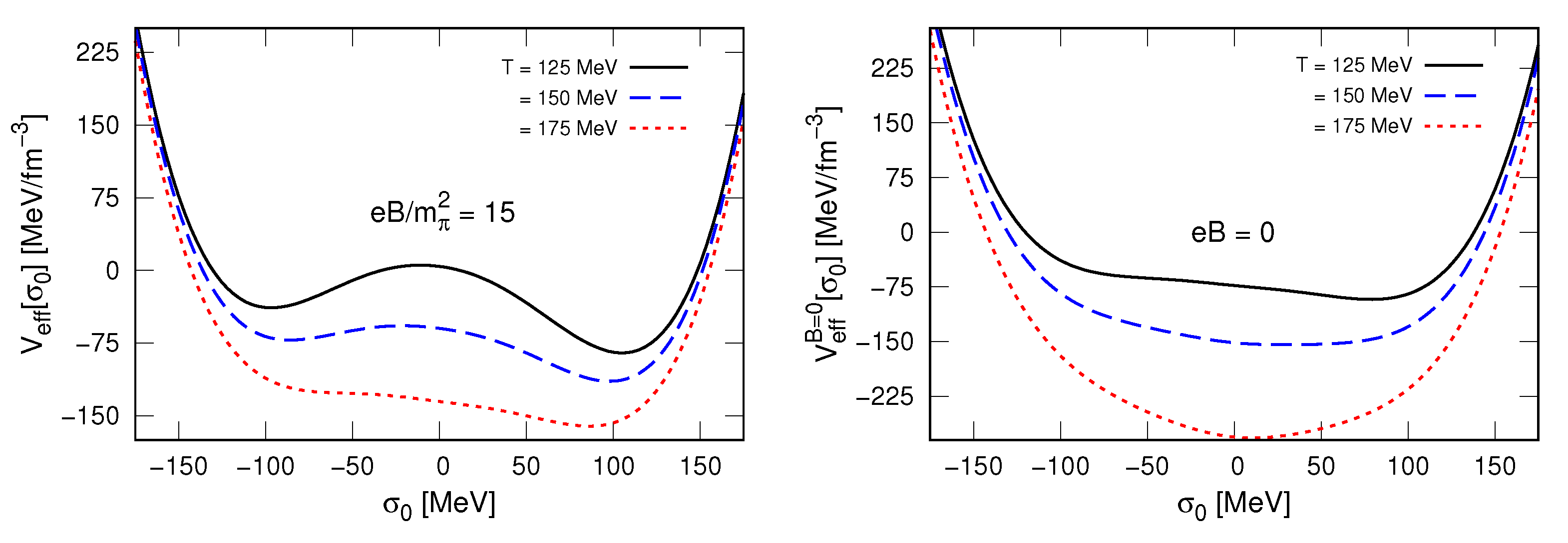
To orientate the discussion of results in the next section, we show in Figure 1 the effective potential $V_{\mathrm{eff}}\left[{\sigma }_0\right]$ for $B=15m_{\pi }^2$, Equation (69), and $B=0$, and temperatures around $T=150$ MeV. The effective potential for zero magnetic field, $V_{\mathrm{eff}}^{B=0}\left[{\sigma }_0\right]$, is given by [29]:

$$V_{\mathrm{eff}}^{B=0}\left[{\sigma }_0\right]=U\left[{\sigma }_0\right]-24T\int \frac{d^{3}p}{{\left(2\pi \right)}^3}ln\left[1+e^{-E\left(\mathit{p}\right)/T}\right],$$

(74)

where $E\left(\mathit{p}\right)=\sqrt{{\mathit{p}}^2+m_{\sigma }^2}$. The figure reveals that $|V_{\mathrm{eff}}|<|V_{\mathrm{eff}}^{B=0}|$ for $|{\sigma }_0|\le 100$ MeV, a feature due to a partial cancellation between ${\mathsf{\Omega }}^{BT}\left[{\sigma }_0\right]$ and ${\mathsf{\Omega }}^B\left[{\sigma }_0\right]$, with the latter being positive for those values of ${\sigma }_0$.

6. Dissipation and Noise, Short-Time Dynamics

We start examining the magnetic field impact on the damping coefficient $\eta$, the key quantity controlling the fluctuations in the $\sigma$ mean field dynamics. The zero magnetic field $\eta$ is given in References [24,29] for the zero mode only, $\mathit{p}=0$, for which $E_{\sigma }\approx \sqrt{{\mathit{p}}^2+m_{\sigma }^2}=m_{\sigma }$:

$${\eta }_0=g^2\frac{2N_c}{\pi }\left[1-2n_F(m_{\sigma }/2)\right]\frac{1}{m_{\sigma }^2}{\left(m_{\sigma }^2-4m_q^2\right)}^{3/2}.$$

(75)

Putting $E_{\sigma }=m_{\sigma }$ and ${\mathit{p}}_{\perp }=0$ in Equation (54), one obtains for the magnetic field dependent damping coefficient:

$${\eta }_B=g^2\frac{N_c}{4\pi }\left[1-2n_F(m_{\sigma }/2)\right]\left(eB\right)\frac{1}{m_{\sigma }^2}\sqrt{m_{\sigma }^2-4m_q^2}.$$

(76)

We obtain $m_{\sigma }$ from Equation (73). To have a real $\eta$, we must have $m_{\sigma }>2m_q$ in Equations (75) and (76), a constraint that reflects the kinematical limit for the $\sigma$ decay (at rest) into a quark-antiquark pair, $\sigma \to q\overline{q}$, the only source of dissipation in the model under the present approximations. We note that ${\eta }_0=0$ for $T<150$ MeV in this calculation due to the absence of pions; in the presence of pions, the decay $\sigma \to 2\pi$ leads to a nonzero $\eta$. We recall that our results are valid for strong magnetic fields only. Therefore, one cannot extrapolate our results to $B=0$; for weak magnetic fields, one needs to use a different representation for the magnetized quark propagator, as the LLL approximation is not valid in this case [58]. But, since weak fields (of strengths $\sqrt{eB}\ll {\mathsf{\Lambda }}_{\mathrm{QCD}}$) have little impact on chiral properties, we do not need alternative representations for the quark propagator.

Figure 2 displays the temperature dependence of the zero mode damping coefficient for $B=0$ and three $B\ne 0$ values. The magnetic field changes the qualitative temperature dependence of $\eta$ close to $T=150$ MeV. In a temperature quench scenario, $T\gg T_c^B\to T\ll T_c^B$, the nonzero value of ${\eta }_B$ for $T<T_c^B$ delays the start off of the condensate evolution after the quench. We extend the discussion on this issue at the end of this section, where we study explicit short-time solutions of the Langevin equation.

The magnetic field enters the expression for $\eta$, Equation (76), in two ways: through the multiplicative $eB$ term, and through the values of $m_{\sigma }$ and $m_q$. The latter dependence is subtle, B affects $m_{\sigma }$ and $m_q$ and thereby affects the inequality $m_{\sigma }>2m_q$. The magnetic field modifies not only the position of the minimum of $V_{\mathrm{eff}}$ (which determines $m_q$) but also its curvature around the minimum (which determines $m_{\sigma }$)—compare the $B\ne 0$ and $B=0$ effective potentials in Figure 1. To appreciate this B-dependence of $m_{\sigma }$ and $m_q$, we show in Figure 3 the temperature dependence of these masses for the values of B used in Figure 2. It is important to notice the different temperature dependence of $m_{\sigma }$ and $m_q$: the former increases faster as the temperature decreases. This faster increase of $m_{\sigma }$ explains the ${\eta }_B$ increase at low temperatures.

Continuing with the aim of gaining analytic understanding, we consider $\sigma$’s dynamics in a temperature quench scenario. Before continuing, we spell out the required simplifications here. We neglect expansion of the system. Expansion is perhaps the most relevant trait of a heavy-ion collision that needs to be taken into account when simulating a real laboratory event. But such a simulation is out of the scope of this work. We also assume a constant magnetic field in the course of the condensate evolution. As such, we do not consider the complex magnetohydrodynamics that governs the magnetic field in the medium expansion course. The magnetic field weakens as the system expands, but it also induces electric currents that can sustain a magnetic field of sizeable strength while the system exists [77,78,79]. This feature, to some extent, justifies the assumption of a constant field. Finally, we do no consider reheating, that is, energy transfer between the condensate and the background. Reheating changes the local temperature of the background and, as for zero magnetic fields, can effect the dynamics [30]. We reserve for a separate study the inclusion of the neglected effects.

In a quench scenario, a sudden drop in the temperature drives the system out of a high temperature phase, in which $\sigma \approx 0$, and forces the system to evolve to a lower temperature phase in which $\sigma \ne 0$. One gets insight on how a nonzero B impacts such a quench by examining the time scale controlling the short-time dynamics. That time scale, which we denote by ${\tau }_s$, determines how quickly the system leaves the initial state. It depends, of course, on $\eta$, and also on the nature of the lower temperature phase, which the magnetic field affects as well. This interplay between $\eta$ and the nature of the low temperature phase in a quench scenario is well known [18,19]. We take as lower temperature phase one around the $B=0$ pseudocritical temperature; that is, at $t=0$ the system is brought to one of the local maxima of the $V_{\mathrm{eff}}$ in Figure 1.

At short times, when $\sigma \approx 0$, one can linearize the Langevin equation, neglect the second-order time derivative, and solve the equation analytically. It is convenient [24] to rescale the fields by the volume $V=L^3$, namely $\overline{\sigma }=\sigma /L^3$ and ${\overline{\xi }}_{\sigma }={\xi }_{\sigma }/L^3$. The Langevin equation for $\overline{\sigma }$ can be written as:

$$\eta \left({\mathit{p}}_{\perp }\right)\frac{\partial \overline{\sigma }(t,{\mathit{p}}_{\perp })}{\partial t}-\left({\mu }^2-{\mathit{p}}_{\perp }^2\right)\overline{\sigma }(t,{\mathit{p}}_{\perp })+g{\rho }_s\left({\sigma }_0\right)-f_{\pi }{m}_{\pi }^2={\overline{\xi }}_{\sigma }(t,{\mathit{p}}_{\perp }),$$

(77)

where

$${\mu }^2=\lambda \left(f_{\pi }^2-\frac{m_{\pi }^2}{\lambda }\right),$$

(78)

and ${\xi }_{\sigma }$ has zero mean, ${\langle {\xi }_{\sigma }(t,{\mathit{p}}_{\perp })\rangle }_{\xi }=0$, and correlation

$${\langle {\xi }_{\sigma }(t,{\mathit{p}}_{\perp }){\xi }_{\sigma }(t^{\prime },{\mathit{p}}_{\perp }^{\prime })\rangle }_{\xi }={\left(2\pi \right)}^2\delta ({\mathit{p}}_{\perp }+{\mathit{p}}_{\perp }^{\prime })L\delta (t-t^{\prime })\overline{N}\left({\mathit{p}}_{\perp }\right),$$

(79)

where $\overline{N}\left({\mathit{p}}_{\perp }\right)=N\left({\mathit{p}}_{\perp }\right)/L^6$. We compute the equal-time correlation function (variance) of the field, ${\langle {\overline{\sigma }}^2(t,{\mathit{p}}_{\perp }^2)\rangle }_{\xi }$. Taking as initial condition $\overline{\sigma }(0,{\mathit{p}}_{\perp })=0$, one obtains:

$$\begin{array}{ccc}\hfill {\langle {\overline{\sigma }}^2(t,{\mathit{p}}_{\perp }^2)\rangle }_{\xi }& =& \frac{{\left[g{\rho }_s\left({\sigma }_0\right)-f_{\pi }{m}_{\pi }^2\right]}^2}{{({\mu }^2-{\mathit{p}}_{\perp })}^2}{\left(e^{\lambda \left({\mathit{p}}_{\perp }\right)t/{\tau }_s}-1\right)}^2\hfill \\ & & +\frac{E\left({\mathit{p}}_{\perp }\right)coth\left(E\left({\mathit{p}}_{\perp }\right)\right)}{L^3({\mu }^2-{\mathit{p}}_{\perp }^2)}\left(e^{2\lambda \left({\mathit{p}}_{\perp }\right)t/{\tau }_s}-1\right),\hfill \end{array}$$

(80)

where

$${\tau }_s=\frac{{\eta }_B}{{\mu }^2}\mathrm{and}\lambda \left({\mathit{p}}_{\perp }\right)=\frac{1-{\mathit{p}}_{\perp }^2/{\mu }^2}{\eta \left({\mathit{p}}_{\perp }\right)/{\eta }_B},$$

(81)

with ${\eta }_B$ given by Equation (76).

From the definition of $\lambda \left({\mathit{p}}_{\perp }\right)$ one sees that the exponentials in Equation (80) increase with time for long wavelength modes, ${\mathit{p}}_{\perp }^2<{\mu }^2$, and decrease for short wavelengths, ${\mathit{p}}_{\perp }^2>{\mu }^2$. That is, long wavelength modes explode at short times, akin to the familiar phenomenon of spinodal decomposition [18,19]. We recall that the quench we are considering brings the system to one of the local maxima of the effective potential $V_{\mathrm{eff}}$ in Figure 1; there are no barriers to overcome. The explosion is controlled by the time scale ${\tau }_s$, which depends on $\eta$ (fluctuations) and ${\mu }^2$ (state). The first term in Equation (80) exposes the role played by the low temperature phase; it comes from $\delta V_{\mathrm{eff}}\left[\sigma \right]/\delta \sigma$. Notice that for small $\sigma$, that term is nothing else $\delta V_{\mathrm{eff}}\left[\sigma \right]/\delta \sigma =0$: $(g{\rho }_s-f_{\pi }{m}_{\pi }^2)/{\mu }^2\equiv {\sigma }_s^2$, where ${\sigma }_s$ stands for small $\sigma$. The second term comes from the noise source.

We present results for the (square root of the) equal-time correlation function for two values of ${\mathit{p}}_{\perp }$; the zero mode ${\mathit{p}}_{\perp }=0$, and a thermal average value ${\langle p_{\perp }\rangle }_{\mathrm{th}.}=\sqrt{{\langle {\mathit{p}}_{\perp }^2\rangle }_{\mathrm{th}.}}$, where ${\langle {\mathit{p}}_{\perp }^2\rangle }_{\mathrm{th}.}$ is the average:

$${\langle {\mathit{p}}_{\perp }^2\rangle }_{\mathrm{th}.}=\frac{\int d^2{p}_{\perp }{p}_{\perp }^2{n}_B\left({\mathit{p}}_{\perp }\right)}{\int d^2{p}_{\perp }{n}_B\left(p_{\perp }\right)},\mathrm{where}{n}_B\left(p\right)=\frac{1}{e^{E_{\sigma }\left(p\right)/T}-1},$$

(82)

with $E_{\sigma }\left(p\right)=\sqrt{p^2+m_{\sigma }^2}$. We take a volume of dimension $L^3={\left(10\mathrm{fm}\right)}^3$. Figure 4 shows results for $\langle \overline{\sigma }\rangle (t,{\mathit{p}}_{\perp })/{\sigma }_s$, where we defined $\langle \overline{\sigma }\rangle (t,{\mathit{p}}_{\perp })=\sqrt{{\langle {\overline{\sigma }}^2(t,{\mathit{p}}_{\perp })\rangle }_{\xi }}$. The zero mode’s fast exponential growth stands out in the two panels of the figure. The magnetic field impact on the short-time growth also stands out, notably the explosion delay alluded to previously. Since our calculation does not take into account expansion of the system, it is difficult to assess the phenomenological impact of such a delay, for example, on the QGP disassemble into hadrons. However, the delay does not seem irrelevant in this respect, as it can reach $1\mathrm{fm}$ (right panel of Figure 4), being of the order of 10% of the total time the QGP takes to disassemble into hadrons. We recall that the latter is on the average of the order of $10\mathrm{fm}$, time over which the temperature varies between $T_{\mathrm{ch}}\sim 150\mathrm{MeV}$ and $T_{\mathrm{K}}\sim 100\mathrm{MeV}$ [80,81]. Here, $T_{\mathrm{ch}}$ and $T_{\mathrm{K}}$ are respectively the chemical and kinetic freeze out temperatures; the former signals the end of inelastic collisions and fixes the observed hadron abundances and the latter signals the end of elastic hadron collisions and leads to the disassemble of the system into hadrons. Given that a magnetic field also affects hadron masses, there seems to be room for optimism for a possible experimental signal in hadron emission spectra from noncentral collisions. Certainly these results warrant further studies.

Will pions change qualitatively the overall picture? Probably not. For $B=0$, pions have a significant effect on the $\sigma$ dynamics only close to the first-order transition of the LSMq [82]. The results we have shown here refer to temperatures away from the first order transition temperature, which we recall, $T\ge 180$ MeV. Moreover, results from lattice QCD [83] and phenomenological models [58,84,85] predict that a background magnetic field leaves unchanged the ${\pi }^0$ mass and increases the ${\pi }^{\pm }$ masses, as expected on general grounds, features that will not change the results of Reference [82]. An instance where pions will change quantitatively our results is in the value of $\eta$: pions bring further dissipation with the $\sigma \to 2\pi$ channel, which implies a positive contribution to ${\tau }_s$, that is, the delay increases. However, the question will be answered only with a detailed calculation.

7. Conclusions and Perspectives

We studied the impact of a strong magnetic field on the chiral quark condensate dynamics. We built on the semiclassical framework developed for zero magnetic field developed in Reference [29]. That framework bases the dynamics on a mean field Langevin equation derived from a microscopic chiral quark model. We extended that Langevin equation to include the effects of a magnetic field. The Langevin equation we derived features damping and noise modified by the magnetic field. Damping and noise reflect the condensate’s interactions with an effective magnetized quark background in local thermal equilibrium. The background results from integrating out quarks from a mean-field effective action defined by the linear sigma model. To integrate out quarks, we used the closed time path formalism of nonequilibrium quantum field theory. We obtained numerical results using values of magnetic field strengths and space-time scales related to high-energy heavy-ion collision experiments. We presented results for the short-time condensate dynamics under temperature quenches. The quenches we used were from a high temperature, for which the condensate is zero, to lower temperatures close to the zero magnetic field crossover temperature, $T\sim 150$ MeV. The results we showed revealed that the magnetic field changes the dissipation pattern as compared to the zero magnetic field case, retarding condensate’s short-time evolution substantially, a feature that can impact hadron formation at the QCD transition.

Our study was a first incursion into a complex many-body problem. Our primary aim in this study was to get insight into how a strong magnetic field affects condensate dynamics. We simplified the analysis, and sought an analytical understanding whenever possible. We also omitted physical effects peculiar to a heavy-ion collision. As such, before one can draw conclusions on phenomenological consequences in a realist heavy-ion setting, one needs to extend the theoretical framework to include the omitted features. These include pions, expansion, reheating, magnetohydrodynamics modes, and coupling to other order parameters. As in the case of zero magnetic field [29], the formalism developed here is flexible enough to tackle the more complex problem. Another extension of our study is to incorporate a confinement mechanism. A possibility is to couple a color dielectric field to the chiral $\sigma$ and $\mathit{\pi }$ fields of the LSMq, a possibility very much explored in the context of bag and soliton models [86]. Such models can be extended to include explicit gluon degrees of freedom to realize dynamical chiral symmetry breaking and describe asymptotic freedom [87,88].

The framework developed in this paper can be adapted to study magnetic field effects on the QCD phase transition in the early universe and in the interior of magnetized compact stars (magnetars). Several mechanisms of strong magnetic field generation in the early universe have been suggested [7,8]; a very recent, connected with the QCD phase transition, involves the collapse of domain walls related to the confinement order parameter [89]. A marked difference between the early universe and heavy-ion collision settings concerns the rate of change of the temperature $dlnT/dt$ during expansion of the system. In the early universe, this rate is given by Hubble constant $H\sim {10}^{-18}{s}^{-1}$, which is much slower than that in a heavy-ion collision. Therefore, the primordial chiral condensate evolves in a slowly changing effective potential as the system expands. Such an evolution characterizes an annealing scenario for the phase change, rather than of a quench, but it can be studied equally well with the Langevin equation framework of the present paper [90]. Regarding magnetars, the inner-core magnetic field can reach strengths varying between $eB\simeq m_{\pi }^2$ and $eB\simeq 50m_{\pi }^2$ [91]. In this setting, the temperatures are very low, lower than 50 MeV, and the phase conversion is driven by high baryon density. An issue of interest relates to the time scales associated with the phase conversion during the early stages of the magnetar formation after a core-collapsing supernova process. In this case, the formalism used in this paper needs to be extended to nonzero baryon density [92].

References

- D’Elia, M. Lattice QCD Simulations in External Background Fields. Lect. Notes Phys. 2013, 871, 181–208. [Google Scholar] [CrossRef] [Green Version]
- Endrödi, G. QCD in magnetic fields: From Hofstadter’s butterfly to the phase diagram. PoS 2014, LATTICE2014, 018. [Google Scholar] [CrossRef] [Green Version]
- Ding, H.T.; Li, S.T.; Shi, Q.; Tomiya, A.; Wang, X.D.; Zhang, Y. QCD phase structure in strong magnetic fields. In Proceedings of the Criticality in QCD and the Hadron Resonance Gas, Wroclaw, Poland, 29–31 July 2020. [Google Scholar]
- Aoki, Y.; Endrodi, G.; Fodor, Z.; Katz, S.; Szabo, K. The Order of the quantum chromodynamics transition predicted by the standard model of particle physics. Nature 2006, 443, 675–678. [Google Scholar] [CrossRef] [PubMed] [Green Version]
- Wilczek, F. The Lightness of Being: Mass, Ether, and the Unification of Forces; Basic Books: New York, NY, USA, 2008. [Google Scholar]
- Roberts, C.D. Empirical Consequences of Emergent Mass. Symmetry 2020, 12, 1468. [Google Scholar] [CrossRef]
- Vachaspati, T. Magnetic fields from cosmological phase transitions. Phys. Lett. B 1991, 265, 258–261. [Google Scholar] [CrossRef]
- Grasso, D.; Rubinstein, H.R. Magnetic fields in the early universe. Phys. Rept. 2001, 348, 163–266. [Google Scholar] [CrossRef] [Green Version]
- Kouveliotou, C.; Dieters, S.; Strohmayer, T.; van Paradijs, J.; Fishman, G.J.; Meegan, C.A.; Hurley, K.; Kommers, J.; Smith, I.; Frail, D.; et al. An X-ray pulsar with a superstrong magnetic field in the soft gamma-ray repeater SGR 1806-20. Nature 1998, 393, 235–237. [Google Scholar] [CrossRef]
- Duncan, R.C.; Thompson, C. Formation of very strongly magnetized neutron stars-implications for gamma-ray bursts. Astrophys. J. Lett. 1992, 392, L9. [Google Scholar] [CrossRef]
- Rafelski, J.; Muller, B. Magnetic Splitting of Quasimolecular Electronic States in Strong Fields. Phys. Rev. Lett. 1976, 36, 517. [Google Scholar] [CrossRef]
- Kharzeev, D.E.; McLerran, L.D.; Warringa, H.J. The Effects of topological charge change in heavy ion collisions: ’Event by event P and CP violation’. Nucl. Phys. A 2008, 803, 227–253. [Google Scholar] [CrossRef] [Green Version]
- Skokov, V.; Illarionov, A.; Toneev, V. Estimate of the magnetic field strength in heavy-ion collisions. Int. J. Mod. Phys. A 2009, 24, 5925–5932. [Google Scholar] [CrossRef] [Green Version]
- Jacak, B.V.; Muller, B. The exploration of hot nuclear matter. Science 2012, 337, 310–314. [Google Scholar] [CrossRef] [PubMed] [Green Version]
- Shuryak, E. Strongly coupled quark-gluon plasma in heavy ion collisions. Rev. Mod. Phys. 2017, 89, 035001. [Google Scholar] [CrossRef] [Green Version]
- Pasechnik, R.; Šumbera, M. Phenomenological Review on Quark–Gluon Plasma: Concepts vs. Observations. Universe 2017, 3, 7. [Google Scholar] [CrossRef] [Green Version]
- Braun-Munzinger, P.; Koch, V.; Schäfer, T.; Stachel, J. Properties of hot and dense matter from relativistic heavy ion collisions. Phys. Rept. 2016, 621, 76–126. [Google Scholar] [CrossRef] [Green Version]
- Goldenfeld, N. Lectures on Phase Transitions and the Renormalization Group; Perseus Books: Reading, MA, USA, 1992. [Google Scholar]
- Onuki, A. Phase Transition Dynamics; Cambridge University Press: Cambridge, UK, 2002. [Google Scholar]
- Rajagopal, K.; Wilczek, F. Emergence of coherent long wavelength oscillations after a quench: Application to QCD. Nucl. Phys. B 1993, 404, 577–589. [Google Scholar] [CrossRef] [Green Version]
- Bedaque, P.F.; Das, A.K. Out-of-equilibrium phase transitions and a toy model for disoriented chiral condensates. Mod. Phys. Lett. A 1993, 8, 3151–3164. [Google Scholar] [CrossRef] [Green Version]
- Greiner, C.; Muller, B. Classical fields near thermal equilibrium. Phys. Rev. D 1997, 55, 1026–1046. [Google Scholar] [CrossRef] [Green Version]
- Biro, T.S.; Greiner, C. Dissipation and fluctuation at the chiral phase transition. Phys. Rev. Lett. 1997, 79, 3138–3141. [Google Scholar] [CrossRef] [Green Version]
- Rischke, D.H. Forming disoriented chiral condensates through fluctuations. Phys. Rev. C 1998, 58, 2331–2357. [Google Scholar] [CrossRef] [Green Version]
- Xu, Z.; Greiner, C. Stochastic treatment of disoriented chiral condensates within a Langevin description. Phys. Rev. D 2000, 62, 036012. [Google Scholar] [CrossRef] [Green Version]
- Fraga, E.S.; Krein, G. Can dissipation prevent explosive decomposition in high-energy heavy ion collisions? Phys. Lett. B 2005, 614, 181–186. [Google Scholar] [CrossRef] [Green Version]
- Boyanovsky, D.; de Vega, H.J.; Schwarz, D.J. Phase transitions in the early and the present universe. Ann. Rev. Nucl. Part. Sci. 2006, 56, 441–500. [Google Scholar] [CrossRef] [Green Version]
- Farias, R.; Cassol-Seewald, N.; Krein, G.; Ramos, R. Nonequilibrium dynamics of quantum fields. Nucl. Phys. A 2007, 782, 33–36. [Google Scholar] [CrossRef] [Green Version]
- Nahrgang, M.; Leupold, S.; Herold, C.; Bleicher, M. Nonequilibrium chiral fluid dynamics including dissipation and noise. Phys. Rev. C 2011, 84, 024912. [Google Scholar] [CrossRef] [Green Version]
- Nahrgang, M.; Leupold, S.; Bleicher, M. Equilibration and relaxation times at the chiral phase transition including reheating. Phys. Lett. B 2012, 711, 109–116. [Google Scholar] [CrossRef] [Green Version]
- Nahrgang, M.; Herold, C.; Leupold, S.; Mishustin, I.; Bleicher, M. The impact of dissipation and noise on fluctuations in chiral fluid dynamics. J. Phys. G 2013, 40, 055108. [Google Scholar] [CrossRef]
- Singh, A.; Puri, S.; Mishra, H. Domain growth in chiral phase transitions. Nucl. Phys. A 2011, 864, 176–202. [Google Scholar] [CrossRef] [Green Version]
- Krein, G. Noise and ultraviolet divergences in the dynamics of the chiral condensate in QCD. J. Phys. Conf. Ser. 2012, 378, 012032. [Google Scholar] [CrossRef] [Green Version]
- Cassol-Seewald, N.; Farias, R.S.; Krein, G.; Marques de Carvalho, R. Noise and ultraviolet divergences in simulations of Ginzburg-Landau-Langevin type of equations. Int. J. Mod. Phys. C 2012, 23, 1240016. [Google Scholar] [CrossRef]
- Singh, A.; Puri, S.; Mishra, H. Domain growth in chiral phase transitions: Role of inertial dynamics. Nucl. Phys. A 2013, 908, 12–28. [Google Scholar] [CrossRef] [Green Version]
- Herold, C.; Nahrgang, M.; Mishustin, I.; Bleicher, M. Chiral fluid dynamics with explicit propagation of the Polyakov loop. Phys. Rev. C 2013, 87, 014907. [Google Scholar] [CrossRef]
- Singh, A.; Puri, S.; Mishra, H. Kinetics of phase transitions in quark matter. EPL 2013, 102, 52001. [Google Scholar] [CrossRef] [Green Version]
- Bluhm, M.; Jiang, Y.; Nahrgang, M.; Pawlowski, J.; Rennecke, F.; Wink, N. Time-evolution of fluctuations as signal of the phase transition dynamics in a QCD-assisted transport approach. Nucl. Phys. A 2019, 982, 871–874. [Google Scholar] [CrossRef]
- Wu, S.; Wu, Z.; Song, H. Universal scaling of the σ field and net-protons from Langevin dynamics of model A. Phys. Rev. C 2019, 99, 064902. [Google Scholar] [CrossRef] [Green Version]
- Calzetta, E.A.; Hu, B.L.B. Nonequilibrium Quantum Field Theory, Cambridge Monographs on Mathematical Physics; Cambridge University Press: Cambridge, UK, 2008. [Google Scholar] [CrossRef]
- Bellac, M.L. Thermal Field Theory, Cambridge Monographs on Mathematical Physics; Cambridge University Press: Cambridge, UK, 2011. [Google Scholar] [CrossRef]
- Gell-Mann, M.; Levy, M. The axial vector current in beta decay. Nuovo Cim. 1960, 16, 705. [Google Scholar] [CrossRef]
- Fraga, E.S.; Mizher, A.J. Chiral transition in a strong magnetic background. Phys. Rev. D 2008, 78, 025016. [Google Scholar] [CrossRef] [Green Version]
- Ayala, A.; Bashir, A.; Raya, A.; Sanchez, A. Chiral phase transition in relativistic heavy-ion collisions with weak magnetic fields: Ring diagrams in the linear sigma model. Phys. Rev. D 2009, 80, 036005. [Google Scholar] [CrossRef] [Green Version]
- Frasca, M.; Ruggieri, M. Magnetic Susceptibility of the Quark Condensate and Polarization from Chiral Models. Phys. Rev. D 2011, 83, 094024. [Google Scholar] [CrossRef] [Green Version]
- Andersen, J.O.; Khan, R. Chiral transition in a magnetic field and at finite baryon density. Phys. Rev. D 2012, 85, 065026. [Google Scholar] [CrossRef] [Green Version]
- Andersen, J.O.; Tranberg, A. The Chiral transition in a magnetic background: Finite density effects and the functional renormalization group. JHEP 2012, 08, 002. [Google Scholar] [CrossRef] [Green Version]
- Ruggieri, M.; Tachibana, M.; Greco, V. Renormalized vs Nonrenormalized Chiral Transition in a Magnetic Background. JHEP 2013, 07, 165. [Google Scholar] [CrossRef] [Green Version]
- Fraga, E.S.; Mintz, B.W.; Schaffner-Bielich, J. A search for inverse magnetic catalysis in thermal quark-meson models. Phys. Lett. B 2014, 731, 154–158. [Google Scholar] [CrossRef] [Green Version]
- Kamikado, K.; Kanazawa, T. Chiral dynamics in a magnetic field from the functional renormalization group. JHEP 2014, 03, 009. [Google Scholar] [CrossRef] [Green Version]
- Ruggieri, M.; Oliva, L.; Castorina, P.; Gatto, R.; Greco, V. Critical Endpoint and Inverse Magnetic Catalysis for Finite Temperature and Density Quark Matter in a Magnetic Background. Phys. Lett. B 2014, 734, 255–260. [Google Scholar] [CrossRef]
- Ayala, A.; Hernández, L.A.; Mizher, A.J.; Rojas, J.C.; Villavicencio, C. Chiral transition with magnetic fields. Phys. Rev. D 2014, 89, 116017. [Google Scholar] [CrossRef] [Green Version]
- Ayala, A.; Loewe, M.; Zamora, R. Inverse magnetic catalysis in the linear sigma model with quarks. Phys. Rev. D 2015, 91, 016002. [Google Scholar] [CrossRef] [Green Version]
- Andersen, J.O.; Naylor, W.R.; Tranberg, A. Inverse magnetic catalysis and regularization in the quark-meson model. JHEP 2015, 2, 042. [Google Scholar] [CrossRef] [Green Version]
- Ayala, A.; Dominguez, C.A.; Hernandez, L.A.; Loewe, M.; Zamora, R. Magnetized effective QCD phase diagram. Phys. Rev. D 2015, 92, 096011. [Google Scholar] [CrossRef] [Green Version]
- Gatto, R.; Ruggieri, M. Quark Matter in a Strong Magnetic Background. Lect. Notes Phys. 2013, 871, 87–119. [Google Scholar] [CrossRef] [Green Version]
- Ayala, A.; Loewe, M.; Villavicencio, C.; Zamora, R. On the magnetic catalysis and inverse catalysis of phase transitions in the linear sigma model. Nucl. Part. Phys. Proc. 2015, 258–259, 209–212. [Google Scholar] [CrossRef] [Green Version]
- Miransky, V.A.; Shovkovy, I.A. Quantum field theory in a magnetic field: From quantum chromodynamics to graphene and Dirac semimetals. Phys. Rept. 2015, 576, 1–209. [Google Scholar] [CrossRef] [Green Version]
- Andersen, J.O.; Naylor, W.R.; Tranberg, A. Phase diagram of QCD in a magnetic field: A review. Rev. Mod. Phys. 2016, 88, 025001. [Google Scholar] [CrossRef]
- Bjorken, J.D.; Drell, S.D. Relativistic Quantum Fields; McGraw-Hill: New York, NY, USA, 1965. [Google Scholar]
- Koch, V. Aspects of chiral symmetry. Int. J. Mod. Phys. E 1997, 6, 203–250. [Google Scholar] [CrossRef] [Green Version]
- Kamenev, A. Field Theory of Non-Equilibrium Systems; Cambridge University Press: Cambridge, UK, 2011. [Google Scholar]
- Martin, P.; Siggia, E.; Rose, H. Statistical Dynamics of Classical Systems. Phys. Rev. A 1973, 8, 423–437. [Google Scholar] [CrossRef]
- Feynman, R.; Vernon, F.L.J. The Theory of a general quantum system interacting with a linear dissipative system. Ann. Phys. 1963, 24, 118–173. [Google Scholar] [CrossRef] [Green Version]
- Loewe, M.; Rojas, J. Thermal effects and the effective action of quantum electrodynamics. Phys. Rev. D 1992, 46, 2689–2694. [Google Scholar] [CrossRef] [PubMed]
- Elmfors, P.; Persson, D.; Skagerstam, B.S. QED effective action at finite temperature and density. Phys. Rev. Lett. 1993, 71, 480–483. [Google Scholar] [CrossRef] [Green Version]
- Hasan, M.; Chatterjee, B.; Patra, B.K. Heavy Quark Potential in a static and strong homogeneous magnetic field. Eur. Phys. J. C 2017, 77, 767. [Google Scholar] [CrossRef]
- Rath, S.; Patra, B.K. One-loop QCD thermodynamics in a strong homogeneous and static magnetic field. JHEP 2017, 12, 098. [Google Scholar] [CrossRef] [Green Version]
- Schwinger, J.S. On gauge invariance and vacuum polarization. Phys. Rev. 1951, 82, 664–679. [Google Scholar] [CrossRef]
- Das, A.; Deshamukhya, A.; Kalauni, P.; Panda, S. Bogoliubov transformation and the thermal operator representation in the real time formalism. Phys. Rev. D 2018, 97, 045015. [Google Scholar] [CrossRef] [Green Version]
- Menezes, D.P.; Benghi Pinto, M.; Avancini, S.S.; Perez Martinez, A.; Providencia, C. Quark matter under strong magnetic fields in the Nambu-Jona-Lasinio Model. Phys. Rev. C 2009, 79, 035807. [Google Scholar] [CrossRef] [Green Version]
- Farias, R.L.S.; Gomes, K.P.; Krein, G.I.; Pinto, M.B. Importance of asymptotic freedom for the pseudocritical temperature in magnetized quark matter. Phys. Rev. C 2014, 90, 025203. [Google Scholar] [CrossRef] [Green Version]
- Cassol-Seewald, N.; Copetti, M.; Krein, G. Numerical approximation of the Ginzburg–Landau equation with memory effects in the dynamics of phase transitions. Comput. Phys. Commun. 2008, 179, 297–309. [Google Scholar] [CrossRef]
- Ebert, D.; Klimenko, K.G.; Vdovichenko, M.A.; Vshivtsev, A.S. Magnetic oscillations in dense cold quark matter with four fermion interactions. Phys. Rev. D 2000, 61, 025005. [Google Scholar] [CrossRef] [Green Version]
- Bali, G.; Bruckmann, F.; Endrodi, G.; Fodor, Z.; Katz, S.; Krieg, S.; Schafer, A.; Szabo, K. The QCD phase diagram for external magnetic fields. JHEP 2012, 02, 044. [Google Scholar] [CrossRef] [Green Version]
- Bali, G.; Bruckmann, F.; Endrodi, G.; Fodor, Z.; Katz, S.; Schafer, A. QCD quark condensate in external magnetic fields. Phys. Rev. D 2012, 86, 071502. [Google Scholar] [CrossRef] [Green Version]
- Tuchin, K. Time and space dependence of the electromagnetic field in relativistic heavy-ion collisions. Phys. Rev. C 2013, 88, 024911. [Google Scholar] [CrossRef] [Green Version]
- Gursoy, U.; Kharzeev, D.; Rajagopal, K. Magnetohydrodynamics, charged currents and directed flow in heavy ion collisions. Phys. Rev. C 2014, 89, 054905. [Google Scholar] [CrossRef] [Green Version]
- Tuchin, K. Initial value problem for magnetic fields in heavy ion collisions. Phys. Rev. C 2016, 93, 014905. [Google Scholar] [CrossRef]
- Busza, W.; Rajagopal, K.; van der Schee, W. Heavy Ion Collisions: The Big Picture, and the Big Questions. Ann. Rev. Nucl. Part. Sci. 2018, 68, 339–376. [Google Scholar] [CrossRef] [Green Version]
- Chatterjee, S.; Das, S.; Kumar, L.; Mishra, D.; Mohanty, B.; Sahoo, R.; Sharma, N. Freeze-Out Parameters in Heavy-Ion Collisions at AGS, SPS, RHIC, and LHC Energies. Adv. High Energy Phys. 2015, 2015, 349013. [Google Scholar] [CrossRef]
- Weissenborn-Bresch, S.A. On the Impact of Pion Fluctuations on the Dynamics of the Order Parameter at the Chiral Phase Transition; Ruperto-Carola-University of Heidelberg: Heidelberg, Germany, 2016. [Google Scholar] [CrossRef]
- Bali, G.S.; Brandt, B.B.; Endrődi, G.; Gläßle, B. Meson masses in electromagnetic fields with Wilson fermions. Phys. Rev. D 2018, 97, 034505. [Google Scholar] [CrossRef] [Green Version]
- Andersen, J.O. Chiral perturbation theory in a magnetic background-finite-temperature effects. JHEP 2012, 10, 005. [Google Scholar] [CrossRef] [Green Version]
- Dumm, D.G.; Carlomagno, J.P.; Scoccola, N.N. Strong-interaction matter under extreme conditions from chiral quark models with nonlocal separable interactions. Symmetry 2021, 13, 121. [Google Scholar] [CrossRef]
- Birse, M.C. Soliton models for nuclear physics. Prog. Part. Nucl. Phys. 1990, 25, 1–80. [Google Scholar] [CrossRef]
- Krein, G.; Tang, P.; Wilets, L.; Williams, A.G. Confinement, Chiral Symmetry Breaking and the Pion in a Chromodielectric Model of Quantum Chromodynamics. Phys. Lett. B 1988, 212, 362–368. [Google Scholar] [CrossRef]
- Krein, G.; Tang, P.; Wilets, L.; Williams, A.G. The Chromodielectric model: Confinement, chiral symmetry breaking, and the pion. Nucl. Phys. A 1991, 523, 548–562. [Google Scholar] [CrossRef]
- Atreya, A.; Sanyal, S. Generation of magnetic fields near QCD Transition by collapsing Z(3) domains. Eur. Phys. J. C 2018, 78, 1027. [Google Scholar] [CrossRef]
- Gavin, S.; Muller, B. Larger domains of disoriented chiral condensate through annealing. Phys. Lett. B 1994, 329, 486–492. [Google Scholar] [CrossRef] [Green Version]
- Ferrer, E.J.; Hackebill, A. Equation of State of a Magnetized Dense Neutron System. Universe 2019, 5, 104. [Google Scholar] [CrossRef] [Green Version]
- Kroff, D.; Fraga, E.S. Nucleating quark droplets in the core of magnetars. Phys. Rev. D 2015, 91, 025017. [Google Scholar] [CrossRef] [Green Version]
Figure 1.
Effective potential for temperatures close to the crossover temperature.
Figure 2.
Temperature and magnetic field dependence of the zero mode damping coefficient. Temperature range chosen to include the pseudocritical temperature, MeV.
Figure 3.
Temperature and magnetic field dependence of the and quark masses.
Figure 4.
Square root of the equal-time correlation function, normalized to —see text for definitions. Notice the different vertical axes ranges in two panels. There is no dashed-red curve for in the left panel because is zero for and MeV (see Figure 2).
Publisher’s Note: MDPI stays neutral with regard to jurisdictional claims in published maps and institutional affiliations. |
© 2021 by the authors. Licensee MDPI, Basel, Switzerland. This article is an open access article distributed under the terms and conditions of the Creative Commons Attribution (CC BY) license (https://creativecommons.org/licenses/by/4.0/).
Share and Cite
MDPI and ACS Style
Krein, G.; Miller, C. Nonequilibrium Dynamics of the Chiral Quark Condensate under a Strong Magnetic Field. Symmetry 2021, 13, 551. https://0-doi-org.brum.beds.ac.uk/10.3390/sym13040551
AMA Style
Krein G, Miller C. Nonequilibrium Dynamics of the Chiral Quark Condensate under a Strong Magnetic Field. Symmetry. 2021; 13(4):551. https://0-doi-org.brum.beds.ac.uk/10.3390/sym13040551
Chicago/Turabian StyleKrein, Gastão, and Carlisson Miller. 2021. "Nonequilibrium Dynamics of the Chiral Quark Condensate under a Strong Magnetic Field" Symmetry 13, no. 4: 551. https://0-doi-org.brum.beds.ac.uk/10.3390/sym13040551
Note that from the first issue of 2016, this journal uses article numbers instead of page numbers. See further details here.