
Vibration Properties of a Concrete Structure with Symmetries Used in Civil Engineering


1
Department of Mechanical Engineering, Transilvania University of Brasov, B-dul Eroilor 20, 500036 Brasov, Romania
2
Romanian Academy of Technical Sciences, B-dul Dacia 26, 030167 Bucharest, Romania
3
Department of Mathematics and Computer Science, Transilvania University of Brasov, B-dul Eroilor 29, 500036 Brasov, Romania
4
Department of Civil Engineering, Transilvania University of Brasov, 500036 Brasov, Romania
*
Author to whom correspondence should be addressed.
Symmetry 2021, 13(4), 656; https://0-doi-org.brum.beds.ac.uk/10.3390/sym13040656
Submission received: 22 March 2021
/
Revised: 7 April 2021
/
Accepted: 9 April 2021
/
Published: 12 April 2021
(This article belongs to the Special Issue Symmetry in Modeling and Analysis of Dynamic Systems)
Abstract
:The paper aims to study a concrete structure, currently used in civil engineering, which has certain symmetries. This type of problem is common in engineering practice, especially in civil engineering. There are many reasons why structures with identical elements or certain symmetries are used in industry, related to economic considerations, shortening the design time, for constructive, simplicity, cost or logistical reasons. There are many reasons why the presence of symmetries has benefits for designers, builders, and beneficiaries. In the end, the result of these benefits materializes through short execution times and reduced costs. The paper studies the eigenvalue and eigenmode properties of vibration for components of the constructions’ structure, often encountered in current practice. The identification of such properties allows the simplification and easing of the effort necessary for the dynamic analysis of such a structure.
1. Introduction
Frequently encountered in the design and construction of structures used in civil engineering, symmetries allow, in many cases, the simplification of calculations and dynamic analysis of such a structure. The direct consequence would be the shortening of the design and execution time and, of course, the decrease of the costs generated by these stages. The smaller information provided by a repetitive or symmetrical structure can help ease the computational effort. In the case of a static calculation, methods of approaching this problem are presented in the Strength of Materials courses. In the dynamic case, considering the elastic elements and studying the vibrations, although certain properties have long been observed [1], a systematic study of the problem has not yet been done. A case in which the symmetries introduced by two identical motors and their effect on vibrations were considered was studied [2]. The use of identical systems was applied to the design of a centrifugal pendulum vibration absorber system [3]. Circular symmetry and its induced properties have been reported previously [4,5]. Other particular cases have been studied [6] using a finite difference method and [7] for continuous systems. In the following, we will study the case of a mechanical system consisting of four trusses, two of which are identical. The transverse and torsional vibrations of such a system that are strongly coupled for the chosen case will be studied.
In the field of engineering, not only in civil engineering, but also in other fields such as the machine or machinery manufacturing industry, the automotive industry, and the aerospace industry, there are products, parts of products, machines, and components that contain identical, repetitive elements, which have, in their composition, parts that show symmetries of different types.
Until now, symmetries in Mechanics have been studied mainly from the point of view of the mathematics involved [8], as they have effects in writing equations of motion [9], but their applications in practice are little studied [10]. In January 2018, a special issue of the Symmetry review dedicated to applications in Structural Mechanics (Civil Engineering and Symmetry-2018, ISSN 2073-8994, [11]) was launched. The course Similarity, Symmetry and Group Theoretical Methods in Mechanics was organized at the Center for Solid Mechanics-CISM from UDINE (see ref. [12]).
The use of substructures in the design of the aeronautical industry is a relatively common procedure used to reduce working time. Finite element models of different parts are condensed into substructures. Obviously a substructure contains less degree of freedom (DOF) than the entire structure and it is easier to model it. Likewise, for identical parts that are found in the construction and design of aeronautical panels, if the substructure has been generated for one part, the generation of the whole assembly becomes easier to do. A method reduces the size of the model, useful in the design stage and in the manufacture of the entire structure. The accuracy of the finite element analysis performed is maintained. An illustration of this method is presented in a previous work [13].
The modeling of mechanical systems with repetitive or identical parts leads, finally, to systems of differential equations that describe the answer of such systems, which have, in their component, strings of identical terms. This feature leads to simpler methods of solving these systems of differential equations. Such an issue is addressed in studies [14,15].
The vast majority of buildings, works of art, halls, and in general, the constructions, have identical parts and have symmetries. It is a situation that has existed since the beginning of the first constructions made by man (antiquity) and the reasons are of several kinds as an easier, faster design, then a cheaper realization and, less important for engineers but important for beneficiaries, for aesthetic reasons. The structures have in their composition repetitive elements or present different forms of symmetry. These properties can be used successfully to facilitate static and dynamic analysis.
Group theory has been used extensively to study various phenomena in physics and chemistry, such as quantum mechanics, crystallography, and molecular structure. However, this theory can find a fertile field of application in engineering. This allows simplifying the analysis of systems that have certain symmetries or identical parts. In this way, it was efficient in the study of vibrations or the dynamic or kinematic analysis of mechanical systems. The use of group theory in engineering was analyzed [16,17]. Different aspects of the use of symmetry in engineering are presented in other papers. In a research [18], the influence of the symmetry of boundary condition in the description of the models was studied. Some theoretical basis and an attempt to classify the symmetries that occur in structures were presented [19] and application of the symmetry in engineering structures were presented [20,21].
In recent years, new and interesting methods of studying this type of problem have been studied by researchers [22,23] and new ways to deal with such problems were reported [24,25].
However, there are still many situations that can be studied and, therefore, the present paper aims to complete the cases studied and to offer proposals for the application of these properties that could help a design engineer to ease his effort.
2. Model and Free Vibration Response
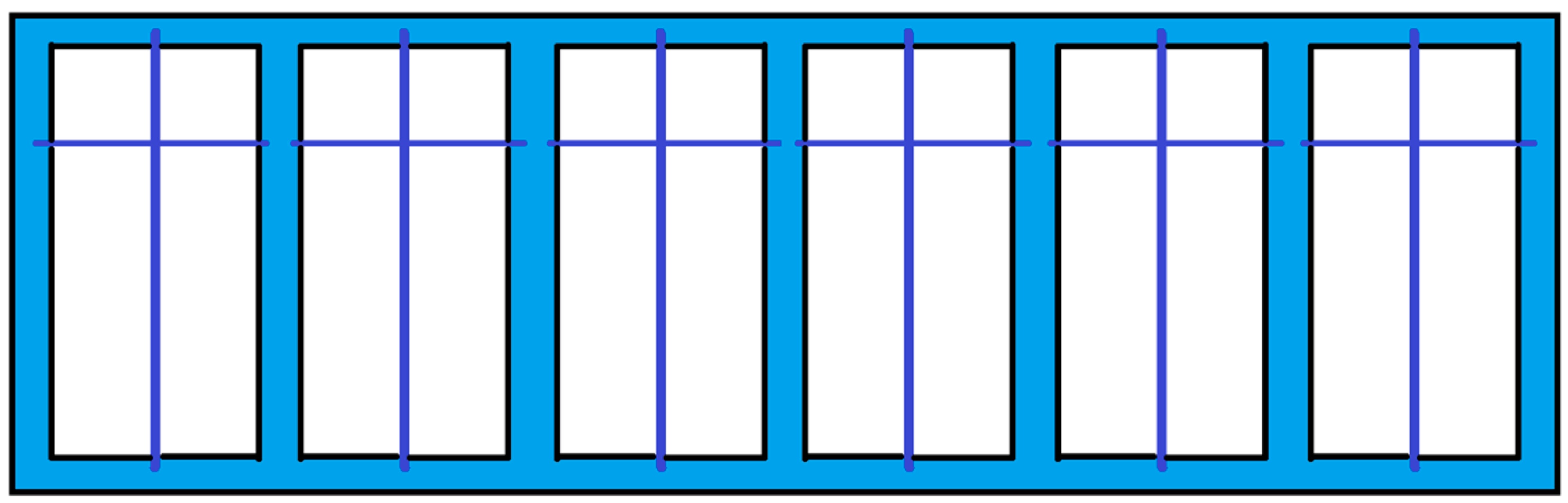
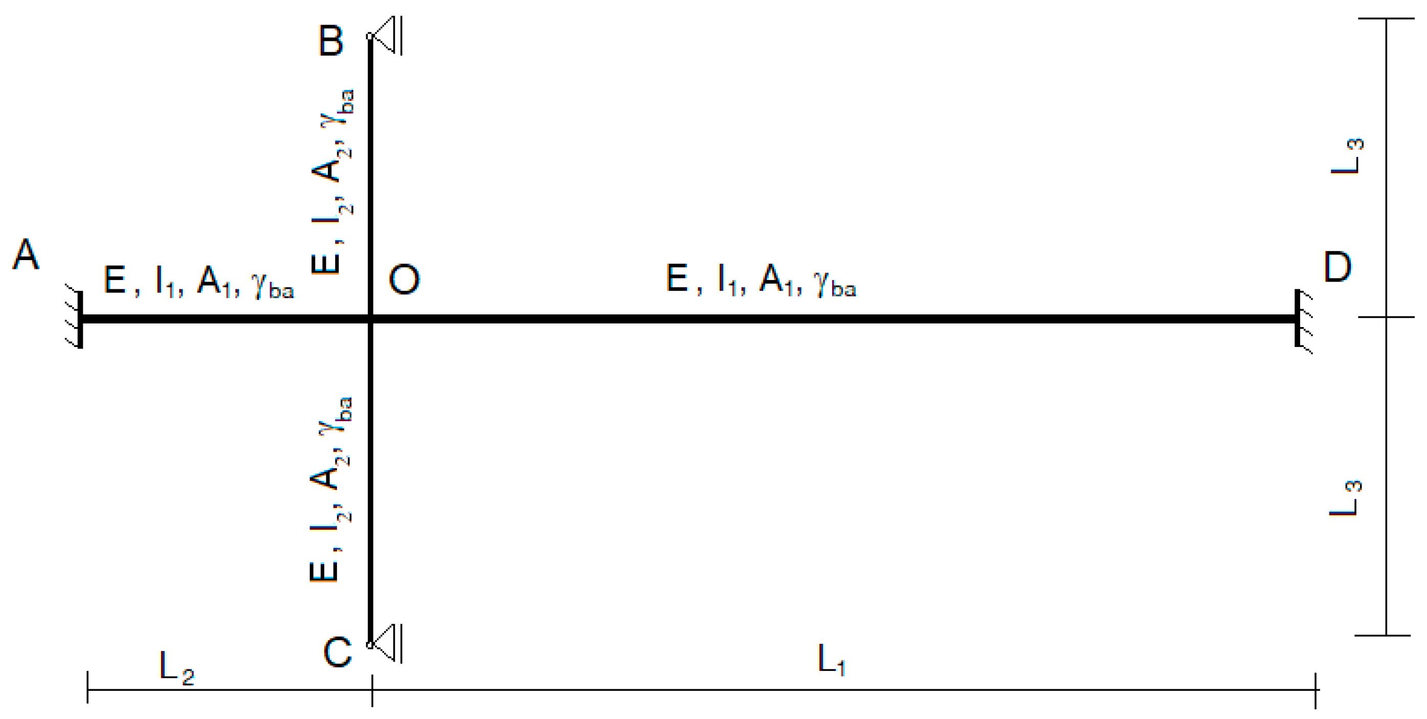
We have 2 coplanar reinforced concrete beams with different properties. AD beam is a main beam, considered double clamped at both ends, with the length L1 + L2. CB beam is a secondary beam, considered simply supported at both ends (nodes C and B), with length L3 + L3. The beams are made monolithically, so at point O of the intersection, a rigid knot is created. The secondary beam is arranged symmetrically to the main beam. The 2 beams have the Young’s moduli E1 and E2. The 2 beams have different sectional properties: for beam AD, we have the moment of inertia Iz1 and the area of section A1, and for beam CB, we have the moment of inertia Iz2 and the area of section A2, with the property that Iz1 > Iz2 and A1 > A2. The whole structure is presented in Figure 1.
Thus, the model of the mechanical system considered (Figure 2) consists of two identical trusses OB and OC rigidly fixed, perpendicular to a third bar AOD. The trusses can have transverse vibrations in a direction perpendicular to the ABDC plane and torsional vibrations. The trusses are clamped in the points B and C. In A and D, the AOD trusses are clamped, so the displacement, slope, and torsion angle at these points are zero. For point O, the transverse displacements of point O belonging to all four bars are equal. The torsion angle of the truss AO in O is equal to the torsion angle of the truss OD in O and with the slope of the bars OB and OC in O. The torsion angle of the trusses OB and OC in O is equal to the slope of the trusses AO and OD in point O. The sum of the shear forces and moments in O will be zero.
We will study a continuous concrete truss, homogeneous, with constant section. If there are no forces distributed or concentrated along the length of the truss, the vibrations of this are described by the well-known Equations [26]:
The notations used in Equation (1) are the following: v—is the truss deflection, A—s the cross section, is the mass density, E—Young’s modulus, and is the second area moment of inertia with respect to the z axis and x is the ordinate of the point having the deflection v.
Equation (2) must check Equation (1) at any time and, imposing this condition, we obtain:
Denote:
Then, Equation (1) becomes:
In Equation (5), represents the function, depending on the abscissa x, which gives us the deformed bar (eigenmode) corresponding to its eigenpulsation p. The solution is:
The constants are determined considering the boundary conditions for this problem.
In the following, we will use Equation (5) for the domains defined by the four trusses, obtaining, in this way, four differential equations of the fourth order, corresponding to the frames AO, OD, OB, OC (see Appendix A).
The study of torsional vibrations for a straight bar, unloaded over the length, leads to the second order differential equation:
where is the angle of torsion of the cross section being at the distance x from the end of the truss, is the polar moment of inertia, is the polar second moment of the area, and G is shear’s modulus.
The solution Equation (7) is sought in the form:
Equation (8) must verify Equation (7), from which we obtain:
where the notation was made:
The solution is:
Denoted by is the bending moment of a bar in section x, T the shear force that appears in the cross section and with the torque. For the studied system in the paper, the boundary conditions are:
- (a)
- For the AO truss, the end A is clamped, so: ; ;
- (b)
- For the OD truss, the end D is supported, so:
- (c)
- For the OB truss, the end B is supported so: ; ;
- (d)
- For the OC truss, the end C is clamped, so: ;
Imposing these conditions, for the considered four bars, 12 boundary conditions are obtained. The two moments and the shear force are expressed by the known relationships in the mechanics of the deformable solid [30,31,32,33]:
Using the Equation (12), the solutions presented in Appendixes, and the boundary conditions (a), (b), (c), and (d) result in 12 linear equations involving the unknown constants (Appendix A).
The continuity of the elastic system at point O leads to the following conditions: we have once that the displacements in C for all trusses: (three conditions), the slopes in O of the trusses AO and OD are equal to the torsion angle of the trusses OB and OC in: (three conditions), and the torsion angles of the bars AO and OD in O are equal to the slopes of the bar OB and OC in O: ) (three conditions). These mean nine conditions presented in the Appendix B, from which nine linear equations result.
Three more conditions are needed to obtain the constants in the written differential equations. They are obtained by considering the equilibrium of an infinitesimal element of the mass containing the point O.
The sum of the four shear forces in O must be zero, so:
A similar equilibrium relation is obtained for bending and torsional moments:
Writing these three conditions results in three linear equations (Appendix C). The unknowns are:
or:
In such way, a homogeneous linear system with 24 equations with 24 unknowns was obtained. In order to have other solutions besides the trivial solution zero, the determinant of the system must be zero. Putting this condition, the obtained eigenfrequencies of the system can be determined from the obtained equation.
The continuous models used in our studies are excellent for a classical analysis of such systems. The boundary conditions, written for these models, ultimately lead to a linear system of homogeneous equations. For this system to have a solution other than the trivial solution, zero, it is necessary that the system determinant be equal to zero. Imposing this condition leads to writing the characteristic equation that will provide, by solving, its eigenfrequencies of vibration. Once these values are known, then, we can determine your eigenmodes for these frequencies.
The matrix of the system can be written, in a concise form:
where the matrices are presented in Appendix C.
The condition:
offers the eigenvalues of the system of differential equations.
3. Properties of the Eigenvalues and Eigenmodes
Let us now consider one of the identical trusses OB and OC. The truss is clamped in O and supported in B (or C). Equations (1) and (7) are also valid for the OB bar (OC), with the boundary conditions:
For point O:
and for the point B(C):
The solution is:
for transversal vibrations and:
with the imposed boundary conditions for this case:
Using conditions expressed by Equations (28)–(31), it is now possible to determine the constants from the linear homogenous system:
where is the matrix determined by Equation (A76).
If the condition of the existence of non-zero solutions is set:
det (A11) = 0
It is now possible to obtain the eigenvalues of the truss OB (or OC).
The following theorems will be proved in the following:
Theorem 1.
The eigenvalues for the OB truss, clamped at one end and supported at the other, are also eigenvalues for the entire mechanical system.
Proof.
We must show that det (A) = 0 implies det (S) = 0. In reference [34], this property is proved in a more general case. It turns out that the property is valid in our case. □
It follows that the eigenvalues of a single truss in Appendix D, clamped at one end and supported at the other, are also eigenvalues of the composed system, clamped in A and D and with the ends B and C supported.
Using the matrix done by Equation (A76), and obtaining the eigenvalues for this matrix, the eigenmodes of deformations are obtained using Equation (A85). The following two theorems will be proved:
Theorem 2.
Proof.
For the eigenvalues obtained from Equation (33), the following system must be solved:
where:
Condition (36) implies that a vector can be found, such that:
Suppose that we determined this vector. Equation (35) becomes, after performing some simple calculations:
If we take into account Equation (37), the system of Equations (38)–(40) becomes:
From Equation (41), because, in general, , it follows immediately:
and introducing that in Equation (43), we obtain , a relation which verifies also Equation (42), if we take into account Equation (37). If is denoted, it results in Equation (34). □
Theorem 3.
For the other eigenvalues of the system, the eigenvectors are of the form:
Proof.
For the eigenvalues calculated, the system of Equation (35) must be solved, with or:
Subtracting (47) from (46), we get:
If , it results in and . □
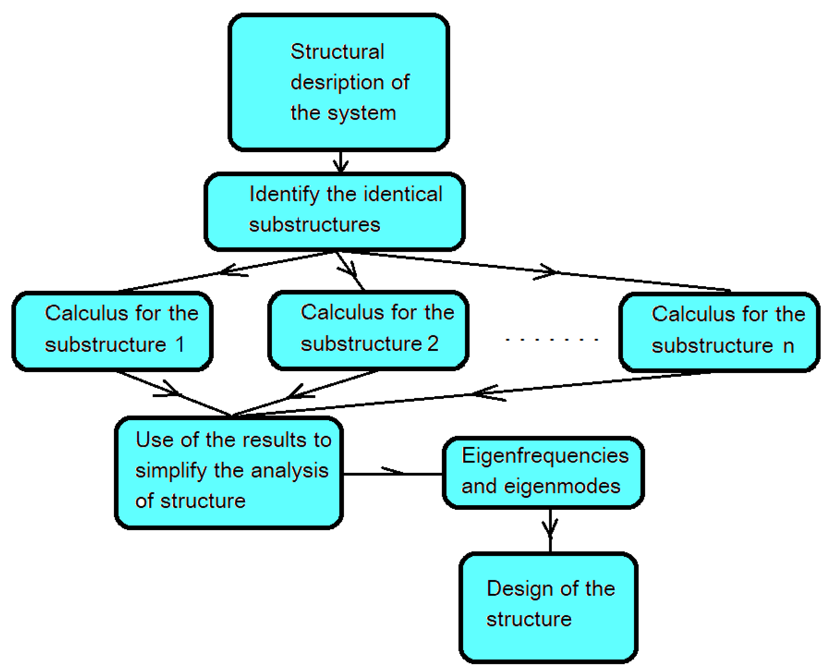
A block diagram representing the stage of the analysis is presented in Figure 4.
For the eigenfrequencies of the system that are the same with the eigenvalues of a single clamped truss at one end and supported at the other, the eigenmodes are skew symmetric, the two identical trusses vibrate in counterphase, and the third truss AOD rests. For the other eigenfrequencies, the identical trusses have identical eigenmodes.
4. Conclusions
Buildings and constructions, in general, show different forms of symmetry or are made up of repetitive elements. The existence of these symmetries leads to obtaining advantages related to the calculation, design, and manufacture of the structure. One of the advantages is related to the ease of describing the system by systematizing the information used; then, the properties demonstrated in the paper allow to decrease the time required to perform calculations and all this will allow savings and simplifications in the design process. Then, the existence of identical elements or identical parts can simplify the process of making the structure, by simplifying the labor and effort required to manufacture the structure. In conclusions, the design is simpler, and the realization costs are lower. There are also aesthetic reasons that justify the realization of structures with symmetries. From the point of view of calculation and behavior in static and dynamic cases, symmetries can bring significant advantages. In the strength of materials, symmetries are widely used in the static analysis of structures. However, they can be used for dynamic analysis, so that the vibrations of such structures allow simplification of the calculation and time savings in the design process. The paper has presented several vibration properties of a symmetrical structure made of concrete, used in civil engineering. Such structures are frequently encountered in the construction of buildings and in civil engineering and the knowledge of vibration properties can prove to be an advantage that allows to reduce the time and costs related to the design. We mention that symmetries appearing in all aspects of current life and in engineering applications are common. In consequence, the results obtained can be extended to other situations that may be encountered in practice. Future research could reveal other types of symmetries that will allow the systematization of the results and the proposal of a strategy to approach the design and execution of systems with identical parts or symmetries.
Author Contributions
Conceptualization, S.V., M.M., and O.D.; methodology, S.V.; validation, S.V., M.M., and O.D.; formal analysis, M.M.; investigation, S.V.; resources, O.D.; writing—original draft preparation, S.V.; writing—review and editing, S.V.; visualization, M.M. and O.D.; supervision, M.M.; project administration, O.D.; funding acquisition, O.D. All authors have read and agreed to the published version of the manuscript.
Funding
This research received no external funding.
Institutional Review Board Statement
Not applicable.
Informed Consent Statement
Not applicable.
Data Availability Statement
Not applicable.
Acknowledgments
We want to thank the reviewers who have read the manuscript carefully and have proposed pertinent corrections that have led to an improvement in our manuscript.
Conflicts of Interest
The authors declare no conflict of interest.
Appendix A
For the truss AO:
For the truss OD:
For the truss OB:
For the truss OC:
The following notations are made:
Using (A5), the four solutions for the four differential equations of order four (A1)–(A4) are:
For torsion, the notation was made:
Index 1 corresponds to trusses AO and OD and index 2 to trusses OB and OC. Applying Equation (8) for the four trusses studied, leads us to:
For torsional vibrations of the bar AO:
for torsional vibrations of the bar OD:
for torsional vibrations of the bar OB:
for torsional vibrations of the bar OC:
The solutions of the four equations (A11)–(A14) are:
The solutions contain 24 integration constants that will be determined considering the boundary conditions.
The two moments and the shear force are expressed by the known relationships in the mechanics of the deformable solid [26,27]:
However:
Truss AO:
Truss OD:
Truss OB:
Truss OC:
The following relations will be obtained:
which represent a system of 12 equations.
Appendix B
These nine conditions lead to nine relationships:
in which, together, (A35)–(A46) represent a system of 21 equations.
From (A47), we can obtain the equations:
From (A48), we can obtain the equations:
From (A49), we obtain:
Appendix C
Three more conditions are needed to obtain the constants in the written differential equations.
They are obtained by considering the equilibrium of an infinitesimal element of the mass containing the point O.
The sum of the four shear forces in O must be zero, so:
Replacing the expressions of the shear force determined for the four bars in O, we obtain:
With the notation:
we can write:
A similar equilibrium relation is obtained for bending and torsional moments.
Taking into account relations (27)–(43), we obtain:
Using (11)–(14) and (23)–(26), the results are:
This denoted:
This represents a system with 24 equations with 24 unknowns. From the system formed, we must determine the constants , , , , , , , , , , , , , , , , , , , . They will be denoted, in the following:
with:
A homogeneous linear system was obtained. In order to have other solutions besides the trivial solution zero, the determinant of the system must be zero. Putting this condition, the obtained eigenfrequencies of the system can be determined from the obtained equation.
Denote:
In the following, we denote:
where:
In this case, the matrix of the system can be written, in a concise form:
and the system becomes:
The condition:
offers the eigenvalues of the system of differential Equations (6)–(9) and (19)–(22).
det(A) = 0
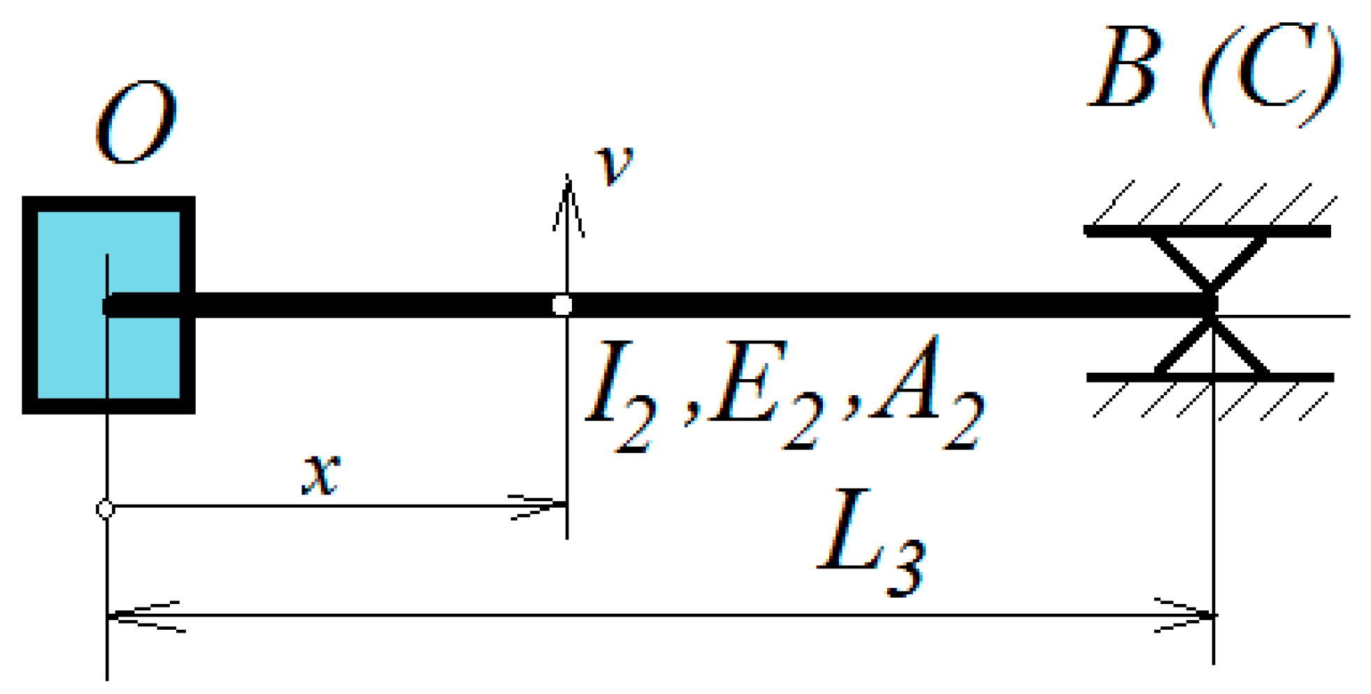
Appendix D
Let us now consider one of the identical trusses OB and OC. The truss is clamped in O and supported in B (or C). Equation (1) is also valid for the OB bar (OC), with the boundary conditions:
Figure A1.
Model of a single truss.

For point O:
and for the point B(C):
The solution:
offers the new equation:
If noted:
the solution is:
Torsional vibrations are described by Equation (15). By choosing as:
and introducing in Equation (15), we obtain:
The solution of the differential Equation (A93) will be:
References
- Meirovitch, L. Analytical Methods in Vibrations; McMillan: Hong Kong, China, 1967. [Google Scholar]
- Mihalcica, M.; Paun, M.; Vlase, S. The Use of Structural Symmetries of a U12 Engine in the Vibration Analysis of a Transmission. Symmetry 2019, 11, 1296. [Google Scholar] [CrossRef] [Green Version]
- Shi, C.Z.; Parker, R.G. Modal structure of centrifugal pendulum vibration absorber systems with multiple cyclically symmetric groups of absorbers. J. Sound Vib. 2013, 332, 4339–4353. [Google Scholar] [CrossRef]
- Paliwal, D.N.; Pandey, R.K. Free vibrations of circular cylindrical shell on Winkler and Pasternak foundations. Int. J. Press. Vessel. Pip. 1996, 69, 79–89. [Google Scholar] [CrossRef]
- Celep, Z. On the axially symmetric vibration of thick circular plates. Ing. Archiv. 1978, 47, 411–420. [Google Scholar] [CrossRef]
- Zingoni, A. A group-theoretic finite-difference formulation for plate eigenvalue problems. Comput. Struct. 2012, 112–113, 266–282. [Google Scholar] [CrossRef]
- Vlase, S.; Marin, M.; Oechsner, A. Considerations of the transverse vibration of a mechanical system with two identical bars. Proc. Inst. Mech. Eng. Part L J. Mater. Des. Appl. 2019, 233, 1318–1323. [Google Scholar] [CrossRef]
- Holm, D.D.; Stoica, C.; Ellis, D.C.P. Geometric Mechanics and Symmetry; Oxford University Press: Oxford, UK, 2009. [Google Scholar]
- Marsden, J.E.; Ratiu, T.S. Introduction to Mechanics and Symmetry: A Basic Exposition of Classical Mechanical Systems; Springer: Berlin, Germany, 2003; p. 586. [Google Scholar]
- Singer, S.F. Symmetry in Mechanics; Springer: Berlin, Germany, 2004. [Google Scholar]
- Zavadskas, E.K.; Bausys, R.; Antucheviciene, J. Civil Engineering and Symmetry. Symmetry 2019, 11, 501. [Google Scholar] [CrossRef] [Green Version]
- Ganghoffer, J.-F.; Mladenov, I. Similarity, Symmetry and Group Theoretical Methods in Mechanics; Lectures at the International Centre for Mechanical Sciences; Springer: Berlin, Germany, 2015. [Google Scholar]
- Lin, J.; Jin, S.; Zheng, C.; Li, Z.M.; Liu, Y.H. Compliant assembly variation analysis of aeronautical panels using unified substructures with consideration of identical parts. Comput. Aided Des. 2014, 57, 29–40. [Google Scholar] [CrossRef]
- Elkin, V.I. General-Solutions of Partial-Differential Equation Systems with Identical Principal Parts. Differ. Equ. 1985, 21, 952–959. [Google Scholar]
- Menshikh, O.F. Traveling Waves of a System of Quasilinear Equations with Identical Principal Parts. Dokl. Akad. Nauk USSR 1976, 227, 555–557. [Google Scholar]
- Zingoni, A. On the best choice of symmetry group for group-theoretic computational schemes in solid and structural mechanics. Comput. Struct. 2019, 223, 106101. [Google Scholar] [CrossRef]
- Zingoni, A. Group-theoretic insights on the vibration of symmetric structures in engineering. Philos. Trans. R. Soc. A Math. Phys. Eng. Sci. 2014, 372, 20120037. [Google Scholar] [CrossRef]
- Amaral, R.R.; Troina, G.S.; Fragassa, C.; Pavlovic, A.; Cunha, M.L.; Rocha, L.A.; dos Santos, E.D.; Isoldi, L.A. Constructal design method dealing with stiffened plates and symmetry boundaries. Theor. Appl. Mech. 2020, 10, 366–376. [Google Scholar] [CrossRef]
- Scutaru, M.L.; Vlase, S.; Marin, M.; Modrea, A. New analytical method based on dynamic response of planar mechanical elastic systems. Bound. Value Probl. 2020, 2020, 104. [Google Scholar] [CrossRef]
- Chen, Y.; Feng, J. Group-Theoretic Exploitations of Symmetry in Novel Prestressed Structures. Symmetry 2018, 10, 229. [Google Scholar] [CrossRef] [Green Version]
- Harth, P.; Beda, P.; Michelberger, P. Static analysis and reanalysis of quasi-symmetric structure with symmetry components of the symmetry groups C-3v and C-1v. Eng. Struct. 2017, 152, 397–412. [Google Scholar] [CrossRef]
- He, J.H.; Latifizadeh, H. A general numerical algorithm for nonlinear differential equations by the variational iteration method. Int. J. Numer. Methods Heat Fluid Flow 2020, 30, 4797–4810. [Google Scholar] [CrossRef]
- He, C.H.; Liu, C.; Gepreel, K.A. Low frequency property of a fractal vibration model for a concrete beam. Fractals 2021. [Google Scholar] [CrossRef]
- Ali, M.; Anjum, N.; Ain, Q.T.; He, J.H. Homotopy Perturbation Method for the Attachment Oscillator Arising in Nanotechnology. Fibers Polym. 2021, 22. [Google Scholar] [CrossRef]
- He, J.-H.; Hou, W.-F.; Qie, N.; Gepreel, K.A.; Shirazi, A.H.; Sedighi, H.M. Hamiltonian-based frequency-amplitude formulation for nonlinear oscillators. Facta Univ. Ser. Mech. Eng. 2021. [Google Scholar] [CrossRef]
- Den Hartog, J.P. Mechanical Vibrations; Dover Publications: Mineola, NY, USA, 1985. [Google Scholar]
- Thorby, D. Structural Dynamics and Vibrations in Practice: An Engineering Handbook; CRC Press: Boca Raton, FL, USA, 2012. [Google Scholar]
- Timoshenko, P.S.; Gere, J.M. Theory of Elastic Stability, 2nd ed.; McGraw-Hill: New York, NY, USA; London, UK, 2009. [Google Scholar]
- Tyn, M.U. Ordinary Differential Equations; Elsevier: Amsterdam, The Netherlands, 1977. [Google Scholar]
- Vlase, S.; Marin, M.; Scutaru, M.L.; Munteanu, R. Coupled transverse and torsional vibrations in a mechanical system with two identical beams. AIP Adv. 2017, 7, 065301. [Google Scholar] [CrossRef]
- Vlase, S.; Marin, M.; Öchsner, A.; Scutaru, M.L. Motion equation for a flexible one-dimensional element used in the dynamical analysis of a multibody system. Contin. Mech. Thermodyn. 2019, 31, 715–724. [Google Scholar] [CrossRef]
- Bhatti, M.M.; Marin, M.; Zeeshan, A.; Ellahi, R.; Abdelsalam, S.I. Swimming of Motile Gyrotactic Microorganisms and Nanoparticles in Blood Flow through Anisotropically Tapered Arteries. Front. Phys. 2020, 8, 95. [Google Scholar] [CrossRef] [Green Version]
- Nicolescu, A.E.; Bobe, A. Weak Solution of Longitudinal Waves in Carbon Nanotubes. Contin. Mech. Therm. 2021, 1–9. [Google Scholar] [CrossRef]
- Vlase, S.; Paun, M. Vibration analysis of a mechanical system consisting of two identical parts. Rom. J. Tech. Sci. Appl. Mech. 2015, 60, 216–230. [Google Scholar]
Figure 1.
Structure with repetitive cells.

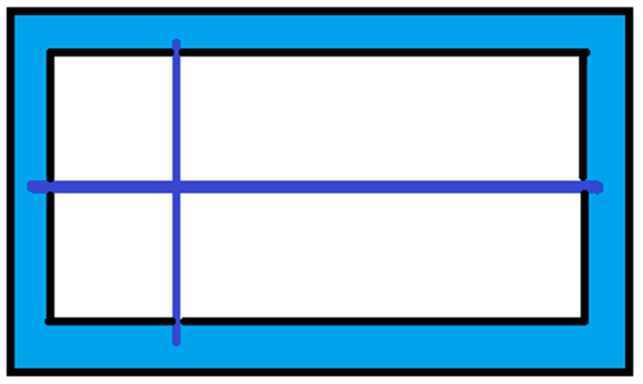
Figure 2.
One repetitive cell.

Figure 3.
Geometry of a repetitive cell.

Figure 4.
Block diagram of the operation.

Publisher’s Note: MDPI stays neutral with regard to jurisdictional claims in published maps and institutional affiliations. |
© 2021 by the authors. Licensee MDPI, Basel, Switzerland. This article is an open access article distributed under the terms and conditions of the Creative Commons Attribution (CC BY) license (https://creativecommons.org/licenses/by/4.0/).
Share and Cite
MDPI and ACS Style
Vlase, S.; Marin, M.; Deaconu, O. Vibration Properties of a Concrete Structure with Symmetries Used in Civil Engineering. Symmetry 2021, 13, 656. https://0-doi-org.brum.beds.ac.uk/10.3390/sym13040656
AMA Style
Vlase S, Marin M, Deaconu O. Vibration Properties of a Concrete Structure with Symmetries Used in Civil Engineering. Symmetry. 2021; 13(4):656. https://0-doi-org.brum.beds.ac.uk/10.3390/sym13040656
Chicago/Turabian StyleVlase, Sorin, Marin Marin, and Ovidiu Deaconu. 2021. "Vibration Properties of a Concrete Structure with Symmetries Used in Civil Engineering" Symmetry 13, no. 4: 656. https://0-doi-org.brum.beds.ac.uk/10.3390/sym13040656
Note that from the first issue of 2016, this journal uses article numbers instead of page numbers. See further details here.