Article

Numerical Analysis of the Flow Effect of the Menger-Type Artificial Reefs with Different Void Space Complexity Indices

Department of Fisheries College, Ocean University of China, Qingdao 266003, China
*
Author to whom correspondence should be addressed.
Xinxin Wang and Xianyi Liu contributed equally to this manuscript and should be considered co-first authors.
Submission received: 13 April 2021 / Revised: 7 May 2021 / Accepted: 11 May 2021 / Published: 9 June 2021
(This article belongs to the Special Issue Test and Measurement Technology in Ocean Engineering)

Abstract

:
Based on fractal theory, a regular fractal is used to construct symmetrical reef models (e.g., cube and triangle reef models) with different fractal levels (n = 1, 2, 3). Using the concept of fractal dimension, we can better understand the spatial effectiveness of artificial reefs. The void space complexity index is defined to quantify the complexity of the internal spatial distribution of artificial reefs models under different levels. The computational fluid dynamics (CFD) flow simulation approach was used to investigate the effects of void space complexity on the flow field performances of the symmetrical artificial reef models. The upwelling convection index ( H u p w e l l i n g / H A R , V u p w e l l i n g / V A R ), wake recirculating index ( L w a k e / L A R , V w a k e / V A R ) and non-dimensionalized velocity ratio range were used to evaluate the efficiency of the flow field effect inside or around artificial reefs. The surface area and spatial complexity index of artificial reefs increase with increasing fractal level. The numerical simulation data shows that the Menger-type artificial reef models with a higher spatial complexity index have better flow field performances in the upwelling and wake regions. Compared to the traditional artificial reef models, the upwelling convection index ( V u p w e l l i n g / V A R ) and recirculating index ( V w a k e / V A R ) of n = 3 fractal cube artificial reef increase by 37.5% and 46.8%, respectively. The efficiency indices of the upwelling region and wake region around the fractal triangle artificial reef model are 2–3 times those of the fractal cube artificial reef model when the fractal level is 3.

1. Introduction

In the 1960s the term “fractal” was first used by Benoit B. Mandelbrot [1] to describe complex geometry objects, which cannot be characterized by an integral dimension. Fractal geometry has been extensively applied in various fields (one-dimensional, 1D; two-dimensional, 2D; or three-dimensional, 3D), such as geophysics, biology, and fluid dynamics [2]. Application of the fractal in different ways leads to different results [3,4,5]. The concept of fractal sets proposed by Mandelbrot enables us to consider the degree of regularity of organizational structures associated with the behaviour of a physical system [6,7]. However, few studies have applied fractal theory in the design of artificial reefs (ARs). Fractals can be divided into regular and irregular fractals. The Sierpinski carpet is a typical representative of a regular fractal. The two important principles of fractal theory are the self-similarity principle and the iterative generation principle. Regular fractals are strict self-similar objects. Therefore, in this study, fractal theory was applied in the design of ARs with self-similar symmetrical structures, which could increase the structural complexity of ARs.
There are positive impacts on reef fishes abundance [8,9], species diversity and richness [9,10,11,12] by increasing the complexity of available habitat. Different habitat types and scales of ARs were deployed on the seabed, which can remove some environmental or ontogenic bottlenecks that may impact the nets’ yield gains in important commercial fishery productivity. The large surface area of ARs provides fishes with a place to forage, while the void spaces offer shelter from predation and wave surges. ARs with small void spaces and greater spatial structural complexity have greater fish abundance, species richness, and biomass than those with large void spaces [13,14]. Thus, the suitable design of the AR structure can effectively increase the productivity of some important commercial fish species [15]. Researchers such as Kim [16], have indicated that the variation configuration type and hole size offered by the porous ARs may also have effects on the fish assemblage. Therefore, the purpose of this study is to apply a regular fractal in the design of AR to improve the space validity and spatial complexity of reef bodies and provide numerous, relatively small interconnected cavities and an extended surface area. Shulman’s [17] experiments showed that the quantity and scale of sheltering places have significant impacts on the number, size, and species abundance of the reef fishes. Similarly, Eklund’s [18] observations indicated that the addition of concrete block rubble to generate void spaces inside reef structures can help increase the number of reef fishes, species, and biomass over hollow reefs. Sherman [13] carried out a two-year investigation to study the effects of block reef with highly complex void spaces and traditional reef ball with a simple large hollow space on the reef fishes abundance and species richness, respectively. His results showed that the block reef had higher biomass than the traditional reef ball. Overall, the application of fractal theory to improve the void space complexity of ARs is feasible.
One objective of this research was to quantify the complexity of the internal spaces distributed in an AR by calculating the void space complexity index (VSCI). As a quantitative feature and basic parameter, the fractal dimension (Df) is a crucial basic concept of fractal theory, which reflects the basic characteristics of fractals and the validity of the space occupied by complex shapes. The Df of the Menger sponge is between 2 and 3, i.e., approximately 2.727. It definitely is more than a 2D object, but it does not completely fill up 3D space. Therefore, how should the spatial validity and complexity of ARs be evaluated if a Menger sponge is applied in the design of ARs, such as a symmetrical cube or triangular ARs? At present, the geometric volume of an AR or reef set simply indicates the space scale occupied by the single AR or reef set, i.e., for a cube AR with side length a , the geometric volume is a 3 [19]. However, an AR unit is usually a structure with void space. In particular, some large ARs consist of a few interconnected chambers that can serve as physical sites for the settlement of fish larvae recruited from off-reef locations, and for foraging around the ARs. In this case, the geometric volume of an AR is not sufficient to reflect the void space complexity and validity. Here, the VSCI value of an AR mainly depends on two factors: the quantity and size of the void spaces in the reef body. The Menger sponge can be used to generate regular and symmetrical void space distribution inside an AR model, and the application of the Menger sponge in the design, making it easier to understand the formula for calculating the VSCI of an AR structure. In fact, the VSCI proposed in the present study can also be used to describe the structural complexity of irregular reefs or natural reefs; however, it is very hard to count the cavities and calculate their size in the irregular AR. Therefore, irregular or natural reefs are excluded from the scope of this paper.
Previous studies have stated that the existence of ARs can significantly affect the local flow distribution near the ARs by altering flow velocity, turbulence patterns, and sedimentary regimes, which can offer suitable fish habitat [20,21]. The change in flow velocity near the reefs, as an important factor for reef fishes aggregation effect blocks, is closely related to their size and configuration [22]. Computational fluid dynamics (CFD) simulation is a feasible tool for understanding the flow performance inside and around an AR model, which can be used to optimize the design of the structure and determine the effectiveness of AR deployment research [23,24,25]. Thus, to better understand the influence of spatial complexity of fractal ARs, numerical models were established to investigate the flow performance inside and outside fractal ARs with different VSCI values based on CFD methods. The numerical simulation results are expected to provide suggestions for the design of ARs with appropriate space complexity.
This paper is organized as follows. First, we apply fractal theory to design a Menger cube and triangle AR under different fractal orders, respectively. A quantified index, i.e., VSCI, is proposed to evaluate the structural complexity of ARs under different fractal levels. Second, the four cases were selected for detailed numerical analysis: a solid AR (n = 1), Menger ARs (n = 2,3), and traditional frame ARs. These simulation results can illustrate the relationship between the structural complexity and the flow field effect around ARs. Cost-benefit analyses were conducted following non-dimensionalized treatments, i.e., the convection efficiency index and recirculating efficiency index.

2. Menger-Type Artificial Reef Models and Numerical Simulation Methods

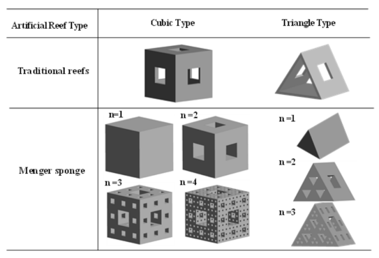
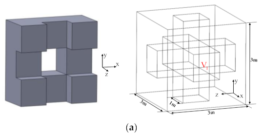
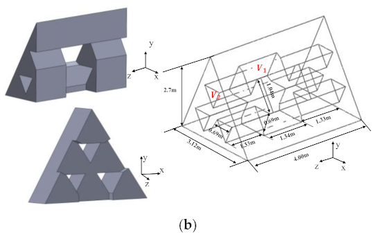
2.1. Menger-Type Artificial Reef Models

The Menger sponge is a type of regular fractal, which is an extension of the Sierpinski carpet in 3D space. ARs with complex spatial structures (i.e., Menger-type cube and Menger triangle ARs) were designed based on the Menger sponge model under different fractal levels (n = 1, 2, 3). Because the interior of the Menger sponge model is full of cavities of all sizes, the surface can reach an infinite size by continuously reducing the size of the holes. In 1919, mathematician Felix Hausdorff proposed the concept of continuous space, i.e., the dimension of space can change continuously; this can be a natural number, rational number, or positive irrational number, which is the Hausdorff dimension. Assuming that a self-similar fractal graph can be divided into N small graphs of the same size and shape, and the linear scale of each small graph is 1/r of the original graph, i.e., reduced by r times. The self-similar fractal dimension Df of this self-similar structure can be defined as the logarithmic ratio between the number N of the internal homotheties within a body and the reciprocal of the common ratio of the homothety r, see Equation (1) [1].
D f = ln N ( r ) / ln ( r ) .
For a 2D triangle with a fractal structure, the side length is 1/2 of the original triangle. The basic unit consists of N = 3 small triangles whose linear scale is narrowed to 1/2 of the original size, D f = ln 3 / ln 2 1.58 . For a 2D square with a fractal structure, the side length of each of the small square is 1/3 of the original square. The basic unit includes N = 8 small squares whose linear scale narrows to 1/3, D f = ln 8 / ln 3 1.893 . Therefore, for 2D fractal, the fractal dimension is between 0 and 2.
Next, we present the application of the Menger sponge in the design of a 3D symmetrical AR structure. Figure 1 shows the diagrams of the fractal cube and triangle ARs, respectively. Here, the fractal triangle reef combines square and triangle fractal methods, which significantly expands the surface area and improves the space complexity.
Starting with the level 1 cube, each subsequent iteration adds many small cubes within this level 1 cube. There are eight cubes at the front face, eight cubes at the back, and then four in between, for a total of 20 cubes (n = 20). Next, the length of each level 2 cube is 1/3 the length of the level 1 cube; hence, the magnification factor is 3. Using these values, the Df of the Menger cube AR is calculated as follows:
D f = ln 20 n / ln 3 n 2.727 .
The dimension of the Menger cube AR is between 2 and 3. It definitely is larger than a 2D object, but it does not completely fill up a 3D space either. Here, the Menger triangle AR is a special case, because it is a combination of a cube fractal and triangle fractal. According to the planar triangle fractal and 3D cube fractal, the total number of cubes and triangles is less than 20. Thus, Df of the Menger triangle AR should also be between 2 and 3.

2.2. Void Space Complexity Index

The VSCI is proposed to quantify the complexity of the internal space of an AR, which is determined by two factors: the number and size of the void space in the structure. The VSCI is defined as follows:
VSCI = i P i ( ln P i ) ,   i = 0 , 1 , 2 , 3 ,
where P i = V i / V , V i is the component volume of the void space in AR ( i = 0 , 1 , 2 , 3 ), V is the 3D volume of a fractal AR model including void spaces, as shown in Figure 2. With the increase of the fractal level, the interconnected chambers and surface area of AR also increase. That is to say, the higher the VSCI value is, the higher the void space complexity of the fractal AR model is. In Section 3.1, the detailed data of different component volumes in fractal AR models will be presented. In this paper, the prototype scale of the cube AR model is 3   m × 3   m × 3   m , and that of the triangle AR model is 4   m × 3.12   m × 2.7   m .

2.3. Numerical Simulation Methods

In terms of numerical calculations for flow field near ARs, CFD flow simulations are feasible tools to describe the flow vortex and flow fields inside and outside ARs, which can be useful to optimize the design of ARs. All CFD equations, in one form or another, are based on the fundamental governing equations of fluid dynamics—the equations of continuity, momentum, and energy [26]. In the present study, the Reynolds-averaged Navier–Stokes (RANS) equation was used to calculate the core performance function of the viscous fluid dynamics. The finite volume method (FVM) was applied to calculate the discretized RANs equation, which can improve the accuracy of the flow fields around submerged complex geometry and the computational efficiency of the computer programs [22].

2.3.1. Governing Equation

To simplify the numerical equations, it is assumed that the fluid in the flow field is an incompressible, steady, and viscous Newtonian fluid. The continuity equation and moment equation in the RANS equation can be expressed in the orthogonal coordinate system and are determined as follows,
The continuity equation:
ρ t + x j ( ρ u i ) = 0 ,
The momentum equation:
t ( u i ) + x j ( u i u j ) = p x i + x j μ u i x i ρ u i u j ¯ ,  
where u i is the mean velocity component (i = 1, 2, 3) for x, y, and z, respectively; p is the static pressure; u i and u j represent the fluctuating velocity, respectively; u i u j ¯ is the Reynolds stress; ρ is the fluid density, μ is the coefficient of the fluid dynamic viscosity. This study used the standard k ε turbulent flow model to replace u i u j ¯ , the related mathematical equations can be represented by the following equations:
t ( ρ k ) + x j ( ρ k u i ) = x j μ + μ t σ k k x j + G k ρ ε ,
t ( ρ ε ) + x j ( ρ ε u i ) = x j μ + μ t σ ε ε x j + C 1 ε k G k C 2 ρ ε 2 k ,
where G k represents the turbulent energy based on the average flow gradient; C μ , C 1 , and C 2 are constants; σ ε and σ k represent the turbulent Prandtl numbers for k and ε , respectively. These parameters can be expressed as follows [27]:
G k = μ t ( u i x j + u j x i ) u i x j , μ t = ρ C μ k 2 ε ,   C μ = 0.09 , C 1 = 1.44 , C 2 = 1.92 , σ k = 1.0 , σ ε = 1.3 .

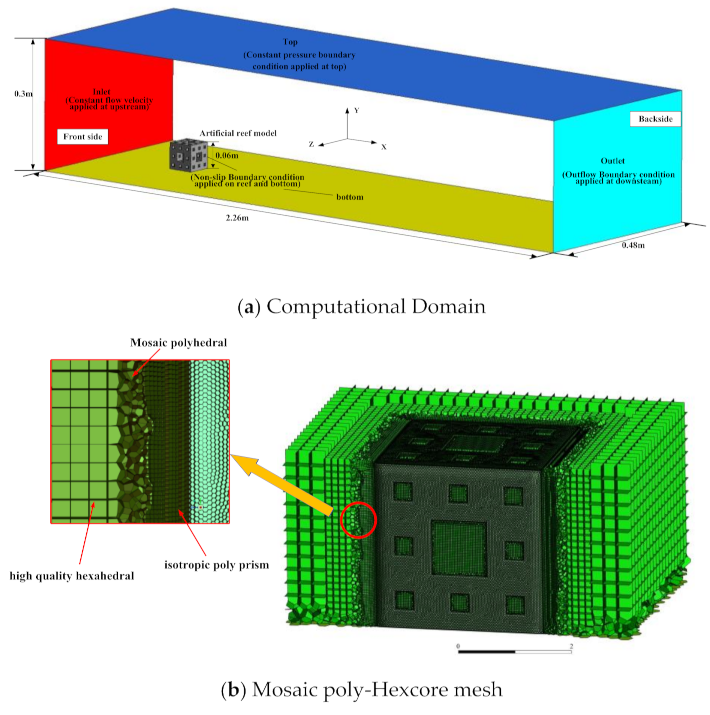
2.3.2. Computational Domain and Boundary Conditions

In the present study, the cube and triangle AR models are 1:50 scale models of the prototype models of the cube reef, and the triangle reef, respectively. Therefore, the model scale of the cube reef is 0.06   m × 0.06   m × 0.06   m (length × width × height), and the model scale of the triangle reef is 0.06 m × 0.08 m × 0.054 m (length × width × height). A computational domain of 2.26 m × 0.48 m × 0.3 m (length × width × height) was set in the Cartesian coordinate system, see Figure 3a. The AR model was placed in the middle of the computational domain. The width of the flow field around the AR model should be greater than 2.5 times the length of the AR model, to avoid the flow field being influenced by the sidewall effect [28]. The coordinate origin was set at the bottom centre of the reef 0.23 m upstream from the inlet and 2.03 m downstream from the outlet. The current speed around the Bohai Stain between Shandong Province and Liaoning Province of China is about 0.4 1.25 m/s. According to the Froude number, in the current study, the velocity in the simulation, 0.085 m/s, is also scaled by geometric scale, λ = 50. The boundary conditions were divided into inlet, outflow, and wall as follows:
(1)
The inlet was the fluid entrance of the computational domain, which is at the front side of the computational domain. The turbulent kinetic energy ( k ) and the turbulent dissipation ( ε ) were initialized at the inlet, respectively;
(2)
The outflow was applied behind the computational domain to model the flow outlet when the details of the flow velocity and pressure were unknown before solving the flow problem. This boundary condition is applicable when the flow is fully developed at the outlet;
(3)
The symmetry boundary conditions were applied in the sidewalls of the computation domain to model zero-shear slip walls in viscous flows. A fixed no-slip wall boundary condition was adopted at the bottom of the domain, in addition, the surface roughness coefficient of the ARs should also be considered during the simulation, which impacts its fluid dynamics and flow field [29,30,31]. Therefore, the AR surface faces were defined as a non-sliding wall with a roughness coefficient of 0.014.

2.3.3. Fluent Meshing Method

To obtain precise simulation results, it is necessary to construct the appropriate numerical model mesh. The mesh quality and mesh cells quantity are two main factors that directly affect the numerical simulation results. In general, the mesh should have low skewness (e.g., the maximum skewness less than 0.8) and high orthogonal quality (e.g., the minimum orthogonal quality greater than 0.2). However, a high mesh quality means more mesh cells and a longer computation time for the simulation. The Fluent meshing method used in the present study was developed to provide a native polyhedral mesh, which helps reduce the mesh count while preserving the mesh quality. This reduces the simulation time and resolves the boundary layer effect around ARs. It is integrated with Fluent to form a single-window workflow for CFD simulations (Fluent, 2012R1). In Fluent meshing, one can switch directly to the setup, solution, and post-processing modules.
In this study, the application of the Fluent Meshing method to the Menger-type AR grid process can generate efficient, high-quality meshes using the Mosaic Poly-Hexcore topology, which provides novel meshing strategies to solve the flow around increasingly complex ARs with greater accuracy and speed [32]. Furthermore, the technique is parallel and extensible on high-performance computing platforms and leads to faster grid mesh generation. It also speeds up the ANSYS Fluent solver by 10–50%, providing similar results and consuming less machine memory. Figure 3b shows the Poly-Hexcore with the Mosaic technology, in which the bulk region is filled by octree hexahedral elements, the boundary layer is filled by isotropic poly-prisms, and the transition region is filled by Mosaic polyhedron elements.
When meshing ARs, it is often useful to estimate the wall distance required to obtain the y + value. The grid near the AR wall must be accordingly sized to ensure accurate simulations. The first layer height is calculated according to the desired y + using flat-plate boundary theory. Due to the low Reynolds number (Re) and slow velocity in the boundary layer near the AR model, the standard k ε model could not be used to discretize the N-S equation directly. Therefore, a standard wall function was applied in the near-wall treatment, and a set of formulas were used to associate the boundary layer parameters with a Re and reference length to simulate the low Re flow in the boundary layer. According to the flow conditions and material characteristics, the following parameters are obtained:
Reynolds   number :   R e = ρ u l b o u n d a r y   l a y e r μ
Skin   friction :   C f = [ 2 log 10 ( R e ) 0.65 ] 2.3 for   R e < 10 9  
Wall   shear   stress :   τ w = C f 1 2 ρ u 2
Friction   velocity :   u τ = τ w ρ
Wall   distance :   Δ y = y + μ ρ u τ
where u is the inflow velocity and u τ is the wall friction velocity; τ w is the shear stress of the wall; l b o u n d a r y   l a y e r is the boundary layer length; C f is the skin friction coefficient related to Re. Δ y is first layer height near the reef wall. The y + of the turbulent flow is in the logarithm layer when y + ≥ 11.63. The properties of the logarithm layer are identical to those at the core of the turbulence. Consequently, the near-wall treatment was carried out when Δ y was arranged in the logarithmic layer and y + ≥ 11.63. In the present study, grid independence tests were carried out to obtain appropriate mesh size and mesh cells around the AR model [22,33]. The residuals convergence was set as 1 × 10 5 . Finally, the results of the tests show that for a cube AR model, the total number of mesh cells is about 1.0 × 10 6 1.9 × 10 6 , for a triangle AR model, the total number of mesh cells is about 1.2 × 10 6 1.9 × 10 6 . Table 1 lists the detailed data of grid size and cells amount for each simulation case. To enhance the numerical accuracy of the flow field, the minimum grid size was employed near the fractal reef block to mesh the fractal AR numerical model. Increasing the fractal orders, the total amount of the mesh cells increases.

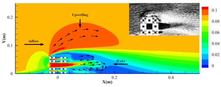
2.3.4. Flow Field Effects around an Artificial Reef

In this study, CFD numerical methods are effectively applied to describe the flow vortex and flow velocity distribution inside and outside the fractal AR models. With regard to the quantitative analysis of the influencing range of reef models, the flow field of the central cross-section plane (i.e., XOY central plane z = 0 or XOZ central plane y = 0.03 ) is more varied and complex [22]. Thus, the investigation of the AR flow field in the central plane facilitates comparisons of the flow performances by varying the fractal levels. Figure 4 presents the magnitude velocity contours in the central plane ( z = 0 ).
Upwelling region:
R u p w e l l i n g = ( x , y , z ) u y ( x , y , z ) > 0.1 u 0 ,   ( x , y , z ) C o m p u t a t i o n   D o m a i n ,
Wake region:
R wake = ( x , y , z ) u x ( x , y , z ) < 0 ,   ( x , y , z ) C o m p u t a t i o n   D o m a i n ,
Relative velocity region:
R relative = ( x , y , z ) 0 u ( x , y , z ) u 0 1 , ( x , y , z ) C o m p u t a t i o n   D o m a i n .
where u ( x , y , z ) is the fluid point velocity at ( x , y , z ) in the coordinate system, u 0 is the inflow velocity. u x is the component of velocity in the x-direction. u y is the component of velocity in the y-direction.
As shown in Figure 5, the upwelling height ( H u p w e l l i n g ) and upwelling volume ( V u p w e l l i n g ), and the wake length ( L w a k e ) and wake volume ( V w a k e ) were estimated to quantify the flow field efficiency to indicate the differences between the fractal AR models and traditional existing AR models. V w a k e can be estimated by adding all of the subvolumes with recirculating water flows, which are in the opposite direction to the flow direction. V u p w e l l i n g is estimated by adding all of the subvolumes with convection water flows, the local velocity component in the y-direction is greater than 0.1 u 0 . Thus, the upwelling and wake volumes include the corresponding finite volumes in and around the AR [34].

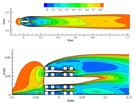
2.3.5. Flow Velocity Distribution Near an Artificial Reef

When an AR model was placed on the simulated seafloor, the field around the AR model showed a non-dimensionalized velocity value greater or less than 1.0, and the non-dimensionalized value away from the flow field near the AR model returned to nearly 1.0.
Tsung [22] carried out numerical analysis of the influence range of AR arrangements to emphasize that reef fishes aggregation was associated with the sheltering effects of slowing down the fluid movement behind the AR model. Similarly, in this study, the non-dimensionalized slow velocity distribution area with a value less than 0.8 could be obtained through numerical simulations. The effective range of the sheltering effect was used to compare the impact of the void space complexity of fractal reefs on the slowing velocity distribution.
To quantitatively determined the effective area of fractal AR models flow fields, the central plane (i.e., y c u b e = 0.03   m , y t r i a n g l e = 0.027   m ; z = 0 m) was used to present the nondimensionalized velocity distribution area, as shown in Figure 6. The related reference values can be calculated as follows:
α = u ( x , y , z ) u 0 , 0.1 α 0.8 ,  
A α = a r e a u ( x , y , z ) α u 0 ,  
k α = A α / A p ,  
where α is the non-dimensionalized velocity coefficient; A α is the non-dimensionalized velocity distribution area wherein the local velocity satisfied with u ( x , y , z ) α u 0 . k α is also a non-dimensionalized ratio between the non-dimensionalized velocity distribution area and projected area A p of the AR model.

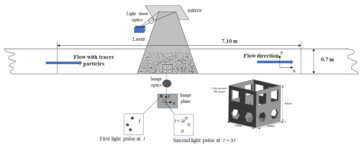
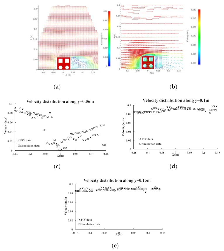
2.4. Particle Image Velocimetry (PIV) Experiments

To verify the accuracy of the numerical model, the particle image velocimetry (PIV) experiments of a symmetrical cube porous reef model were carried out in the flume tank at the Tokyo University of Marine Science and Technology. The tank measures 7 m × 0.3 m × 0.7 m (length × width × height), see Figure 7. The test reef model was placed in the middle of the test area. A large number of tracer particles (hollow glass beads with a diameter less than 10 μm and density close to that of water) tracked the flow movement. A green laser beam through a composite beam expander lens piece was used to illuminate the flow field, which was subsequently captured by a charge-coupled device (CCD) camera. The images captured by the CCD camera were analyzed with the PIVlab software to obtain the velocity distribution, vector, and streamlines, which were visualized by using Tecplot360 software.

3. Results

3.1. Void Space Complexity Index of Menger Type Artificial Reefs

Fractal cube and triangle AR models were constructed based on the fractal theory, which is expected to improve the space complexity and expand the surface area of ARs. For different fractal levels, the interconnected chambers inside the AR increased with the increase in the fractal order. Table 2 and Table 3 list the geometric parameters, such as concrete volume, surface area, interconnected chamber volume, and number for fractal cube and triangle AR models. We can obtain the VSCI value of each reef model by calculating Equation (3). From these data, we can conclude that the application of the fractal theory to construct ARs effectively improves the space complexity and expands the surface area. The VSCI value of fractal reef models is greater than those of traditional reef models.

3.2. Validation of Simulation Data

The numerical results for the four-opening cube reef model were validated by PIV measurements. Figure 8a–c represent the velocity distribution along y = 0.06 m, 0.1 m, and 0.15 m, respectively. The closer to the four-opening cube reef model, the fluctuation of the velocity curve is stronger. Figure 8 shows the comparison between the PIV experimental data and simulation data, which showed good agreement. Therefore, the numerical model (Standard kε model), the fluent meshing method (Mosaic poly-Hexcore mesh), and similar boundary conditions can be employed in the present study to simulate the flow around the Menger-type cube and triangle AR models.

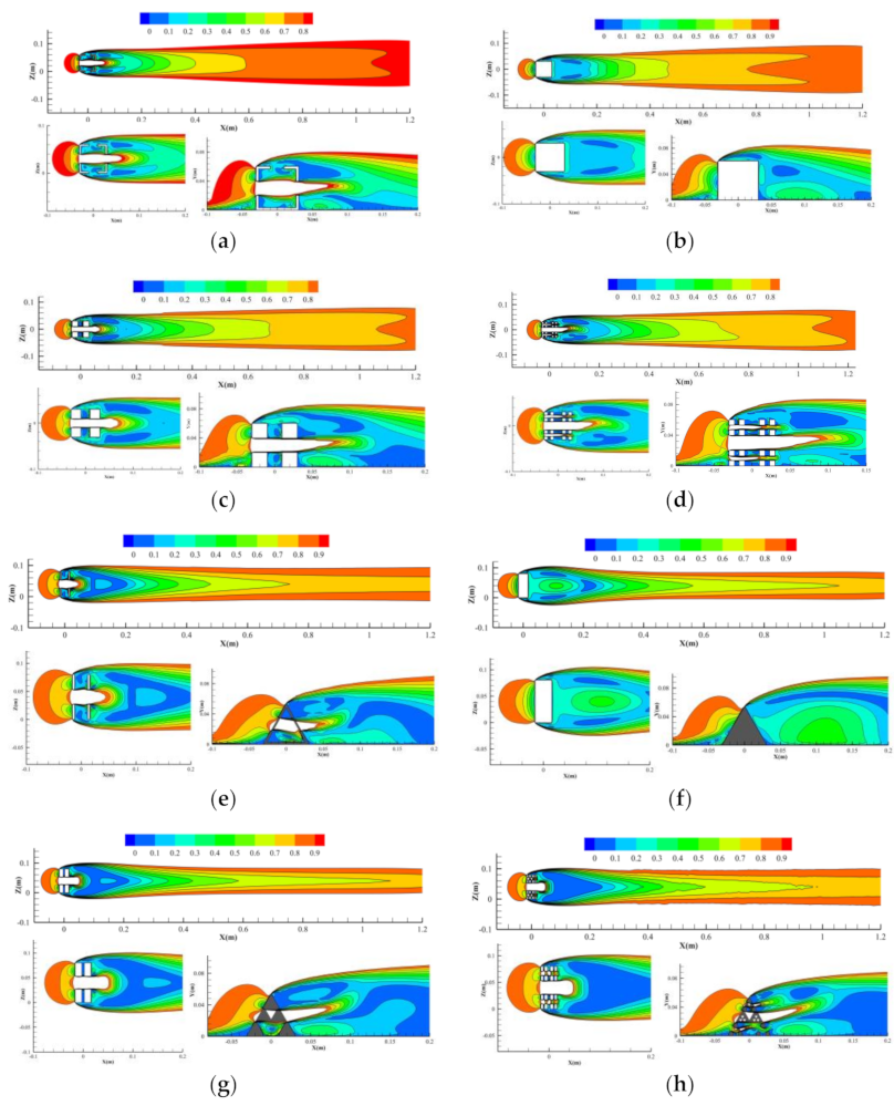
3.3. Flow Fields around Fractal Artificial Reef Models

The spatial complexity index values in Table 2 and Table 3 show that fractal AR models indeed have better structural complexity and connectivity performances as well as a greater surface area. However, the main function of ARs deployed on the sea bed is to change current speed and flow direction, which can generate various complex recirculating flows inside their bodies, to provide different flow conditions for fish aggregation [20].
In this section, the numerical simulations of the flow field inside and outside fractal AR models are carried out to describe the flow patterns around fractal AR models. The comparison between fractal and traditional reef models show the impact of the spatial complexity on the upwelling region, wake region and non-dimensionalized velocity influence range.

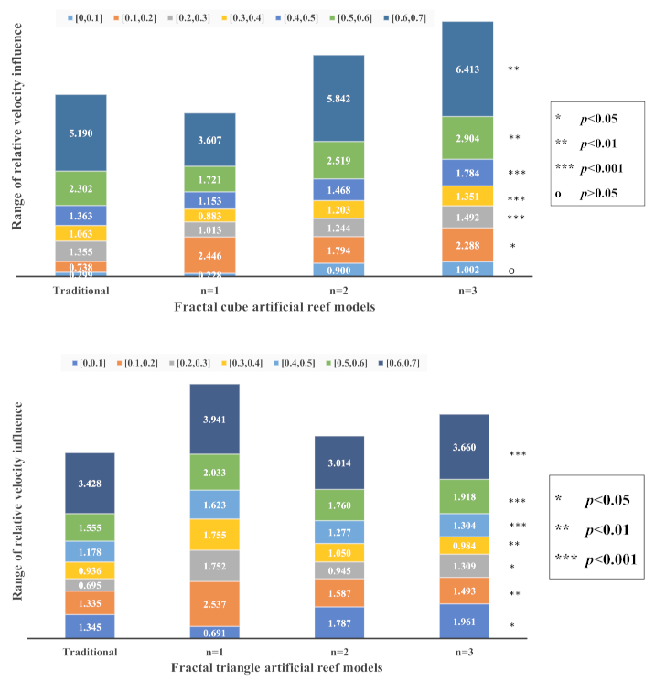
3.3.1. Non-Dimensionalized Slow Velocity Distribution of Flow Fields around the Fractal Cube Artificial Reef Models

Figure 9a–d present the nondimensionalized velocity distribution of the flow field around cube AR models under different fractal orders (n = 1, 2, 3). Table 4 lists the values of the non-dimensionalized area k α with a certain velocity contour line of relative velocity α behind the cube reef models. This value is the area of calculated equal-velocity line area divided by the projected area of the cube AR model (see Equation (16)), which is the square of the cube reef body length, 0.036 m2. For example, in Table 4, the value 26.806 under α 0.8 represents a non-dimensionalized area enclosed by all the domain points with a non-dimensionalized flow velocity α less than 0.8, for an n = 2 fractal cube AR model. As shown in Figure 9a–d, the velocity distribution contours show the significant differences between a simple traditional reef model and complex fractal reef models using CFD simulations. For a traditional frame and solid AR model (n = 1), which have no complicated inner space in their bodies, the area of low velocity behind them is less than that behind fractal reef models (n = 2, 3).
Figure 10a presents the non-dimensionalized low-velocity distribution column stacking diagram, 0 < α < 0.7 . If the plane covered by the equal velocity line was smaller than 0.7 times the inflow velocity defined as the sheltering effect of the AR, the influence range with a sheltering effect behind the AR model extended to approximately 10, 8, 12, and 13 times the reef length of the traditional and three fractal cube AR models, respectively. This indicates that within the range α < 0.7 , the area enclosed by velocity contour increases with higher fractal levels. Moreover, there was a significant difference among the four-cube reefs in the range α [ 0.2,0.5 ] , p < 0.001. With regard to the top and front views of the flow field near different fractal reef models, there are more complex recirculating flows inside the AR models with higher spatial complexity. The complex flow field can offer different velocity selection for fish habitats. According to the above analysis, the flow field effect around the solid AR model (n = 1) is the worst.

3.3.2. Non-Dimensionalized Slow Velocity Distribution of Flow Fields around the Fractal Triangle Artificial Reef Models

Figure 9e–h present the non-dimensionalized velocity distribution of the flow field around triangle AR models under different fractal orders (n = 1, 2, 3). Table 5 lists the value of the non-dimensionalized area coefficient k α with a certain velocity contour line of relative velocity α behind the triangle reef models. A comparison of the flow field simulation results among these four triangle reef models showed that, regardless of the non-dimensionalized velocity influence range or non-dimensionalized area, triangle AR models with high spatial complexity have better flow field effects and more complex recirculating flows inside their bodies, similar to fractal cube AR models. However, for the downstream side, the influence range of cube AR models per unit reef projected area is greater than that of triangle AR models. The area covered by the equal velocity line was 0.7 times less than the inflow velocity as the sheltering effect of the reef model. The influence range with a sheltering effect behind the triangle reef extended to approximately 12, 17, 18, 16 times the reef length of the traditional and fractal triangle AR models, respectively. Figure 10b presents the low-velocity distribution column stacking diagram ( 0 < α < 0.7 ). The sheltering effect differences ( 0.3 < α < 0.7 ) among fractal triangle AR models and traditional AR model were highly significant, p < 0.01.

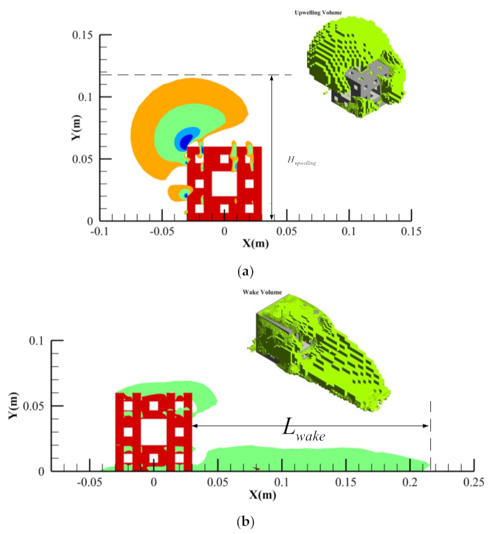
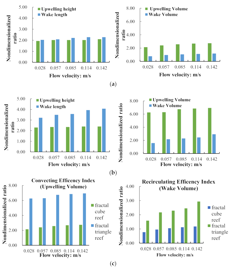
3.3.3. Upwelling Volume and Wake Volume

In Section 3.3.1 and Section 3.3.2, 2D analysis of the simulation data was employed to compare the influence range of cube and triangle AR models with different spatial complexities, respectively. The non-dimensionalized velocity distribution or non-dimensionalized area shows the flow field differences behind the reef models in the central plane. However, these 2D values are not sufficient to obtain the whole characteristics of upwelling and wake regions. The velocity distribution patterns and area of influence range were dependent on the selected analysis plane, e.g., the central plane. Therefore, the recirculating flows in or around an AR cannot be accounted for just by 1D or 2D measures. The wake volume, a 3D measure, proposed by Kim [35] was applied to quantify the scale of the wake region behind the AR model. Table 6 presents the 3D measures, upwelling volume, and wake volume. The value V u p w e l l i n g / V AR is the non-dimensionalized upwelling volume, i.e., the upwelling volume divided by the geometric volume of the AR model; for example, the geometric volumes of cube and triangle AR models are 2.16 × 10 4 m3 and 1.348 × 10 4 m3, respectively. For the upwelling and wake regions, the triangle AR model can generate greater upwelling and wake volume per unit geometric volume compared with the cube AR model. However, the non-dimensionalized velocity distribution in the central plane cannot indicate the differences between the two types of AR model. A comparison of the spatial complexity of cube and triangle AR models show that the index of the triangle AR model is greater than that of the cube AR model (see Table 2 and Table 3). Therefore, along with their higher spatial complexity, fractal triangle AR models have better upwelling and wake regions.
For the n = 1 case, the solid reef model had better upwelling and wake regions, but the recirculating and convection flows around the AR model were not better than in the other cases. Moreover, the solid AR was unable to provide sheltering places to protect fishes from predation. Therefore, we consider the cases (n > 1), fractal AR models with high spatial complexity can generate better upwelling and wake regions, and also provide more suitable habitats for reef fishes.

3.4. Effect of the Flow Velocity on the Flow Field around Fractal Artificial Reef Models

In this section, we study the impact of different inflow velocities on the flow field patterns around the fractal cube and triangle AR models. Reef models with fractal order of n = 3 were selected. The velocities were set to 0.028 m/s, 0.057 m/s, 0.085 m/s, 0.114 m/s, 0.142 m/s. Table 7 lists the velocities of the numerical model vs. the prototype model. To understand the impact of different velocities on the flow field inside and around the fractal AR models, the upwelling height, upwelling volume, wake length, and wake volume were calculated to quantify the flow effect inside and outside AR models, i.e., upwelling region and wake region.

3.4.1. Efficiency Indices of Upwelling and Wake Region of Fractal Cube Artificial Reef, n = 3

In this section, the impact of flow velocity on the upwelling and wake region of the fractal cube AR model (n = 3) was investigated. The upwelling height and wake length in the central planes, the upwelling volume and wake volume inside and around AR models were calculated according to the definition in Section 2.3.4. Table 8 shows no significant differences between the upwelling regions or wake regions inside or outside the cube AR model at various flow velocities.
To estimate the efficiency of the upwelling region or wake region as per the associated fabrication cost, four non-dimensionalized ratios ( H u p w e l l i n g / H A R , L w a k e / L A R , V u p w e l l i n g / V A R , and V w a k e / V A R ) were calculated under different flow velocities. These represent an efficiency index per unit length or per unit volume of fractal cube AR model [35]. Here, V A R is the geometric volume of the cube AR, 2.16 × 10 4   m 3 . The simulation results show no significant differences between the different flow velocities, which is consistent with our previous conclusion [24,25]. Figure 11a shows the efficiency indices of the upwelling region and wake region per unit length and per unit volume of the cube AR model. The efficiency indices of the upwelling height and wake length are 2.1 and 2.3, while the efficiency indices of the upwelling volume and wake volume are 2.7 and 1.1, respectively. The multidimensional data comparisons (1D, 2D, and 3D) reflect the flow patterns inside or outside AR models.

3.4.2. Efficiency Indices of Upwelling and Wake Region of Fractal Triangle AR Model, n = 3

Table 9 lists the upwelling height and wake length in the central planes, and the upwelling volume, and wake volume inside and around the n = 3 fractal triangle AR model at various flow velocities. Similar to the cube AR model, the change in flow velocity did not cause significant differences between the upwelling and wake regions. However, a comparison of the efficiency indices of the cube and triangle AR models showed that the structural shape was significantly different between these two regions. From Figure 9b, for the upwelling height and volume of the triangle reef model, the efficiency indices are 2.4 and 6.8, respectively, which are greater than those of the cube AR model, 2.1 and 2.7, respectively. In particular, for the upwelling and wake volumes, the efficiency indices are approximately 2–3 times those of the cube AR model (see Figure 11c). In Section 3.3, we analyzed the non-dimensionalized area ratios between the cube and triangle reef models. The simulation results indicate that the fractal triangle reef model with higher spatial complexity had better low-velocity distribution than the fractal cube reef model. These efficiency indices may be used as specific evaluation indices in the cost-benefit analysis of different AR structures. They also confirm the statement that “ARs play an important role in fisheries management.” [36]

4. Discussion

Structurally complex habitats are often shown to possess fractal characteristics [37,38,39]. The shortage of structurally complex elements in natural habitats exposes fish to predation [40]. Thus, in our study, the fractal theory was introduced as an optimized method to design an AR with a certain spatial complexity and extended surface area. When we consider fractal AR models with embedded cavities (n > 1), the fractal dimension Df of the artificial habitat was 2.727, which is more than a 2D but less than a 3D structure. For this novel structural model, our study quantified the space complexity of the Menger-type AR models and carried out numerical simulations to understand the flow field effect around fractal AR models. We applied the VSCI value to indicate the spatial effectivity differences among the fractal AR models under different fractal levels. CFD numerical simulation results show the convecting and recirculating efficiency indices of the flow field around the fractal cube and triangle AR models, respectively. Compared to the existing traditional AR models, the fractal AR models have greater VSCI values and better flow-field performance.
With regard to the fractal dimension Df of a 3D Menger AR model, we found that the same geometric structures have the same Df values for different fractal levels; in other words, all the 3D Menger cube AR models had the same Df value of 2.727. To demonstrate the relationship between the complexity of the reef structure and the fractal levels, we proposed a definition of the VSCI, which can evaluate the complexity of fractal ARs depending on the quantity and size of the interconnected cavities inside the AR bodies. The results show that the VSCI varied significantly among different fractal orders. When the fractal order is n 2 , both Menger cube and triangle AR models have greater VSCI values than the traditional AR models with a large hollow inside the reef. Under the same fractal order, the VSCI value of the Menger type triangle AR model is greater than that of the Menger type cube AR model. Overall, the above analysis of the VSCI values indicates that spatial complexity is an important factor in the construction of a well-designed reef structure.
As shown in Figure 1, fractals can generate different numbers and sizes of interconnected chambers inside an AR body. The detailed fractal information in Table 2 and Table 3 indicate that the fractal dimension determines the number of different-sized chambers inside the structure. With increasing fractal levels, the number of interconnected chambers increases, while the size of the subsequently generated chambers decreases. According to Sherman’s [13] and Eklund’s [18] observations, the reef blocks with spatial complexity can increase the reef fishes abundance, the fish species richness, and the biomass, compared to the traditional reef ball with a simple large hole space. Thus, we think that it is feasible to apply a high fractal level to improve and optimize the existing traditional AR structure. Because the different size chambers can provide suitable sheltering places for different marine reef fishes. Meanwhile, the extended surface area on the fractal AR models also can expand the functional role of the fractal reefs to attract more reef fishes to stay near the reefs for a long period through biofouling organisms. However, having more or larger chambers is not necessarily better. Hixon and Beets [41] found that an increase in the number of large shelters leads to an increase in the number of large predatory fish, which in turn leads to a decrease in the local abundance of small predatory fish. Therefore, this would suggest that it would be better to not intersperse large and small void spaces but have large voids in one area, and small voids in another. Thus the Menger sponge type of reef might not be suitable, since it has the different levels of voids evenly distributed. Thus, it is important to estimate the chamber size availability to optimize the cavity size before deploying well-designed ARs in the local environment.
Previous studies have indicated that deploying ARs in local marine environments can change the local flow velocity distribution inside and outside the reefs by varying the water flow, turbulence patterns, and sedimentary regimes, thereby creating suitable fish habitats [19,20,21,22,23,34]. Thus, this study carried out numerical simulations to further understand the effects of spatial complexity on the flow-field performance of the Menger-type reefs based on CFD. It is well known that the flow field around or behind the structure will change regardless of the shape of the structure deployed in the current. However, the flow patterns around and behind different structures were different. Even for the same structure or different sizes of the structure, the velocity variations behind the structure were different [42]. In Section 3.3, the non-dimensionalized velocity ratio was calculated to quantify the variation in the flow velocity when the current passed through the AR models. The contours of the non-dimensionalized velocity ratio visually represent the velocity distribution behind the fractal and traditional reef models. The flow field simulations clearly show the flow patterns inside and around these reefs’ blocks. The non-dimensionalized velocity values indicate the influence range of different velocities. Given the area covered by the equal velocity line, which is 0.7 times smaller than the inflow velocity, as the sheltering effect of the reef, Figure 9d,h show that the influence ranges of the flow field extended to approximately 13 and 16 times the reef lengths for n = 3 fractal cube and triangle ARs, respectively. However, the traditional cube and triangle AR models have an influence range of 10 and 12 times the reef lengths, respectively. Taken together, these simulation results show that fractal ARs can generate a complex flow field in which reef fishes can select a favourite velocity region as a comfortable living space. Meanwhile, the complex interconnected chambers can provide breeding grounds for reef fishes to protect them from predators. Our results support the importance of structural complexity in AR design to enhance fish recruitment, aggregation, and diversity [13,22].
Our numerical simulations of the flow field patterns inside or around the AR models can explain the significant differences between the fractal ARs and traditional ARs through nondimensionalized ratio values, e.g., convection efficiency indices ( H u p w e l l i n g / H A R , V u p w e l l i n g / V A R ) and recirculating efficiency indices ( L w a k e / L A R , V w a k e / V A R ). A comparison of the fluid effect or convection efficiency indices (e.g., upwelling height H u p w e l l i n g / H A R and upwelling volume V u p w e l l i n g / V A R ), recirculating efficiency (e.g., wake length L w a k e / L A R and wake volume V w a k e / V A R ) of fractal and traditional AR models, and the flow field efficiency indices showed that the fractal reefs with higher VSCI values have better performance in the upwelling and wake regions. From Figure 11c, it can be seen that the size of the upwelling region and the wake region around the fractal triangle AR model was greater than those of the fractal cube AR model. Therefore, a more detailed understanding of the relationship (e.g., the void space complexity, the influence range of the non-dimensionalized velocity, and the flow efficiency indices) will enable us to improve the design of complex reef structures to provide more suitable sheltering places to enhance fish recruitment, aggregation, and diversity.
In future work, we will carry out marine tests and structural optimization simulations to improve the fractal AR structures with more appropriate void spaces distributed inside reef bodies. These could be regular or irregular fractals, depending on the physical aspects of fractal AR design and their configuration and placement, which can facilitate and enhance the application of fractal ARs in fisheries. We anticipate establishing the relationship between the VSCI and the abundance or richness of marine fishery resources around ARs.

5. Conclusions

Our research successfully applied the fractal theory to create the Menger-type cube and triangle AR models. According to the non-dimensionalized VSCI values, the fractal AR models have greater VSCI values than the traditional AR model with a simple large hollow, and the surface area and VSCI of AR models increase with increasing fractal levels. At the same fractal level, the VSCI value of the fractal triangle AR model is greater than that of the fractal cube AR model. Moreover, the numerical simulation results show that the Menger-type AR models with a higher spatial complexity index have better flow field performances in the upwelling and wake regions. Compared to the traditional AR models, the upwelling convection index ( V u p w e l l i n g / V A R ) and recirculating index ( V w a k e / V A R ) of n = 3 fractal cube AR model increase by 37.5% and 46.8%, respectively. The efficiency indices of the upwelling region and wake region around the fractal triangle AR model are 2–3 times those of the fractal cube AR model when the fractal level is 3. Although our research does not support the actual use of fractal ARs to enhance and assemblage marine life on the fractal ARs, the VSCI values of the AR structure and numerical simulation results do support the importance of AR structure complexity in relation to void space in reef design.

Author Contributions

Void Space Complexity Index Conceptualization, X.L. and Y.T.; Methodology, X.W. and X.L.; validation, X.W. and X.L.; software simulation, X.L., X.W. and Y.L.; writing—original draft preparation, X.W. and X.L.; writing—review and editing, X.W. and F.Z. These authors contributed equally to this work. All authors have read and agreed to the published version of the manuscript.

Funding

This research was supported by National key R&D Program of China (Project No. 2019YFD0901302) and National Natural Science Foundation of China (Project No. 31802349; No. 32073025).

Institutional Review Board Statement

Not applicable.

Informed Consent Statement

Not applicable.

Data Availability Statement

Not applicable.

Acknowledgments

Not applicable.

Conflicts of Interest

The authors declare no conflict of interest.

References

  1. Mandelbrot, B.B. How long is the coast of Britain Statistical self-similarity and fraction dimension. Science 1967, 156, 636–638. [Google Scholar] [CrossRef] [Green Version]
  2. Rabault, J.; Sutherland, G.; Jensen, A.; Christensen, K.H.; Marchenko, A. Experiments on wave propagation in grease ice: Combined wave gauges and particle image velocimetry measurements. J. Fluid Mech. 2019, 864, 876–898. [Google Scholar] [CrossRef] [Green Version]
  3. Haralick, R.; Shanmugan, K.; Dinstein, I. Textural features for image classification. IEEE Trans. Syst. Man Cybern. 1973, 3, 610–621. [Google Scholar] [CrossRef] [Green Version]
  4. Pratt, W.; Faugeras, O.; Gagalowicz, A. Visual discrimination of stochastic texture fields. IEEE Trans. Syst. Man Cybern. 1978, 8, 796–804. [Google Scholar] [CrossRef]
  5. Panigrahy, C.; Seal, A.; Mahato, N.K. Image texture surface analysis using an improved differential box counting based fractal dimension. Powder Technol. 2020, 364, 276–299. [Google Scholar] [CrossRef]
  6. Mandelbrot, B. Fractals: Form. Chance and Dimension; Freeman: New York, NY, USA, 1977; 365p. [Google Scholar]
  7. Mandelbrot, B. The Fractal Geometry of Nature; Freeman: New York, NY, USA, 1983; 468p. [Google Scholar]
  8. Fujita, T.; Kitagawa, D.; Okuyama, Y.; Ishito, Y.; Inada, T. Comparison of fish assemblages among an artificial reef, a natural reef and a sandy-mud bottom site on the shelf off Iwate northern Japan. Environ. Biol. Fishes 1996, 46, 351–364. [Google Scholar] [CrossRef]
  9. Charbonnel, E.; Serre, C.; Ruitton, S.; Harmelin, J.-G.; Jensen, A. Effects of increased habitat complexity on fish assemblages associated with large artificial reef units (French Mediterranean coast). ICES J. Mar. Sci. 2002, 59, 208–213. [Google Scholar] [CrossRef] [Green Version]
  10. Fabi, G.; Fiorentini, L. Comparison between an artificial reef and a control site in the Adriatic Sea: Analysis of four years of monitoring. Bull. Mar. Sci. 1994, 55, 538–558. [Google Scholar]
  11. Gratwicke, B.; Speight, M.R. The relationship between fish species richness, abundance and habitat complexity in a range of shallow tropical marine habitats. J. Fish Biol. 2005, 66, 650–667. [Google Scholar] [CrossRef]
  12. Roberts, C.M.; Ormond, R.F.G. Habitat complexity and coral reef fish diversity and abundance on Red Sea fringing reefs. Mar. Ecol. Prog. Ser. 1987, 41, 1–8. [Google Scholar] [CrossRef]
  13. Sherman, R.L.; Gilliam, D.S.; Spieler, R.E. Artificial reef design: Void space, complexity, and attractants. ICES J. Mar. Sci. 2002, 59, S196–S200. [Google Scholar] [CrossRef]
  14. Anderson, T.W.; De Martini, E.E.; Roberts, D.A. The relationship between habitat structures body size and distribution of fishes at temperate artificial reef. Bull. Mar. Sci. 1989, 44, 681–697. [Google Scholar]
  15. Dean, L. Undersea oases made by man: Artificial reefs create new fishing grounds. Oceans 1983, 26, 27–29. [Google Scholar]
  16. Kim, H.B.; Lee, S.J. Hole diameter effect on flow characteristics of wake behind porous fences having the same porosity. Fluid Dyn. Res. 2001, 28, 449–464. [Google Scholar] [CrossRef]
  17. Shulman, M.J. Recruitment of coral reef fishes: Effects of distribution of predators and shelter. Ecology 1985, 66, 1056–1066. [Google Scholar] [CrossRef]
  18. Eklund, A. The Effects of Post-Settlement Predation and Resource Limitation on Reef Fish Assemblages. Doctoral Dissertation, University of Miami, Coral Gables, FL, USA, 1996. [Google Scholar]
  19. Yoon, H.S.; Kim, D.H.; Na, W.B. Estimation of effective usable and burial volumes of artificial reefs and the prediction of cost-effective management. Ocean Coast. Manag. 2016, 120, 135–147. [Google Scholar] [CrossRef]
  20. Pickering, H.; Whitmarsh, D. Artificial reefs and fisheries exploitation: A review of the ‘attraction versus production’ debate, the influence of design and its significance for policy. Fish. Res. 1997, 31, 39–59. [Google Scholar] [CrossRef]
  21. Lin, J.; Zhang, S.Y. Research advances on physical stability and ecological effects of artificial reef. Mar. Fish. 2006, 28, 257–262. [Google Scholar]
  22. Liu, T.L.; Su, D.T. Numerical analysis of the influence of reef arrangements on artificial reef flow fields. Ocean Eng. 2013, 74, 81–89. [Google Scholar] [CrossRef]
  23. Liu, Y.; Zhao, Y.P.; Dong, G.H.; Guan, C.T.; Cui, Y. A study of the flow field characteristics around star-shaped artificial reefs. J. Fluids Struct. 2013, 39, 27–40. [Google Scholar] [CrossRef]
  24. Tang, Y.L.; Long, X.Y.; Wang, X.X.; Zhao, F.F.; Huang, L.Y. Effect of reefs spacing on flow field around artificial reef based on the hydrogen bubble experiment. In Proceedings of the ASME2017 36th International Conference on Ocean, Offshore and Arctic Engineering, OMAE, Trondheim, Norway, 25–30 June 2017. [Google Scholar]
  25. Tang, Y.L.; Hu, Q.; Wang, X.X. Evaluation of flow field in the layouts of cross-shaped artificial reefs. In Proceedings of the ASME2019 38th International Conference on Ocean, Offshore and Arctic Engineering, OMAE, Glasgow, UK, 9–14 June 2019. [Google Scholar]
  26. Anderson, J.D. Computational Fluid Dynamics; McGraw-Hill Inc.: New York, NY, USA, 1995. [Google Scholar]
  27. Wang, F. Computational Fluid Dynamics Analysis; Tsinghua University Press: Beijing, China, 2004. (In Chinese) [Google Scholar]
  28. Lin, C.C. Numerical Study of Tank Wall Effect on Torpedo Flow. Master Thesis, CCIT, National Defense University, Taiwan, China, 2006. [Google Scholar]
  29. Colebrook, C.F. Turbulent flow in pipes with particular reference to the transition region between the smooth and rough pipe laws. J. Inst. Civ. Eng. 1939, 11, 133–156. [Google Scholar] [CrossRef]
  30. Shockling, M.A.; Allen, J.J.; Smits, A.J. Roughness effects in turbulent pipe flow. J. Fluid Mech. 2006, 564, 267–285. [Google Scholar] [CrossRef]
  31. Zhang, X.; Wang, G.; Zhang, M.; Liu, H.; Li, W. Numerical study of the aerodynamic performance of blunt trailing-edge airfoil considering the sensitive roughness height. Int. J. Hydrog. Energy 2017, 42, 18252–18262. [Google Scholar] [CrossRef]
  32. Zore, K.; Parkhi, G.; Sasanapuri, B.; Varghese, A. Ansys mosaic poly-hexcore mesh for high-lift aircraft configuration. In Proceedings of the 21st Annual CFD Symposium, Bangalore, India, 8–9 August 2019. (Conference paper). [Google Scholar]
  33. Wang, G.; Wan, R.; Wang, X.X.; Zhao, F.F.; Lan, X.Z.; Cheng, H. Study on the influence of cut-opening ratio, cut-opening shape, and cut-opening number on the flow field of a cubic artificial reef. Ocean Eng. 2018, 162, 341–352. [Google Scholar] [CrossRef]
  34. Kim, D.; Jung, S.; Kim, J.; Na, W.B. Efficiency and unit propagation indices to characterize wake volumes of marine forest artificial reefs established by flatly distributed placement models. Ocean Eng. 2019, 175, 138–148. [Google Scholar] [CrossRef]
  35. Kim, D.; Woo, J.; Yoon, H.S.; Na, W.B. Efficiency, tranquility and stability indices to evaluate performance in the artificial reef wake region. Ocean Eng. 2016, 122, 253–261. [Google Scholar] [CrossRef]
  36. Bortone, S.A.; Brandini, F.P.; Fabi, G.; Otake, S. Artificial Reefs in Fisheries Management; CRC Press & Taylor & Francis Group: Boca Raton, FL, USA; London, UK; New York, NY, USA, 2011. [Google Scholar]
  37. Mark, D.M. Fractal dimension of a coral reef at ecological scales: A discussion. Mar. Ecol. Prog. Ser. 1984, 14, 293–294. [Google Scholar] [CrossRef]
  38. Li, B.L. Fractal geometry applications in description and analysis of patch patterns and patch dynamics. Ecol. Model. 2000, 132, 33–50. [Google Scholar] [CrossRef]
  39. Purkis, S.J.; Kohler, K.E. The role of topography in promoting fractal patchiness in a carbonate shelf landscape. Coral Reefs. 2008, 27, 977–989. [Google Scholar] [CrossRef]
  40. Walters, C.J.; Juanes, F. Recruitment limitation as a consequence of natural selection for use of restricted feeding habitats and predation risk taking by juvenile fishes. Can. J. Fish. Aquat. Sci. 1993, 50, 2058–2070. [Google Scholar] [CrossRef]
  41. Hixon, M.A.; Beets, J.P. Shelter characteristics and Caribbean fish assemblages: Experiments with artificial reefs. Bull. Mar. Sci. 1989, 44, 666–680. [Google Scholar]
  42. Zhao, F.F.; Yin, G.; Muk, C.O. Numerical study on flow around partially buried tow-dimensional ribs at high Reynolds numbers. Ocean Eng. 2020, 198, 106988. [Google Scholar] [CrossRef]
Figure 1. Three-dimensional (3D) Menger-type cube and triangle artificial reef (AR) models.
Symmetry 13 01040 g001
Figure 2. The profile of level 2 fractal AR models. (a) presents the configuration of the level-2 fractal cube reef model; (b) presents the configuration of the level-2 fractal triangle reef model.
Symmetry 13 01040 g002aSymmetry 13 01040 g002b
Figure 3. (a) presents the computational domain and boundary conditions for AR flow numerical simulation; (b) presents the Mosaic poly-Hexcore mesh of the Menger cube AR.
Symmetry 13 01040 g003
Figure 4. Flow field velocity contour near AR in the central plane, z = 0.
Symmetry 13 01040 g004
Figure 5. Upwelling and wake regions: (a) presents upwelling height and upwelling volume; (b) presents wake length and wake volume.
Symmetry 13 01040 g005
Figure 6. The contour of the non-dimensionalized velocity distribution of fractal cube AR in the central plane, y = 0.03 m.
Symmetry 13 01040 g006
Figure 7. Particle image velocimetry (PIV) experiment flume tank and symmetrical four-opening cube porous reef model.
Symmetry 13 01040 g007
Figure 8. Comparison of the flow and velocity distribution line between the PIV model and numerical model. (a,b) are the velocity vector of the PIV model and numerical model, respectively; (c) is the velocity curve along y = 0.06 m; (d) is the velocity curve along y = 0.1 m; (e) is the velocity curve along y = 0.15 m.
Symmetry 13 01040 g008
Figure 9. Non-dimensionalized velocity contour with different fractal orders, n = 1,2,3. (ad) are the velocity contour of the fractal cube AR models; (eh) are the velocity contour of the fractal triangle AR models.
Symmetry 13 01040 g009
Figure 10. The non-dimensionalized ratio between the non-dimensionalized low-velocity area and projected area, k α .
Symmetry 13 01040 g010
Figure 11. Efficiency indices of n = 3 fractal cube and triangle AR models under different flow velocities. (a) presents the efficiency indices of n = 3 fractal cube AR model; (b) presents the efficiency indices of n = 3 fractal triangle AR model; (c) presents the comparison of efficiency indices between fractal cube and triangle AR models, n = 3.
Symmetry 13 01040 g011
Table 1. Grid allocations for fractal AR model flow simulations.
TypeFractal LevelMinimum Size (m3)Maximum Size (m3)Total Amount
Cuben = 14.33 × 10−117.08 × 10−61,009,446
n = 23.62 × 10−127.08 × 10−61,786,876
n = 31.30 × 10−137.08 × 10−61,876,488
Trianglen = 16.11 × 10−121.68 × 10−51,221,873
n = 22.49 × 10−121.68 × 10−51,600,308
n = 35.24 × 10−151.68 × 10−51,838,084
Table 2. Spatial complexity index of the Menger-type cube AR models.
Fractal
Dimension
DimensionConcrete
(m3)
Surface Area
(m3)
V 0 V 1
( 1,1,1 )
V 2
( 0.34,0.34,0.34 )
VSCI
n = 13 ×3 × 327.0045.000000
n = 23 ×3 × 320.0064.000700.572
n = 33 ×3 × 314.81112.14071400.896
Trad.
cube AR
3 ×3 × 36.5781.7320.43000.555
Table 3. Spatial complexity index of Menger-type triangle AR model.
Fraction OrderDimensionConcrete
(m3)
Surface Area
(m2)
V 0   V 1
3 Δ ( 0.69,0.69,1.04 ) h = 1.34   m
V 2
Δ ( 0.69,0.69,0.69 ) h = 1.33   m
V 3
Δ ( 0.2,0.2,0.26 ) h = 0.44   m
V 4
Δ ( 0.2,0.2,0.2 ) h = 0.44   m
V 5
Δ ( 0.2,0.2,0.2 ) h = 0.88   m
VSCI
n = 14 × 3.12 × 2.716.8533.360000000
n = 24 × 3.12 × 2.711.7854.180160000.801
n = 34 × 3.12 × 2.78.8491.620161554181.316
Trad. triangle
AR
4 × 3.12 × 2.74.7354.5712.12000000.594
Note: Δ ( 0.69,0.69,1.04 ) is the underside of a triangle prism with 0.69 m × 0.69 m × 1.04 m, the value in the column is the number of the triangle prism, see Figure 3.
Table 4. The non-dimensionalized area coefficient ( k α ) for different cube AR models.
Fractal Dimension α 0.1 α 0.2 α 0.3 α 0.4 α 0.5 α 0.6 α 0.7 α 0.8
n = 10.2282.6743.6884.5705.7237.44411.05126.806
n = 20.9002.6953.9395.1416.6099.12814.97033.734
n = 30.9943.2794.7686.1107.89210.78817.20434.948
Traditional type0.2991.0372.3923.4554.8187.12012.31031.539
Table 5. The non-dimensionalized area coefficient ( k α ) for different triangle AR models.
Fractal Dimension α 0.1 α 0.2 α 0.3 α 0.4 α 0.5 α 0.6 α 0.7 α 0.8
n = 10.6913.2284.9806.7368.35910.39214.33323.520
n = 21.7873.3744.3185.3686.6458.40511.41822.039
n = 31.9613.4544.7635.7477.0518.96912.62924.541
Traditional type1.3452.6803.3754.3115.4897.04410.47227.216
Table 6. Upwelling and wake volumes of cube and triangle AR models with different fractal orders.
Artificial TypeFractal Dimension V u p w e l l i n g ( m 3 ) V w a k e ( m 3 ) V u p w e l l i n g / V AR V w a k e / V AR
Cube n = 16.58 × 10−43.42 × 10−43.051.58
n = 25.45 × 10−42.01 × 10−42.520.93
n = 35.71 × 10−42.45 × 10−42.641.13
traditional 4.16 × 10−41.67 × 10−41.920.77
Triangle n = 11.27 × 10−37.22 × 10−49.465.36
n = 29.09 × 10−44.00 × 10−46.742.97
n = 39.08 × 10−43.09 × 10−46.742.30
traditional8.49 × 10−43.27 × 10−46.302.43
Table 7. Velocity condition for numerical model and prototype model.
Velocity (m/s)Case1Case2Case3Case4Case5
Numerical model0.0280.0570.0850.1140.142
Prototype0.198 0.403 0.601 0.806 1.040
Table 8. Upwelling height and volume, wake length and volume of n = 3 fractal cube AR model.
ScaleL = 0.06 m, H = 0.06 m, W = 0.06 m V u p w e l l i n g ( m 3 ) V w a k e ( m 3 ) H u p w e l l i n g ( m ) L w a k e ( m )
Velocity (m/s)0.0284.62 × 10−41.68 × 10−40.1160.122
0.0575.20 × 10−42.08 × 10−40.1210.125
0.0855.55 × 10−42.29 × 10−40.1210.133
0.1145.79 × 10−42.43 × 10−40.1210.137
0.1425.91 × 10−42.55 × 10−40.1260.137
Table 9. Upwelling height and volume, wake length and volume of n = 3 fractal triangle AR model.
ScaleL = 0.06 m, H = 0.054 m, W = 0.08 m V u p w e l l i n g
(m3)
V w a k e ( m 3 ) H u p w e l l i n g ( m ) L w a k e ( m )
Velocity (m/s)0.0288.43 × 10−42.14 × 10−40.124 0.193
0.0578.48 × 10−42.93 × 10−40.127 0.209
0.0859.08 × 10−43.09 × 10−40.127 0.214
0.1149.23 × 10−43.31 × 10−40.129 0.236
0.1429.35 × 10−43.95 × 10−40.129 0.244
Publisher’s Note: MDPI stays neutral with regard to jurisdictional claims in published maps and institutional affiliations.

