
Quantum Behavior of a Nonextensive Oscillatory Dissipative System in the Coherent State

Department of Nanoengineering, Kyonggi University, Yeongtong-gu, Suwon 16227, Gyeonggi-do, Korea
Symmetry 2021, 13(7), 1178; https://0-doi-org.brum.beds.ac.uk/10.3390/sym13071178
Submission received: 30 May 2021
/
Revised: 23 June 2021
/
Accepted: 26 June 2021
/
Published: 29 June 2021
(This article belongs to the Special Issue Symmetry Principles in Quantum Systems II)
Abstract
:We investigate the nonextensivity of a generalized dissipative oscillatory system in the Glauber coherent state. We introduce a parameter q as a measure of the nonextensivity of the system. Considering the characteristic of nonextensivity, the system is described by a deformed Caldirola–Kanai oscillator, which is represented in terms of q. We manage the system by describing the associated Hamiltonian in terms of the harmonic oscillator ladder operators. The time evolutions of the canonical variables, the Hamiltonian expectation value, the quantum energy, and the symmetry-breaking in the evolution of the system, are analyzed in detail regarding their dependence on q, damping factor, and the external driving force. The amplitude of the oscillator is slightly quenched as q becomes large, whereas the amplitude of the canonical momentum is enhanced in response to the growth in q. As q increases, the dissipation of the quantum energy becomes a little faster as a manifestation of the nonextensivity of the system. Our results are compared to the classical results, as well as to those in the previous research performed on the basis of the SU(1,1) coherent states. The coherent states, including the Glauber coherent states, can be convenient resources for carrying information, which is crucial in quantum information processing.
1. Introduction
The great success of Boltzmann–Gibbs (BG) statistics [1,2] is thanks to its general applicability in the description of the statistical properties of most physical systems. Boltzmann–Gibbs statistics provide a standard method for interpreting the thermostatistical behavior of ordinary dynamical systems based on ergodicity. This covers both the macroscopic and microscopic aspects. The principles of BG statistics also match strongly chaotic nonlinear dynamical systems. However, in spite of these potentialities of the BG statistics, it turned out that these statistics are not always applicable.
Some physical systems which exhibit nonextensivity in connection with multifractals and information theory do not follow BG statistics [3]. The meaning of “nonextensive” is “not extensive”, where “extensive” means naturally extendable/applicable to wide cases. The lesson associated with the study of nonextensivity is that the dynamical systems are not always ideal, but deviate from standard ones in some cases. Hence, the systems generalized along this line should inevitably be described by considering their nonextensive properties. The examples of physical phenomena associated with nonextensivity are long-range interactions [4,5], multifractals [6,7], microscopic memory [8,9], fluxes in cosmic rays [10], etc. The differences in the thermodynamical properties of the nonextensive dynamical systems and the usual extensive ones have been extensively explored to date.
Historically, nonextensive entropy as a modification of the usual entropy was introduced by Tsallis based on elegant multifractal concepts and structures as a generalization of thermostatistics [11]. After the Tsallis’s seminal report, much of the subsequent research in this context lead to quite interesting results for diverse properties related to nonextensivity [7,12,13,14,15,16,17,18]. At present, it is well-known in the physics community that Tsallis’s extension is suitable for describing peculiar characteristics of the nonextensivity of microcanonical and canonical ensembles.
For the case of general dissipative oscillatory systems, Özeren studied the nonextensive properties by introducing a deformed exponential function [18] in connection with the characterization of their coherent properties on the SU(1,1) basis. Özeren’s research is actually an extension of the Gerry’s investigation [19] for a dissipative system into the nonextensive regime. Afterwards, such a theoretical formalism for nonextensive dissipative systems was further elaborated by the present author [20,21], within the same basis of SU(1,1) algebra.
Motivated by the consequences of the above research, we will study the nonextensive properties of generalized dissipative oscillatory systems driven by an external time-varying force in the Glauber coherent state [22] in this paper. In order to study the nonextensivity of the system, we describe the time-dependent Hamiltonian for the damped driven oscillator in terms of ladder operators associated with the harmonic oscillator (HO). By introducing the nonextensivity parameter, the behavior of the system depending on that parameter will be analyzed in detail.
The organization of this paper is as follows. In Section 2, we describe the nonextensive damped harmonic oscillator through the Hamiltonian and the Langrangian formulations. Section 3 deals with the nonextensive properties related to the Glauber coherent state. Our consequences in the coherent state will be compared to those in the previous research, addressing the differences and similarities between them. We will show that our formulation of nonextensivity can be extended to quantum filed theory with a dissipative scalar field in Section 4. Finally, concluding remarks are given in Section 5. Through this research, we can learn the quantum dynamics associated with nonextensivity, which are applicable to the cases where the standard dynamics failed to reproduce the outcomes.
2. Mathematical Formulation
To clarify the nonextensivity characteristics of the generalized dissipative systems, we start from the Hamiltonian and Lagrangian formulation of the system. To unfold the quantum theory associated with nonextensive features of the systems, we introduce a deformed exponential function, which is known as q-exponential [18], such that
where . We express the dissipative system in terms of this exponential function. If , the system is superextensive, whereas it is subextensive when . For , Equation (1) reduces to an ordinary exponential function.
The nonextensive Caldirola–Kanai oscillator is represented by means of the Hamiltonian, which involves the q-exponential as
where is a damping factor and is an external driving force divided by mass. Note that given in Equation (2) is not a physical momentum, but a canonical momentum. The physical momentum, defined as , is also a useful quantity in the description of dissipative dynamical systems [23]. The relationship between the physical and the canonical momenta in this case is . The deviation of q from the unity is related to the degree of the nonextensivity.
From the study of dynamics associated with Equation (2), we can obtain a general representation of the mechanics, including the cases where a system is deviated from the standard behavior. For the case of , this Hamiltonian reduces to that of the usual dissipative-driven oscillatory system [24,25,26]. We elucidate the nonextensive properties of the quantum system described by this Hamiltonian.
Through the use of the annihilation operator
and its hermitian conjugate (creation operator), the Hamiltonian can be rewritten as
where
The eigenvalue equation of the annihilation operator is of the form
where and are the eigenvalue and the eigenstate, respectively. Here, the eigenstate is the Glauber coherent state which will be considered in this work. We can represent the expectation value of the Hamiltonian in the coherent state as
From the use of Equation (7), we have
For further development of the theory of the coherent state associated with the nonextensive system, it is useful to introduce the Langrangian. We consider the Langrangian which is defined in the form [27]
The Euler–Langrange equation of the system is given by
A minor evaluation after inserting Equation (10) into Equation (11) leads to
From the solution of this equation, it is possible to know how behaves in time. However, we do not know how to solve this equation analytically, even for the case where the explicit form of is given. As the best alternative plan, we will evaluate the eigenvalue numerically by using this equation in the subsequent section. Then, the nonextensivity of the system will be investigated based on the numerical consequence of .
3. Results and Discussion
As the coherent state is described in terms of , it is necessary to know the mathematical behavior of in order to see the nonextensivity properties in the coherent state. For convenience, we divide into real and imaginary parts as
where and are real. Then, the real and imaginary parts of Equation (12) are given, respectively, in the form
The solutions to these equations are different depending on . From now on, let us consider a particular case for further progress, which is that the external force is given by
where , , and are real. The parametric plots of and under the choice and the choice of as Equation (16) are given in Figure 1 and Figure 2, respectively. Figure 1A shows that the trajectory of the parametric evolution of and for a non-driven un-damped oscillator is symmetric from the origin. Such a symmetry is destroyed if there is a damping in the system (see Figure 1B,C). Nonextensivity of the system also acts as a source of symmetry-breaking. For the case of the superextensive () that is given in Figure 1B (red curve), the value of increases through the evolution compared to that in the absence of nonextensivity, whereas decreases. On the other hand, for the subextensive case () shown in Figure 1C (red curve), the plot exhibits the opposite behavior, which is that decreases whereas increases in comparison with the extensive case. If the damped nonextensive oscillatory system is driven by an external force, the parametric trajectory becomes somewhat more complicated, as can be seen from Figure 2.
In order to see the nonextensivity effects on coordinate and momentum, we represent them in terms of ladder operators as
Then, we easily obtain the expectation values of these operators in the coherent state such that
Figure 3 shows a delicate dependence of the time evolution of and on the degree of nonextensivity. The amplitude of decreases as q increases. On the other hand, the amplitude of increases as q becomes large. These consequences reflect the non-exponential behavior for the dissipation over time. Even if is not convergent in time, the expectation value of the physical momentum, , is convergent (see dash–dot curve in Figure 3B).
Although symmetry in parametric plots in Figure 1 and Figure 2 is broken by nonextensivity of the system, the symmetry between the positive and negative envelopes of the evolution of and is unbroken by nonextensivity (see Figure 3). However, Figure 4 shows that such a symmetry is broken by an external driving force.
If we define the fluctuation in an arbitrary operator as
it is not difficult to obtain the fluctuations in canonical variables: and . By multiplying these two outcomes, we obtain the uncertainty product in this model as , which corresponds to the minimum uncertainty product for canonical variables in quantum mechanics.
Now, let us see the quantum mechanical energy. It is known that the energy operator for a nonconservative system is somewhat different from the Hamiltonian [23]. The physical difference between the Hamiltonian and energy in this case is represented in Appendix A. For the case of the given system, the energy operator can be represented as [28,29]
The expectation value of this operator is given by . Then, using Equation (7), it is evaluated to be
This is the quantum energy in the Glauber coherent state in this model. Figure 5 and Figure 6 are the evolutions of the expectation value of the Hamiltonian and the quantum energy, where for Figure 5 and for Figure 6. These figures show the complicated behavoirs of Hamiltonian and quantum energy caused by the symmetry-breaking in the evolution of the system, which was mentioned previously. Although (quantum) energy dissipates in a somewhat irregular manner in this case due to the influence of the external force, the rate of dissipation is generally high whenever the oscillator moves rapidly in the vicinity of the equilibrium position ().
As q increases, the value of the Hamiltonian becomes larger, whereas the quantum energy becomes smaller in the same situation. The expectation values and deviate from those where the external force is absent as expected. For the case of the energy expectation value, such deviations are relatively large when is smaller than (this can be seen by comparing Figure 5B with Figure 6B).
The quantum energy is compared with those in the Perelomov’s SU(1,1) coherent states [30] in Figure 7. The formula of the quantum energies of the system in the SU(1,1) coherent states is represented in Appendix B for comparison purposes. It is well known that the allowed values of k in the SU(1,1) coherent states are and [30]. The quantum energy in the Glauber coherent state is larger than that in the SU(1,1) coherent state for the case that , while it is smaller than that in the SU(1,1) coherent state with .
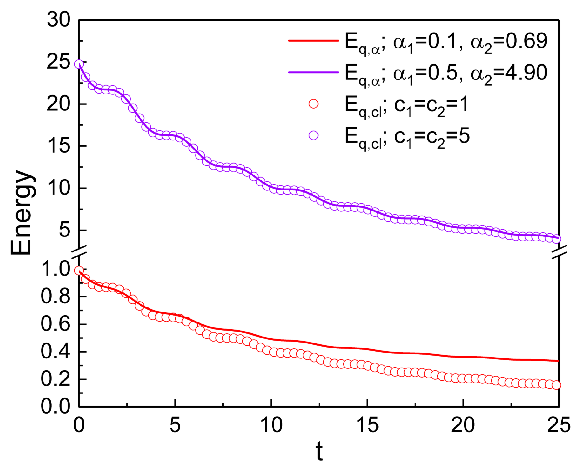
Now, we compare our results for the quantum energy in the Glauber coherent state with those of the classical energy. The classical energy of the system is represented in Appendix C. Figure 8 shows that the dissipation of quantum energy is slower than that of the classical energy provided that the initial energy is sufficiently small (see red curves in Figure 8). The reason the quantum energy does not significantly dissipate in the low-energy regime is the existence of the quantum zero-point energy. However, in the high-energy limit, the zero-point energy can be neglected because it is relatively small compared to the total energy. Hence, we can regard that the quantum energy is almost the same as that of the classical one in that limit (see violet curves in Figure 8), leading to quantum–classical correspondence.
4. Extension to Quantum-Field Description
In this section, we will show that our development can also be extended to a nonextensive description of quantum field theory for a scalar field that dissipates with time. The units, , will be used for simplicity throughout this section.
Let us consider a flat spacetime, of which the line element is given by
where is a time-varying scale factor. With this, it is possible to expand the scalar field with Fourier modes such that
where the two field components and are real. Then, the Hamiltonians for () can be represented as [31,32,33]
where . In the above equation, we have neglected the possible time dependence of . From this Hamiltonian, we have the equation for in the form
The solutions for this equation are different depending on the choice of the formula of . If we take
where is a real constant, the system becomes a nonextensive damped one, where the equation of motion is the same as the one we previously treated (see Equation (A7) in Appendix C):
Hence, all the developments performed up to the last section can be applied to this case, but under the condition .
5. Conclusions
The quantum characteristics of the nonextensive dissipative system, which is described by the q-exponential function, have been investigated. Nonextensive properties in the Glauber coherent state were analyzed through the representation of the system in terms of the HO annihilation and creation operators. Using the Euler–Langrange equation for ladder operators, we obtained the differential equation for (see, Equation (12)). Based on real and imaginary parts of that equation, the behavior of was analyzed and its dependence on q was addressed. The deviations of the behavior of several physical quantities in time can clearly be seen from the provided figures.
We have shown the nonextensivity effects for the expectation values of the canonical variables. As the nonextensivity parameter q increases, the amplitude of becomes slightly smaller whereas that of becomes larger at a given time. We have also shown how the symmetry in the evolution of the system is broken depending on the damping, nonextensivity, and external driving force.
The quantum energy of the damped nonextensive system dissipates as time goes by, as in the ordinary dissipative systems, but the rate of dissipation is a little different depending on the value of q. The dissipation of the quantum energy becomes slightly higher as q increases as a manifestation of the nonextensivity effects. Because dissipation is related to the damping factor physically, such a difference in dissipation rate implies that the damping factor is altered slightly depending on q.
We compared our results for the evolution of the quantum energy in the Glauber coherent state with those in other states, such as the SU(1,1) coherent states and the classical state. The quantum energies in both Glauber and the SU(1,1) coherent states dissipate in a similar way as expected. The dissipation pattern of the energy in the Glauber coherent state and in the classical state are also very much the same as each other in the high-energy limit. However, the dissipation of the quantum energy is slower than that of the classical energy in the case where the energy is very low, on account of the small intrinsic uncertainty in the quantum energy which gives the zero-point energy.
We have seen that the rate of dissipation is slightly different depending on q as a nonextensive behavior from our present work. On the other hand, the strength of the Tsallis formulation is that there is thermodynamic background of the nonextensive behavior of entropy [34,35,36]. Our work is related to the nonextensive dissipative phenomena of oscillatory systems characterized by q-exponential [18,20,21]. For the case of the Tsallis formulation, commutation relation is slightly altered depending on q. However, in our nonextensivity formalism for dissipative systems, commutation relation follows the standard rule, where q is only related to dissipation phenomena.
As a final remark, coherent states and entangled coherent states, including their generalization, can potentially be utilized in the quantum information processing technique [37,38,39]. Hence, characterizing and elucidating coherent states with their related phenomena, as well as the robust schemes for generating them, are important.
Funding
This work was supported by the National Research Foundation of Korea(NRF) grant funded by the Korea government(MSIT) (No.: NRF-2021R1F1A1062849).
Institutional Review Board Statement
Not applicable.
Informed Consent Statement
Not applicable.
Data Availability Statement
Not applicable.
Conflicts of Interest
The author declares no conflict of interest.
Appendix A. The Physical Difference between Hamiltonian and Energy
As is well known, the Hamiltonian and energy operator for a conservative system are the same as each other: they not only provide energy, but play the role of the generator of the equation of motion.
However, for a time-varying Hamiltonian system, their roles are not the same. The Hamiltonian, in that case, is only the generator of the equation of motion, whereas its expectation value is different from the energy. For a simple case where in the classical regime, we can easily confirm that the Hamiltonian (Equation (2)) produces the equation of motion
The derivation of this outcome is based on the basic Hamilton’s equations, which are and where H is the counterpart classical quantity of (Equation (2)) with .
On the other hand, the energy operator gives only the energy of the system, while we cannot derive an equation of motion from it. For a general mechanical system that is described by a time-dependent oscillator, the classical energy can be written as
Here, we have assumed that mass and the frequency depend on time. Using Hamilton’s equations, we can rewrite this in the form
If we replace classical variables x and p in the above equation with operators and , it becomes a quantum-mechanical energy operator. For the damped harmonic oscillator whose equation of motion is given by Equation (A1), we have the energy operator as
This can be extended to the nonextensive case in the text and the result coincides with Equation (22).
Appendix B. Energy Expectation Values in the SU(1,1) Coherent States
We briefly represent the quantum dynamics of the Perelomov’s SU(1,1) coherent states for the system, which appeared in Reference [21]. It is possible to evaluate these states on the basis of the HO ladder operators. We consider the case that for simplicity. In this case, the SU(1,1) coherent states of the system are given in terms of a time-dependent parameter which is the solution of the differential equation
Quantum mechanical energies in the SU(1,1) coherent states can also be given in terms of [21]:
where the allowed values of k are and . For more details along this line, see Reference [21].
Appendix C. Classical Mechanical Energy
For simplicity, we consider the case that . Then, the classical equation of motion of the system is of the form
If we denote the two independent solutions of this equation as and , they are given by [40,41]
where and are constants, and are the Bessel functions of the first and second kind with . The classical mechanical energy is given as
where and are the classical canonical coordinate and momentum that are represented in the form
Here, and are real constants.
References
- Županović, P.; Kuić, D. Relation between Boltzmann and Gibbs entropy and example with multinomial distribution. J. Phys. Commun. 2018, 2, 045002. [Google Scholar] [CrossRef]
- Tsallis, C. Some comments on Boltzmann-Gibbs statistical mechanics. Chaos Solitons Fractals 1995, 6, 539–559. [Google Scholar] [CrossRef]
- Tsallis, C. Thermostatistically approaching living systems: Boltzmann-Gibbs or nonextensive statistical mechanics? Phys. Life Rev. 2006, 3, 1–22. [Google Scholar] [CrossRef]
- Cannas, S.A.; Tamarit, F.A. Long-range interactions and nonextensivity in ferromagnetic spin models. Phys. Rev. B 1996, 54, R12661–R12664. [Google Scholar] [CrossRef] [Green Version]
- Nazareno, H.N.; De Brito, P.E. Long-range interactions and nonextensivity in one-dimensional systems. Phys. Rev. B 1999, 60, 4629–4634. [Google Scholar] [CrossRef]
- Mayoral, E.; Robledo, A. Multifractality and nonextensivity at the edge of chaos of unimodal maps. Phys. A Stat. Mech. Its Appl. 2004, 340, 219–226. [Google Scholar] [CrossRef] [Green Version]
- Lyra, M.L.; Tsallis, C. Nonextensivity and multifractality in low-dimensional dissipative systems. Phys. Rev. Lett. 1998, 80, 53–56. [Google Scholar] [CrossRef] [Green Version]
- Frigori, R.B. Nonextensive lattice gauge theories: Algorithms and methods. Comput. Phys. Commun. 2014, 185, 2232–2239. [Google Scholar] [CrossRef] [Green Version]
- Wedemann, R.S.; Donangelo, R.; De Carvalho, L.A.V. Nonextensivity in a memory network access mechanism. Braz. J. Phys. 2009, 39, 495–499. [Google Scholar] [CrossRef] [Green Version]
- Tsallis, C.; Anjos, J.C.; Borges, E.P. Fluxes of cosmic rays: A delicately balanced stationary state. Phys. Lett. A 2003, 310, 372–376. [Google Scholar] [CrossRef] [Green Version]
- Tsallis, C. Possible generalization of BG statistics. J. Stat. Phys. 1988, 52, 479–487. [Google Scholar] [CrossRef]
- Varela, L.M.; Carrete, J.; Muñoz-Solá, R.; Rodríguez, J.R.; Gallego, J. Nonextensive statistical mechanics of ionic solutions. Phys. Lett. A 2007, 370, 405–412. [Google Scholar] [CrossRef]
- Wei, L. On the exact variance of Tsallis entanglement entropy in a random pure state. Entropy 2019, 21, 539. [Google Scholar] [CrossRef] [Green Version]
- Obregón, O.; López, J.L.; Ortega-Cruz, M. On quantum superstatistics and the critical behavior of nonextensive ideal Bose gases. Entropy 2018, 20, 773. [Google Scholar] [CrossRef] [Green Version]
- Plastino, A.R.; Plastino, A. Stellar polytropes and Tsallis’ entropy. Phys. Lett. A 1993, 174, 384–386. [Google Scholar] [CrossRef]
- Boghosian, B.M. Thermodynamic description of the relaxation of two-dimensional turbulence using Tsallis statistics. Phys. Rev. E 1996, 53, 4754–4763. [Google Scholar] [CrossRef] [Green Version]
- Zamora, J.D.; Rocca, M.C.; Plastino, A.; Ferri, G.L. Dimensionally regularized Tsallis’ statistical mechanics and two-body Newton’s gravitation. Phys. A Stat. Mech. Its Appl. 2018, 497, 310–318. [Google Scholar] [CrossRef] [Green Version]
- Özeren, S.F. The effect of nonextensivity on the time evolution of the SU(1,1) coherent states driven by a damped harmonic oscillator. Phys. A Stat. Mech. Its Appl. 2004, 337, 81–88. [Google Scholar] [CrossRef]
- Gerry, C.C.; Ma, P.K.; Vrscay, E.R. Dynamics of SU(1,1) coherent states driven by a damped harmonic oscillator. Phys. Rev. A 1989, 39, 668–674. [Google Scholar] [CrossRef] [Green Version]
- Choi, J.R.; Yeon, K.H. Dynamics of SU(1,1) coherent states for the damped harmonic oscillator. Phys. Rev. A 2009, 79, 054103. [Google Scholar] [CrossRef]
- Choi, J.R. The effects of nonextensivity on quantum dissipation. Sci. Rep. 2014, 4, 3911. [Google Scholar] [CrossRef] [Green Version]
- Glauber, R.J. Coherent and incoherent states of the radiation field. Phys. Rev. 1963, 131, 2766–2788. [Google Scholar] [CrossRef]
- Um, C.-I.; Yeon, K.-H.; George, T.F. The quantum damped harmonic oscillator. Phys. Rep. 2002, 362, 63–192. [Google Scholar] [CrossRef]
- Caldirola, P. Porze non conservative nella meccanica quantistica. Nuovo Cimento 1941, 18, 393–400. [Google Scholar] [CrossRef]
- Kanai, E. On the quantization of dissipative systems. Prog. Theor. Phys. 1948, 3, 440–442. [Google Scholar] [CrossRef]
- Choi, J.-R. Unitary transformation approach for the phase of the damped driven harmonic oscillator. Mod. Phys. Lett. B 2003, 17, 1365–1376. [Google Scholar] [CrossRef]
- Zhang, W.-M.; Feng, D.H.; Gilmore, R. Coherent states: Theory and some applications. Rev. Mod. Phys. 1990, 62, 867–927. [Google Scholar] [CrossRef]
- Yeon, K.H.; Um, C.I.; George, T.F. Coherent states for the damped harmonic oscillator. Phys. Rev. A 1987, 36, 5287–5291. [Google Scholar] [CrossRef]
- Dybiec, B.; Gudowska-Nowak, E.; Sokolov, I.M. Underdamped stochastic harmonic oscillator driven by Lévy noise. Phys. Rev. E 2017, 96, 042118. [Google Scholar] [CrossRef] [Green Version]
- Perelomov, A.M. Coherent states for arbitrary Lie group. Commun. Math. Phys. 1972, 26, 222–236. [Google Scholar] [CrossRef] [Green Version]
- Carvalho, A.M.D.M.; Furtado, C.; Pedrosa, I.A. Scalar fields and exact invariants in a Friedmann-Robertson-Walker spacetime. Phys. Rev. D 2004, 70, 123523. [Google Scholar] [CrossRef]
- Pedrosa, I.A.; Furtado, C.; Rosas, A. Exact linear invariants and quantum effects in the early universe. Phys. Lett. B 2007, 651, 384–387. [Google Scholar] [CrossRef] [Green Version]
- Choi, J.R. An approach to dark energy problem through linear invariants. Chin. Phys. C 2011, 35, 233–242. [Google Scholar] [CrossRef]
- Macfarlane, A.J. On q-analogues of the quantum harmonic oscillator and the quantum group SU(2). J. Phys. A Math. Gen. 1989, 22, 4581–4588. [Google Scholar] [CrossRef]
- Biedenharn, L.C. The quantum group SU(2) and a q-analogue of the boson operators. J. Phys. A Math. Gen. 1989, 22, L873–L878. [Google Scholar] [CrossRef]
- Márkusa, F.; Gambár, K. Q-boson system below the critical temperature. Phys. A 2001, 293, 533–539. [Google Scholar] [CrossRef]
- Jeong, H.; Kim, M.S. Efficient quantum computation using coherent states. Phys. Rev. A 2002, 65, 042305. [Google Scholar] [CrossRef] [Green Version]
- Bukhari, S.H.; Aslam, S.; Mustafa, F.; Jamil, A.; Khan, S.N.; Ahmad, M.A. Entangled coherent states for quantum information processing. Optik 2014, 125, 3788–3790. [Google Scholar] [CrossRef]
- Israel, Y.; Cohen, L.; Song, X.-B.; Joo, J.; Eisenberg, H.S.; Silberberg, Y. Entangled coherent states created by mixing squeezed vacuum and coherent light. Optica 2019, 6, 753–757. [Google Scholar] [CrossRef]
- Choi, J.R.; Lakehal, S.; Maamache, M.; Menouar, S. Quantum analysis of a modified caldirola-kanai oscillator model for electromagnetic fields in time-varying plasma. Prog. Electromagn. Res. Lett. 2014, 44, 71–79. [Google Scholar] [CrossRef] [Green Version]
- Choi, J.R. Quantum dynamics for the generalized Caldirola-Kanai oscillator in coherent states. IIOAB J. 2014, 5, 1–5. [Google Scholar]
Figure 1.
The parametric plot of Equations (14) and (15) with the absence of the driving force (), where (A) and (B,C). The dashed black curves in (A–C) are for the extensive cases (). On the other hand, the red curves in (B,C) are nonextensive cases: for A and for (B). The initial condition is chosen as (, ) = (1, 0) for all curves. The plot time for (A) is (, ) (0, 2), which corresponds to the evolution of a cycle (this time interval is enough in this case due to the regularity of the evolution), whereas the plot time for (B,C) is (, )(0, 23). We used , , and .

Figure 2.
Panels (A,B) are the same as Figure 1B,C respectively, but with a sinusoidal driving force (Equation (16)) where the chosen parameters are , , and .

Figure 3.
Time evolution of (A) and (B) for several different values of q where . An extra curve (dash-dot curve) is with . We used , , , and .
Figure 3.
Time evolution of (A) and (B) for several different values of q where . An extra curve (dash-dot curve) is with . We used , , , and .

Figure 4.
This figure is the same as Figure 3, but with a sinusoidal driving force (Equation (16)) where , , and . Time evolution of (A) and (B) for several different values of q where .

Figure 5.
Time behavior of the Hamiltonian (A) and the energy expectation value (B) in the coherent state for several different values of q. We used , , , , , , and . We note that this graphic corresponds to the case where .
Figure 5.
Time behavior of the Hamiltonian (A) and the energy expectation value (B) in the coherent state for several different values of q. We used , , , , , , and . We note that this graphic corresponds to the case where .

Figure 6.
This figure is the same as Figure 5, but for ; this choice of corresponds to the case of . Time behavior of the Hamiltonian (A) and the energy expectation value (B) in the coherent state for several different values of q.
Figure 6.
This figure is the same as Figure 5, but for ; this choice of corresponds to the case of . Time behavior of the Hamiltonian (A) and the energy expectation value (B) in the coherent state for several different values of q.

Figure 7.
Comparison for the time evolution of the quantum energy in the Glauber coherent state (solid curves) with those in the SU(1,1) coherent states (symbols) for (red) and (violet). We used , , , , and .
Figure 7.
Comparison for the time evolution of the quantum energy in the Glauber coherent state (solid curves) with those in the SU(1,1) coherent states (symbols) for (red) and (violet). We used , , , , and .

Figure 8.
Comparison of the time evolution of the quantum energy (solid curves) with that of the classical energy (circles) in low (red) and relatively high (violet) energy limits. We used , , , , , , and .
Figure 8.
Comparison of the time evolution of the quantum energy (solid curves) with that of the classical energy (circles) in low (red) and relatively high (violet) energy limits. We used , , , , , , and .

Publisher’s Note: MDPI stays neutral with regard to jurisdictional claims in published maps and institutional affiliations. |
© 2021 by the author. Licensee MDPI, Basel, Switzerland. This article is an open access article distributed under the terms and conditions of the Creative Commons Attribution (CC BY) license (https://creativecommons.org/licenses/by/4.0/).
Share and Cite
MDPI and ACS Style
Choi, J.R. Quantum Behavior of a Nonextensive Oscillatory Dissipative System in the Coherent State. Symmetry 2021, 13, 1178. https://0-doi-org.brum.beds.ac.uk/10.3390/sym13071178
AMA Style
Choi JR. Quantum Behavior of a Nonextensive Oscillatory Dissipative System in the Coherent State. Symmetry. 2021; 13(7):1178. https://0-doi-org.brum.beds.ac.uk/10.3390/sym13071178
Chicago/Turabian StyleChoi, Jeong Ryeol. 2021. "Quantum Behavior of a Nonextensive Oscillatory Dissipative System in the Coherent State" Symmetry 13, no. 7: 1178. https://0-doi-org.brum.beds.ac.uk/10.3390/sym13071178
Note that from the first issue of 2016, this journal uses article numbers instead of page numbers. See further details here.