
The Rheological Analytical Solution and Parameter Inversion of Soft Soil Foundation


College of Water Conservancy and Hydropower Engineering, Hohai University, Nanjing 210098, China
*
Author to whom correspondence should be addressed.
Symmetry 2021, 13(7), 1228; https://0-doi-org.brum.beds.ac.uk/10.3390/sym13071228
Submission received: 4 June 2021
/
Revised: 5 July 2021
/
Accepted: 7 July 2021
/
Published: 8 July 2021
(This article belongs to the Special Issue Various Approaches for Generalized Integral Transforms)
Abstract
:In soft soil engineering projects, the building loads are always required to be symmetrically distributed on the surface of the foundation to prevent uneven settlement. Even if the buildings and soft clay are controlled by engineers, it can still lead to the rheology of the foundation. The analytical solution based on the Laplace integral transformation method has positive significance for providing a simple and highly efficient way to solve engineering problems, especially in the long-term uneven settlement deformation prediction of buildings on soft soil foundations. This paper proposes an analytical solution to analyze the deformation of soft soil foundations. The methodology is based on calculus theory, Laplace integral transformation, and viscoelastic theory. It combines an analytical solution with finite theory to solve the construction sequences and loading processes. In addition, an improved quantum genetic algorithm is put forward to inverse the parameters of soft soil foundations. The analytical solution based on Laplace integral transformation is validated through an engineering case. The results clearly illustrate the accuracy of the method.
1. Introduction
“Symmetry” has a precise definition in mathematics. It is usually used to refer to an object that is invariant under some transformations, including translation, reflection, rotation, and scaling. In architecture, whether a “symmetrical layout of blocks, masses, and structures” or “wings and balance of masses” is more artistic has been a popular topic of discussion. For structural engineers, a symmetrical structure is not only artistic, but it also guarantees safety and durability, especially in bad geological conditions. In soft soil engineering projects, high water content, large void ratio, low shear strength, high compressibility, and poor permeability are the typical properties of soft clay [1]. Even if the building is of the required symmetry and the soft clay is reinforced, it can still lead to the rheology of the foundation. A soft soil foundation is mainly composed of soft soil with fine particles of clay and silt, organic soil with large pores, peat, and loose sand. The ground on which the filling and structures stand is unstable and subsided due to high groundwater levels. Long-term monitoring data show that most buildings on soft soil foundations in Chinese coastal areas still maintain a settlement rate of about 1 cm per year; some buildings even reach a settlement rate of 3–4 cm per year. The rheology property results in significant alterations of the stability of a building [2]. The long-term uneven settlement deformation prediction of buildings on soft soil foundations is the primary work that can assure the safety and durability of engineering [3]. In addition, the soft soil parameters are accurately obtained based on engineering, which also faces great challenges.
The roots of research on rheology go well back into the 1930s [4]. During that period, the time dependencies of the stress–strain behavior of materials were calculated following the Bingham theory [5]. The applicability of Bingham’s law to soil was verified by Genie and Zongji in 1948 [6]. After the third ICSMFE conference, the rheology study of soil became popular. The nonlinear rheology deformation characteristics of soil were clear after a lot of experimental research [7]. At present, the rheological models for soft soils mainly include component models, yield surface models, damage rheology model, and empirical models. The component models are comprised of varying series-parallel of Hooke and Kelvin units, such as the Kelvin model, the Maxwell model, and Burger’s model [8]. Su et al. [9] analyzed the rheological behavior of soft soil using the Maxwell model. Wang and Wang [10] presented a semianalytical method to analyze the creep and thermal consolidation behaviors of layered saturated clays. The yield surface is changed in yield surface models when soil creeps. A large number of scholars have studied the change of yield surfaces. These models have features for choosing a correlation or noncorrelation criterion [11], isotropy or anisotropy [12], a single yield surface or a double yield surface [13], and over-consolidated soils or normally consolidated soils [14]. Different damage evolution equations are applied in damage rheology models. Singh adopted a creep rate and a creep function to construct a famous empirical creep model [15]. These rheology studies of soft soil have made great contributions to engineering. Although many studies have been published on the rheological models of soft soil, there is still a lack of analytical solutions.
Deformation monitoring of soft soil foundations has made a great contribution to forward analysis and inversion analysis [16]. Forward analysis is aimed at predicting the future status of engineering by building a regression model between environmental loads and displacement [17,18]. Inversion analysis is devoted to checking stability using the mechanical parameters of the foundation [19]. The latter is more widely accepted because it allows further research on the constitutive models. To achieve parameter inversion, heuristic algorithms are the main methods of optimizing parameters in the feasible region. The quantum genetic algorithm (QGA) was proposed by Narayanan in 1996 [20]. It uses quantum theory in a genetic algorithm (GA) and has excellent searchability for a global optimal solution [21]. The QGA has attracted wide attention and has been developed by scholars. Draa et al. [22] presented a quantum-inspired differential evolution algorithm for solving the N-queens problem. Ma and Jin [23] presented a parallel quantum genetic algorithm. Laboudi and Chikhi [24] made a comparison of GA and QGA. These results show that QGA is a promising tool for exploring search spaces. However, QGA has not been used in the parameter inversion of soft soil foundations.
Laplace integral transformation is an important integral transformation method. It has a good performance in finding analytical solutions of partial differential equations [25]. The research on this method is of concern to mathematicians and engineers. Mathematicians are devoted to modifying the Laplace transform and applying this method to get analytical solutions to classical or modern mathematical problems [26,27]. These modified Laplace transformations always have more useful properties and formulas in theorems [28]. Engineers concentrate on applying the method to engineering projects, such as the rheological property of soil and rock [29], thermal problems [30], thermal viscoelastic problems [31], and so on.
In this paper, we will first show the connection of elastic solutions under normal and tangential distributed force to that under concentrated force. Then, the viscoelastic solutions based on Laplace integral transformation are obtained. The influence of construction sequences and loading is considered through finite element theory. The computational efficiency of the QGA is improved through the features of soft engineering. An engineering case is verified by this method.
Compared with previous research on analytical solutions for soft soil foundations, our contributions in this paper are as follows:
- (1)
- A three-dimensional analytical viscoelastic deformation solution of soft soil foundations is obtained by us. Some previous studies only considered one-dimensional or two-dimensional conditions. The analytical solution in this paper is simple and has few parameters. The construction sequences and loading processes can also be considered. It shows good adaptability to engineering applications.
- (2)
- On the basis of our model, an improved quantum genetic algorithm is put forward to inverse the parameters of soft soil foundations. It provides a simple and highly efficient way to predict the long-term deformation of soft soil foundations.
2. The Viscoelastic Solutions to Soft Soil Foundations Based on Laplace Integral Transformation
2.1. Assumptions
The elastic solution is based on elastic mechanics. It has these assumptions:
- (1)
- It is assumed that the object is continuous, that is, the entire volume of the object is filled by the medium that composes the object, leaving no gaps and maintaining its continuity throughout the deformation process.
- (2)
- It is assumed that the object is completely elastic. After removing the external force, the object can completely restore its original shape and size. The deformation of the object corresponds to the external force it receives.
- (3)
- It is assumed that the object is uniform. All parts of the entire object have the same elastic properties.
- (4)
- It is assumed that the object is isotropic. The elastic properties are the same in all directions, regardless of the direction of investigation.
- (5)
- It is assumed that the object only has infinitesimal motion. The displacement of the object is much smaller than the size of the object.
The viscoelastic solution is put forward based on the elastic solution. In addition to the above elastic assumptions, the viscoelasticity assumptions are as follows:
- (1)
- Boltzmann’s superposition principle. The viscoelastic displacement of an object has linear viscoelastic behavior. The creep of the object is a function of the entire loading history. The contribution of the load applied at each stage to the final deformation is independent.
- (2)
- Elastic–viscoelastic correspondence principle. The linear viscoelastic problem is the transformed linear elastic problem in the Laplace transformed state. The viscoelastic solution can be obtained through the elastic solution and Laplace transformation.
2.2. Elastic Solution under Normal and Tangential Distributed Force
The elastic solution of a semi-infinite space, subject to a normal and tangential concentrated force on the boundary, is as follows [32]:
where are the normal and radial deformation; P is the concentrated force; E is the elasticity modulus; is Poisson’s ratio; R is the distance from a point to the origin of coordinates, . are the deformation values in the x, y, z directions under tangential force.
The elastic solutions, subject to concentrated force, can be generalized to the distributed force, which is shown as:
where are the length and width of the distributed force; are the length and width of the differential distributed force.
On the surface of the foundation, z is zero. From Equations (1)–(3), the elastic solutions under normal and tangential distributed force are shown as:
where are the deformation in the x, y and z directions under normal distribution force; are the deformation in the x, y and z directions under tangential distribution force.
2.3. Viscoelastic Solutions Based on Laplace Integral Transformation
Viscoelastic models usually consist of one or several Hooke elastomers and Newton viscous bodies. The equations are shown as [33]:
where , , is the deviatoric tensor of stress, is the deviatoric tensor of strain, K is the bulk modulus, G is the shear modulus; and are soil property parameters. Applying the Laplace transform to Equation (5), one obtains:
where . The time dependence of the elasticity modulus and Poisson’s ratio in the Maxwell model are shown as:
where are the parameters of shear stiffness; is the bulk modulus; is the coefficient of viscosity. From Equations (3) and (7), the viscoelastic deformation based on the Maxwell model and Laplace transforms can be expressed by us, as follows:
where are the deformation in the x, y, and z directions under unit distribution force in the x direction; are the deformation in the x, y, and z directions under unit distribution force in the z direction; a, b are the length and width of the unit distribution force; x, y are the surface positions of the soft soil foundation; , are the integral formulas. It expresses the influence of distributed force:
3. The Influence of Construction Sequences and Loading
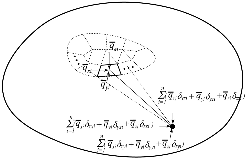
Equation (8) is the analytical solution under unit distribution force. According to the superposition principle of structural mechanics, the rheology deformation of any point on the surface of a soft soil foundation can be obtained. Figure 1 is the schematic diagram of the deformation of any point on the surface under distribution force. The soft soil foundation acts on the irregularly shaped distribution force. The rheology deformation of any time is calculated using the following steps:
- (1)
- The irregularly shaped region is dispersed into n little regions. The total time is dispersed into an l time step.
- (2)
- The irregularly shaped distribution force is dispersed into n distribution forces. The distribution forces in each region are shown as , , , where are the distribution forces in each region in the x direction; are the distribution forces in each region in the y direction; are the distribution forces in each region in the z direction.
- (3)
- The coordinate systems are set up. It takes each distributed load center point as the origin. The coordinates of the calculated position in each coordinate system are recorded as (x1,y1), (x2,y2),…, (xn,yn).
- (4)
- According to Equation (8), the deformation of each unit distribution load under each dispersed region is calculated.
- (5)
- The deformation of the calculated position on the surface under distribution force is shown as:where are the deformation of the position in the three directions; are the deformation of the calculated position in the x, y, and z directions under the first unit distribution force in the x direction; are the deformation of the calculated position in the x, y, and z directions under the first unit distribution force in the y direction; are the deformation of the calculated position in the x, y, and z directions under the first unit distribution force in the z direction; are the deformation of the calculated position in the x, y, and z directions under the nth unit distribution force in the x direction; are the deformation of the calculated position in the x, y, and z directions under the nth unit distribution force in the y direction; are the deformation of the calculated position in the x, y, and z directions under the nth unit distribution force in the z direction.
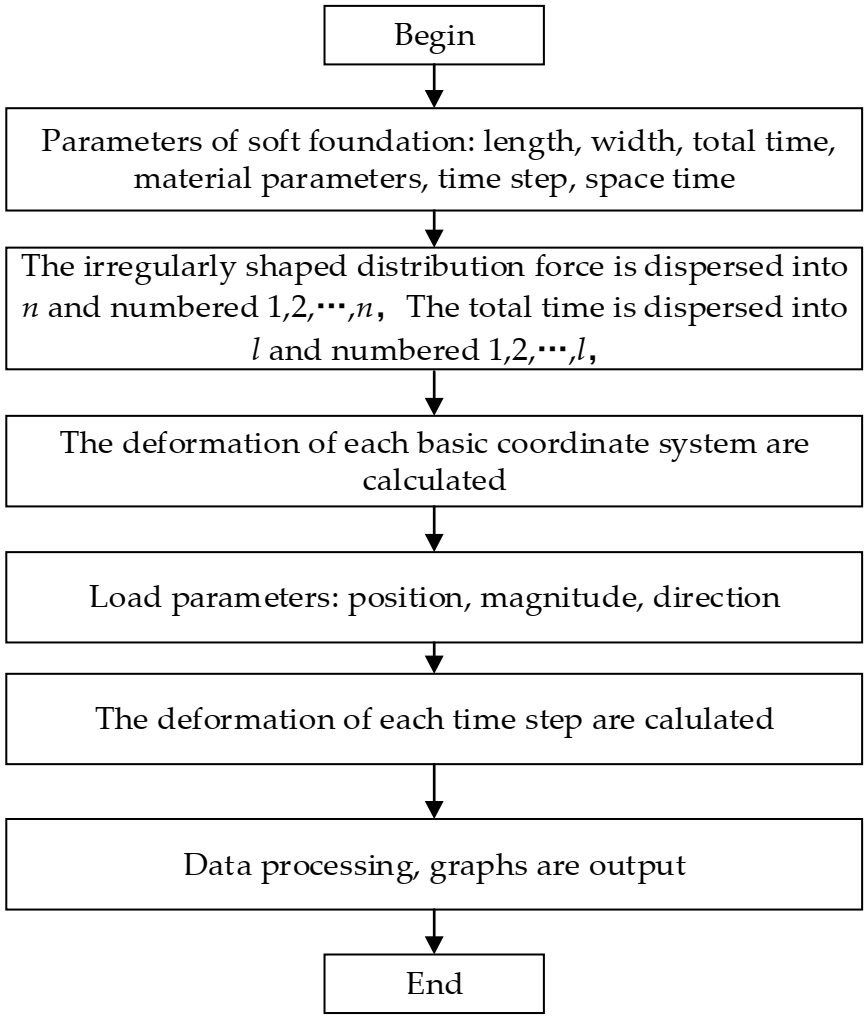
Figure 2 shows the flow chart of soft soil foundation surface deformation. The process mainly includes three parts: pre-processing, computational process, and post-processing. In pre-processing, the parameters of the soft soil foundation, the discretization of time, the discretization of forces, and the deformation of each basic coordinate system are calculated. In the computational process, the deformation of each time step is calculated. In post-processing, the results are processed into a graph.
4. The Parameter Inversion of Soft Soil Foundations
4.1. Quantum Genetic Algorithm
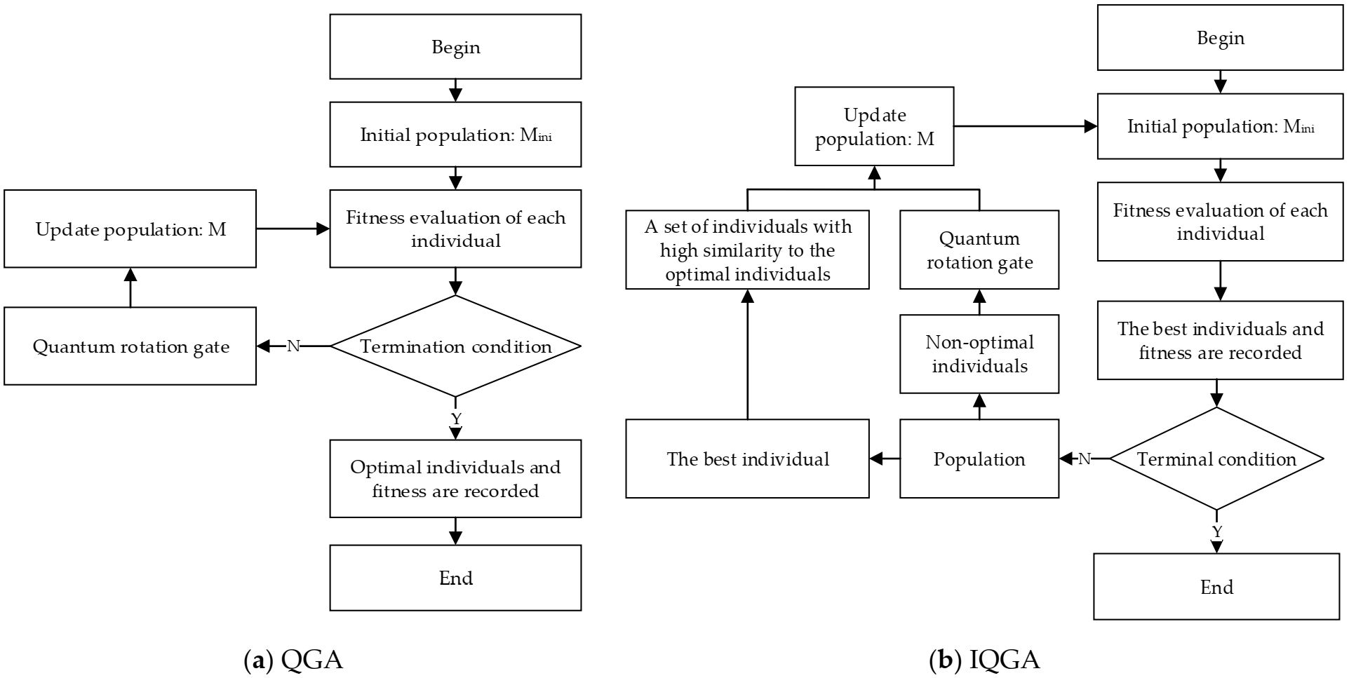
Inspired by the theory of quantum mechanics, Narayanan proposed a quantum genetic algorithm (QGA) in 1996. The QGA uses qubit coding instead of traditional chromosome coding. Therefore, it has a parallelism property and advantages in finding the global optimal solution.
The chromosome is shown by quantum states in the QGA method. A quantum state can be represented as the superposition of two states (0, 1). It is shown as:
where is a quantum state vector; are the probability of and , . Then, the individual qubit is shown as:
where are each quantum states of the individual qubit. The probability of an individual qubit is . A random number in the interval of [0, 1] can be used to assign binary 0s and 1s by comparing it with the probability of the quantum-bit when the chromosome is converted to a binary format.
The evolution of the population is completed by a quantum revolving gate. It is shown as:
where is the parameter of the rotation angle, ; is the direction of rotation; is the magnitude of the rotation angle.
4.2. Soft Soil Foundation Parameter Inversion Model
The rheology of soft soil foundations is a typical physical phenomenon. The deformation can be obtained by in-situ monitoring. The range of soft soil foundation parameters is shown as:
The initial parameters are . From Equations (8)–(10), the deformation of the monitoring positions are calculated. The optimal fitness for each generation is shown as:
where are the in-situ monitoring data. The termination conditions are shown as:
where is the termination value of the fitness value; is the maximum number of generations. If Equation (16) is not true, the quantum revolving gate is used for population evolution, and the fitness is calculated again until the termination conditions are met.
4.3. Improved Quantum Genetic Algorithm
In engineering projects, parameter inversion always needs to be calculated with a large amount of data. The QGA method has low computational efficiency in actual engineering calculations. It needs to be improved. The quantum genetic algorithm improves this in two ways. The algorithm processes of the QGA and IQGA are shown in Figure 3.
- (1)
- In each generation calculation, some individuals, similar to the optimal individuals of the previous generation, are formed so that individuals with certain guiding effects are produced in the next generation. The number of similar individuals, N, can be decided as shown:
- (2)
- The rotation angle is not a constant. The rotation angle is a big value when the number of generations is small. The rotation angle is a small value when the number of generations is big. It can be shown as:
Overall, computational efficiency can be accelerated in these theories by generating optimal individuals with high similarity and controlling the mutation process.
5. Case Study
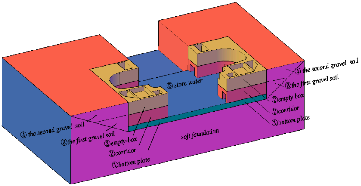
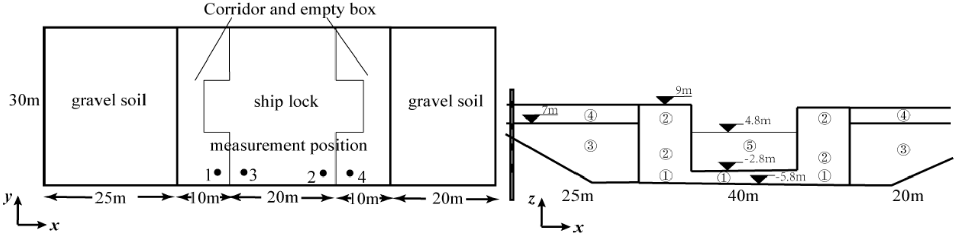
In hydraulic engineering, ship locks are always built on lakes and rivers. These foundations are mainly composed of clay and silt. Affected by the gravity of the structure, the uneven settlement of these soft soil foundations is serious. The monitoring data and construction processes of ship locks are shown in [34]. The ship lock diagram and construction processes are shown in Figure 4. The vertical view and side elevation of a ship lock and the measurement position are shown in Figure 5. The construction processes mainly contain: ① a bottom plate, ② a corridor and an empty box, ③ the first gravel, ④ the second gravel, and ⑤ store water. The length and width of gravel soil in the west are 25 and 30 m. The length and width of gravel soil in the east are 20 and 30 m. The length and width of the ship lock are 40 and 30 m. The bottom plate is finished on the 25th day. The first gravel soil is finished on the 125th day. The corridor and the empty box are finished on the 225th day. The second gravel soil is finished on the 250th day. The store water is finished on the 450th day. The water level is 6 m. The construction processes and simplified loading distribution are shown in Table 1. The density of plate, corridor, and empty box are 2400 kg/m3. The density of gravel soil is 1700 kg/m3. The density of store water is 1000 kg/m3. According to these materials’ densities, the gravity of each part is changed to the area loads.
The range of parameters is shown in Table 2.
The inversion parameters, using the QGA and IQGA methods, are shown as:
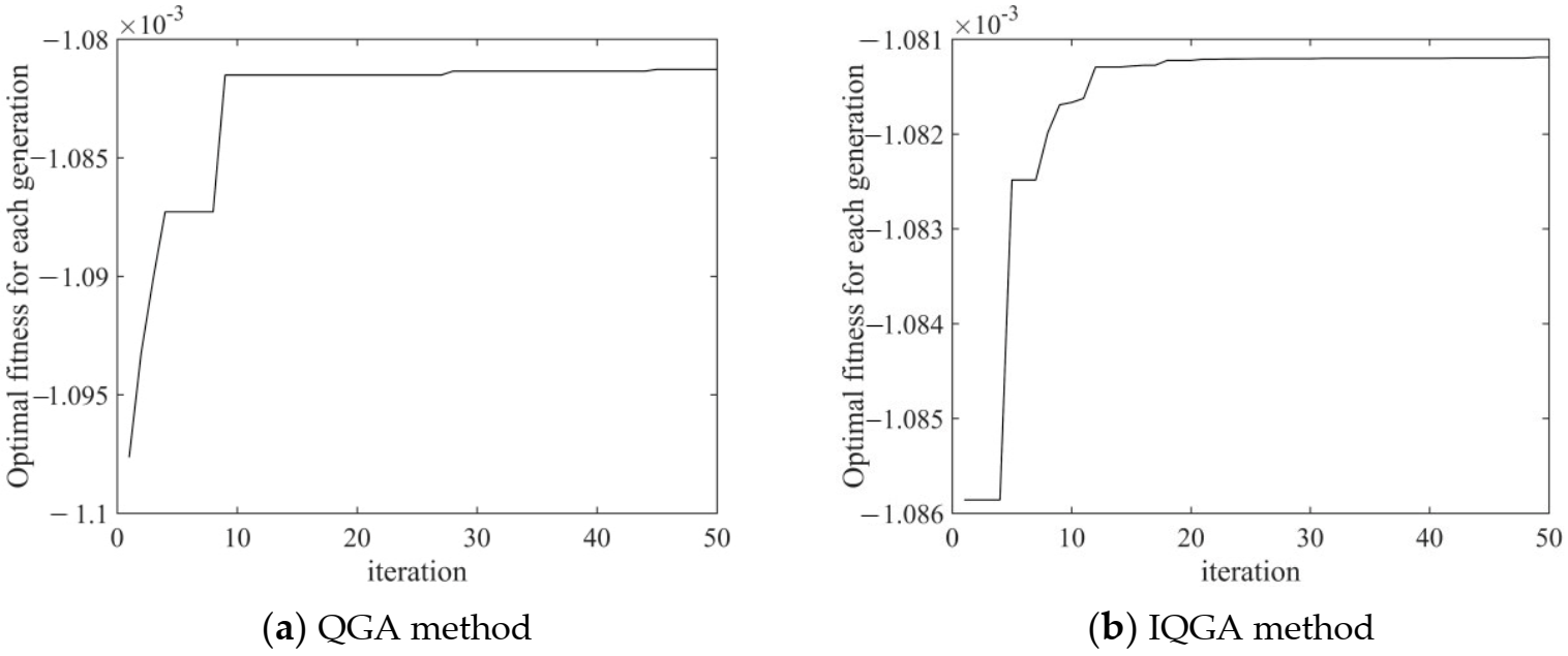
The inversion parameters of the two methods are similar and can be used as soft soil foundation parameters. Figure 6 is the convergence of the best fitness value for each generation. The figure shows that the optimal fitness value increases gradually with the increase in generations. The IQGA method converges to the optimal solution in the 20th generation. The QGA method converges to the optimal solution in the 40th generation. IQGA has faster convergence speed than QGA. The calculation efficiency is greatly improved.
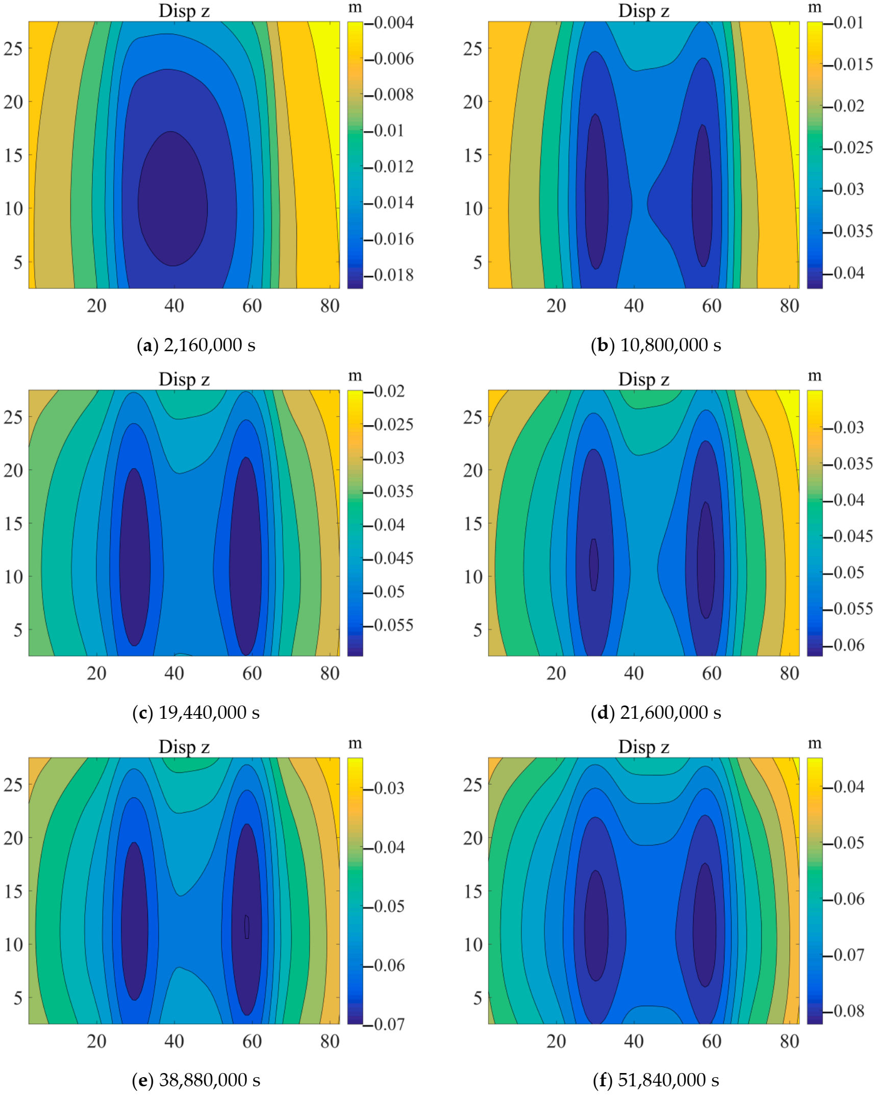
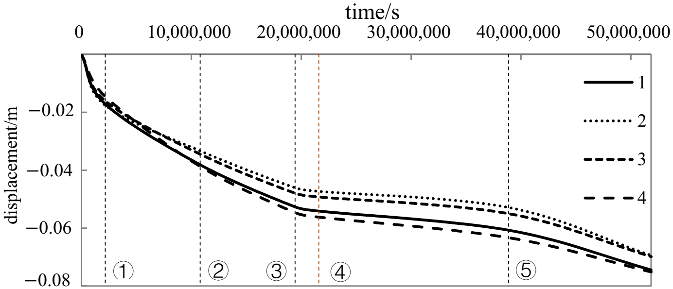
Table 3 shows the comparison between the measured values and calculated values of each position. It can be seen from the table that the calculated values at each location are in good agreement with the measured values. The parameters of the Maxwell viscoelastic soft soil foundation obtained by inversion in this paper are reliable. Figure 7 is the prediction displacement of the soft soil foundation in the z direction at each time. The gravity of gravel soil significantly changes the deformation distribution. The maximum deformation position is under the corridor. The creep of soil causes a 0.05–0.08 m settlement of the structure at 51,840,000 s. The displacement of each position in the z direction is shown in Figure 8. As the construction continues, the displacement of the foundation will increase rapidly after each process. At the end of calculation time, the displacement also has a tendency to increase. The measurement displacement can reach −0.075 m.
6. Conclusions
This paper reports a methodology to analyze the rheology of soft soil. Viscoelastic solutions under normal and tangential distributed force were obtained. The influence of construction sequences and loading was considered. An improved quantum genetic algorithm method was used to inverse the parameters of soft soil foundations. An engineering case was used to verify the accuracy of the method. The following important conclusions are summarized:
- (1)
- The viscoelastic solution of soft soil is based on calculus theory, Laplace integral transformation, and finite theory. The model is simple and has few parameters. The error between the predicted value and the measured value is acceptable.
- (2)
- The improved quantum genetic algorithm has a faster convergence speed than the quantum genetic algorithm. It is well applied to engineering.
- (3)
- The case shows that this method can be well appropriated for inversing the parameters of soft soil foundations and predicting the long-term uneven settlement deformation of buildings on soft soil foundations. It can be widely used in soft soil engineering.
Author Contributions
Conceptualization, H.Z. and C.S.; software, H.Z. and J.B.; writing—original draft preparation H.Z. and R.Y.; writing—review and editing, Y.M. and W.W.; All authors have read and agreed to the published version of the manuscript.
Funding
This work was funded by the National Natural Science Foundation of China (no. 51579089).
Institutional Review Board Statement
Not applicable.
Informed Consent Statement
Not applicable.
Data Availability Statement
Not applicable.
Conflicts of Interest
The authors declare no conflict of interest.
References
- Arora, K.R. Soil Mechanics and Foundation Engineering, 6th ed.; Lomus Offset Press: Delhi, India, 2006; pp. 587–635. [Google Scholar]
- Keedwell, M. Rheology and Soil Mechanics; Elsevier Applied Science: London, UK, 1984; pp. 67–69. [Google Scholar]
- Wang, R.; Xu, W.; Meng, Y.; Chen, H.; Zhou, Z. Numerical analysis of long-term stability of left bank abutment high slope at Jinping I hydropower station. Chin. J. Rock Mech. Eng. 2014, 33, 105–3113. [Google Scholar] [CrossRef]
- Barden, L. Consolidation of clay with non-linear viscosity. Geotechnique 1965, 15, 345–362. [Google Scholar] [CrossRef]
- Bjerrum, L. Engineering geology of Norwegian normally-consolidated marine clays as related to settlements of buildings. Geotechnique 1967, 17, 83–118. [Google Scholar] [CrossRef] [Green Version]
- Tjong-Kie, T. Determination of the rheological parameters and the hardening coefficients of Clays. In Rheology and Soil Mechanics/Rhéologie et Mécanique des Sols; Springer: Berlin/Heidelberg, Germany, 1966; pp. 256–272. [Google Scholar]
- Berre, T.; Iversen, K. Oedometer test with different specimen heights on a clay exhibiting large secondary compression. Geotechnique 1972, 22, 53–70. [Google Scholar] [CrossRef]
- Perzyna, P. Fundamental problems in viscoplasticity. Adv. Appl. Mech. 1966, 9, 243–377. [Google Scholar] [CrossRef]
- Su, C.; Zhang, H.; Hu, S.; Bai, J.; Dai, J. Combining Finite Element and Analytical methods to Contact Problems of 3D Structure on Soft Foundation. Math. Probl. Eng. 2020, 2020, 8827681. [Google Scholar] [CrossRef]
- Wang, L.; Wang, L. Semianalytical analysis of creep and thermal consolidation behaviors in layered saturated clays. Int. J. Geomech. 2020, 20, 06020001. [Google Scholar] [CrossRef]
- Borja, R.I. Generalized creep and stress relaxation model for clays. J. Geotech. Eng. 1992, 118, 1765–1786. [Google Scholar] [CrossRef]
- Yin, Z.Y.; Chang, C.S.; Karstunen, M.; Hicher, P.-Y. An anisotropic elastic–viscoplastic model for soft clays. Int. J. Solids Struct. 2010, 47, 665–677. [Google Scholar] [CrossRef] [Green Version]
- Alshamrani, M.A.; Sture, S. A time-dependent bounding surface model for anisotropic cohesive soils. Soils Found. 1998, 38, 61–76. [Google Scholar] [CrossRef] [Green Version]
- Adachi, T.; Oka, F.; Mimura, M. Mathematical structure of an overstress elasto-viscoplastic model for clay. Soils Found. 1987, 27, 31–42. [Google Scholar] [CrossRef] [Green Version]
- Singh, A.; Mitchell, J.K. General stress-strain-time function for soils. J. Soil Mech. Found. Div. 1968, 94, 21–46. [Google Scholar] [CrossRef]
- Ji, W.; Liu, X.; Qi, H.; Liu, X.; Lin, C.; Li, T. Mechanical Parameter Identification of Hydraulic Engineering with the Improved Deep Q-Network Algorithm. Math. Probl. Eng. 2020, 2020, 6404819. [Google Scholar] [CrossRef]
- Lin, C.; Li, T.; Chen, S.; Lin, C.; Liu, X.; Gao, L.; Sheng, T. Structural identification in long-term deformation characteristic of dam foundation using meta-heuristic optimization techniques. Adv. Eng. Softw. 2020, 148, 102870. [Google Scholar] [CrossRef]
- Chen, S.; Gu, C.; Lin, C.; Zhao, E.; Song, J. Safety monitoring model of a super-high concrete dam by using RBF neural network coupled with kernel principal component analysis. Math. Probl. Eng. 2018, 2018, 1712653. [Google Scholar] [CrossRef] [Green Version]
- Lin, C.; Li, T.; Chen, S.; Liu, X.; Lin, C.; Liang, S. Gaussian process regression-based forecasting model of dam deformation. Neural Comput. Appl. 2019, 31, 8503–8518. [Google Scholar] [CrossRef]
- Narayanan, A.; Moore, M. Quantum-inspired genetic algorithms. In Proceedings of the IEEE International Conference on Evolutionary Computation, Nagoya, Japan, 20–22 May 1996; pp. 61–66. [Google Scholar] [CrossRef]
- Grover, L.K. A fast quantum mechanical algorithm for database search. In Proceedings of the Twenty-Eighth Annual ACM Symposium on Theory of Computing, Philadelphia, PA, USA, 22–24 May 1996; Association for Computing Machinery: New York, NY, USA, 1996. [Google Scholar]
- Draa, A.; Meshoul, S.; Talbi, H.; Batouche, M. A quantum-inspired differential evolution algorithm for solving the N-queens problem. Neural Netw. 2011, 1, 21–27. [Google Scholar] [CrossRef] [Green Version]
- Ma, S.; Jin, W. A new parallel quantum genetic algorithm with probability-gate and its probability analysis. In Proceedings of the 2007 International Conference on Intelligent Systems and Knowledge Engineering, Chengdu, China, 15–16 October 2007; Atlantis Press: Paris, France, 2007. [Google Scholar] [CrossRef] [Green Version]
- Laboudi, Z.; Chikhi, S. Comparison of genetic algorithm and quantum genetic algorithm. Int. Arab J. Inf. Technol. 2012, 9, 243–249. [Google Scholar]
- Zhiber, A.V.; Startsev, S.Y. Integrals, solutions, and existence problems for Laplace transformations of linear hyperbolic systems. Math. Notes 2003, 74, 803–811. [Google Scholar] [CrossRef]
- Yüce, A.; Tan, N. On the approximate inverse Laplace transform of the transfer function with a single fractional order. Trans. Inst. Meas. Control 2021, 43, 1376–1384. [Google Scholar] [CrossRef]
- Ender, A.Y.; Énder, I.A.; Bakaleinikov, L.A.; Flegontova, E.Y. Construction of kernels of the nonlinear collision integral in the Boltzmann equation using laplace transformation. Tech. Phys. 2012, 57, 735–742. [Google Scholar] [CrossRef]
- Kim, Y.; Kim, B.M.; Jang, L.-C.; Kwon, J. A Note on Modified Degenerate Gamma and Laplace Transformation. Symmetry 2018, 10, 471. [Google Scholar] [CrossRef] [Green Version]
- Zhou, F.; Wang, L.; Liu, H. A fractional elasto-viscoplastic model for describing creep behavior of soft soil. Acta Geotech. 2021, 16, 67–76. [Google Scholar] [CrossRef]
- Varghese, V.; Bhoyar, S.; Khalsa, L. Thermoelastic response of a nonhomogeneous elliptic plate in the framework of fractional order theory. Arch. Appl. Mech. 2021, 91, 3223–3246. [Google Scholar] [CrossRef]
- Magdy, A.E. Analytical study of two-dimensional thermo-mechanical responses of viscoelastic skin tissue with temperature-dependent thermal conductivity and rheological properties. Mech. Based Des. Struct. Mach. 2021, 1–19. [Google Scholar] [CrossRef]
- Davis, R.; Selvadurai, A.; Pacheo, M. Elasticity and Geomechanics; Cambridge University Press: Cambridge, UK, 1998; p. 157. [Google Scholar]
- Chen, E.Y.; Pan, E.; Green, R. Surface loading of a multilayered viscoelastic pavement: Semianalytical solution. J. Eng. Mech. 2009, 135, 517–528. [Google Scholar] [CrossRef] [Green Version]
- Su, C.; Jiang, H.D.; Tan, E.H. An inverse analysis method for foundation parameters and its application based on viscoelastic foundation beam computation. Chin. J. Geotech. Eng. 2000, 22, 186–189. [Google Scholar]
Figure 1.
The schematic diagram of the deformation of any point on the surface under distribution force.
Figure 1.
The schematic diagram of the deformation of any point on the surface under distribution force.

Figure 2.
Flow chart of soft soil foundation surface deformation.

Figure 3.
The algorithm processes of QGA and IQGA.

Figure 4.
The ship lock diagram and construction processes.

Figure 5.
The vertical view and side elevation of the ship lock and the measurement position (descriptions of ①, ②, ③, ④, and ⑤ are shown in Figure 4).
Figure 5.
The vertical view and side elevation of the ship lock and the measurement position (descriptions of ①, ②, ③, ④, and ⑤ are shown in Figure 4).

Figure 6.
Convergence of the optimal fitness for each generation.

Figure 7.
The prediction displacement of the soft soil foundation in the z direction at each time.

Figure 8.
The displacement of each position in the z direction (descriptions of ①, ②, ③, ④ and ⑤ are shown in Figure 4).
Figure 8.
The displacement of each position in the z direction (descriptions of ①, ②, ③, ④ and ⑤ are shown in Figure 4).


Table 1.
The construction processes and simplified loading distribution.
| Construction Processes | Time | Loads | ||||
|---|---|---|---|---|---|---|
| Backfill in West (N/m2) | Bottom Plate in West (N/m2) | Middle Plate (N/m2) | Bottom Plate in East (N/m2) | Backfill in East (N/m2) | ||
| ① Bottom plate | 2,160,000 s | 0 | 72,000 | 72,000 | 72,000 | 0 |
| ② Corridor and empty-box | 10,800,000 s | 0 | 236,000 | 72,000 | 200,000 | 0 |
| ③ First gravel | 19,440,000 s | 68,000 | 236,000 | 72,000 | 200,000 | 68,000 |
| ④ Second gravel | 21,600,000 s | 102,000 | 236,000 | 72,000 | 200,000 | 102,000 |
| ⑤ Store water | 38,880,000 s | 102,000 | 236,000 | 132,000 | 200,000 | 102,000 |
Table 2.
The range of parameters.
| Parameters | Range |
|---|---|
| 0.15 ~ 0.40 | |
| Population size | 40 |
| Maximum generation | 50 |
Table 3.
The comparison of calculated values and measured values (unit: m).
| Position | Data | Time | |||||
|---|---|---|---|---|---|---|---|
| 2,160,000 s | 10,800,000 s | 19,440,000 s | 21,600,000 s | 38,880,000 s | 51,840,000 s | ||
| 1 | Measured | −0.0192 | −0.0399 | −0.0542 | −0.0548 | −0.0609 | −0.0721 |
| QGA | −0.0171 | −0.0381 | −0.0527 | −0.0541 | −0.0607 | −0.0744 | |
| IQGA | −0.0169 | −0.0378 | −0.0526 | −0.0541 | −0.0608 | −0.0744 | |
| 2 | Measured | −0.0191 | −0.0378 | −0.0619 | −0.0631 | −0.0793 | −0.0850 |
| QGA | −0.0176 | −0.0333 | −0.0461 | −0.0473 | −0.0529 | −0.0694 | |
| IQGA | −0.0173 | −0.0331 | −0.0461 | −0.0473 | −0.0530 | −0.0694 | |
| 3 | Measured | −0.0173 | −0.0302 | −0.0404 | −0.0400 | −0.0467 | −0.0599 |
| QGA | −0.0161 | −0.0345 | −0.0479 | −0.0492 | −0.0550 | −0.0698 | |
| IQGA | −0.0160 | −0.0343 | −0.0479 | −0.0492 | −0.0550 | −0.0699 | |
| 4 | Measured | −0.0177 | −0.0314 | −0.0430 | −0.0435 | −0.0589 | −0.0638 |
| QGA | −0.0145 | −0.0387 | −0.0546 | −0.0562 | −0.0633 | −0.0751 | |
| IQGA | −0.0145 | −0.0386 | −0.0547 | −0.0563 | −0.0635 | −0.0754 | |
Publisher’s Note: MDPI stays neutral with regard to jurisdictional claims in published maps and institutional affiliations. |
© 2021 by the authors. Licensee MDPI, Basel, Switzerland. This article is an open access article distributed under the terms and conditions of the Creative Commons Attribution (CC BY) license (https://creativecommons.org/licenses/by/4.0/).
Share and Cite
MDPI and ACS Style
Zhang, H.; Su, C.; Bai, J.; Yuan, R.; Ma, Y.; Wang, W. The Rheological Analytical Solution and Parameter Inversion of Soft Soil Foundation. Symmetry 2021, 13, 1228. https://0-doi-org.brum.beds.ac.uk/10.3390/sym13071228
AMA Style
Zhang H, Su C, Bai J, Yuan R, Ma Y, Wang W. The Rheological Analytical Solution and Parameter Inversion of Soft Soil Foundation. Symmetry. 2021; 13(7):1228. https://0-doi-org.brum.beds.ac.uk/10.3390/sym13071228
Chicago/Turabian StyleZhang, Heng, Chao Su, Jiawei Bai, Rongyao Yuan, Yujun Ma, and Wenjun Wang. 2021. "The Rheological Analytical Solution and Parameter Inversion of Soft Soil Foundation" Symmetry 13, no. 7: 1228. https://0-doi-org.brum.beds.ac.uk/10.3390/sym13071228
Note that from the first issue of 2016, this journal uses article numbers instead of page numbers. See further details here.