Morphology of an Interacting Three-Dimensional Trapped Bose–Einstein Condensate from Many-Particle Variance Anisotropy

Abstract

The variance of the position operator is associated with how wide or narrow a wave-packet is, the momentum variance is similarly correlated with the size of a wave-packet in momentum space, and the angular-momentum variance quantifies to what extent a wave-packet is non-spherically symmetric. We examine an interacting three-dimensional trapped Bose–Einstein condensate at the limit of an infinite number of particles, and investigate its position, momentum, and angular-momentum anisotropies. Computing the variances of the three Cartesian components of the position, momentum, and angular-momentum operators we present simple scenarios where the anisotropy of a Bose–Einstein condensate is different at the many-body and mean-field levels of theory, despite having the same many-body and mean-field densities per particle. This suggests a way to classify correlations via the morphology of 100% condensed bosons in a three-dimensional trap at the limit of an infinite number of particles. Implications are briefly discussed.

1. Introduction

There has been an increasing interest in the theory and properties of trapped Bose–Einstein condensates at the limit of an infinite number of particles [1,2,3,4,5,6,7,8,9,10,11,12]. Here, one may divide the research questions into two, inter-connected groups. The first group of research questions deals with rigorous results, mainly proving when many-body and mean-field, Gross–Pitaevskii theories coincide at this limit, whereas the second group of questions deals with characterizing correlations in a trapped Bose–Einstein condensate based on the difference between many-body and mean-field properties at the infinite-particle-number limit. In [2], it has been shown that the ground-state energy per particle and density per particle computed at the many-body level of theory coincide with the respective mean-field results. The infinite-particle-number limit is defined such that the interaction parameter, i.e., the product of the number of bosons times the interaction strength (proportional to the scattering length), is held constant. Similarly, in [3] it has been shown that the reduced one-body and any reduced finite-n-body density matrix [13,14] per particle are 100% condensed, and that the leading natural orbital boils down to the Gross–Pitaevskii single-particle function. Analogous results connecting time-dependent many-body and mean-field theories are given in [4,5] and developments for mixtures in [9,10,11]. In [12], the many-boson wave-function at the infinite-particle-number limit has been constructed explicitly.

The difference between many-body and mean-field theories at the limit of an infinite number of particles, which as stated above coincide at the level of the energy, densities, and reduced density matrices per particle, starts to show up in variances of many-particle observables [6,7]. Of course, the wave-functions themselves differ and their overlap is smaller than one [8]. In evaluating the variances of many-particle observables two-body operators emerge whose combination with the elements of the reduced two-body density matrix can pick up even the tiniest depletion, which always exist due to the inter-particle interaction [6,7]. Here, the quantitative difference between the many-body and mean-field variances is a useful tool to benchmark many-body numerical approaches [15,16], whereas the qualitative differences serve to define and characterize the nature of correlations in 100% condensed bosons at the infinite-particle-number limit.

Qualitative differences between the many-body and mean-field variances per particle depend on both the system and observable under investigation and emerge because the 100% condensed bosons are interacting. In the ground-state of a one-dimensional double-well potential, the mean-field position variance per particle increases monotonously with the interaction parameter whereas, once about a single particle is excited outside the condensed mode, the many-body position variance per particle starts to decrease [6]. In the analogous time-dependent setup of a bosonic Josephson junction, the mean-field variance is oscillating and bound by the size of the junction, whereas the many-body variance increases to ‘sizes’ several times larger [7]. In two spatial dimensions additional features come out. The position variance per particle in a thin annulus can exhibit a different dimensionality [17] and both the position and momentum variances can exhibit opposite anisotropies [18] when computed at the many-body and mean-field levels of theory in an out-of-equilibrium quench dynamics. In two spatial dimensions the many-particle variance of the ${\widehat{L}}_Z$ component of the angular-momentum operator becomes available, and used to analyze the lack of conservation of symmetries in the mean-field dynamics [19].

In the present work we analyze the many-particle position, momentum, and angular-momentum variances of a three-dimensional anisotropic trapped Bose–Einstein condensate at the limit of an infinite number of particles, focusing on three-dimensional scenarios that do not have (one-dimensional and) two-dimensional analogs. Mainly, the available permutations between the three Cartesian components of a many-particle operator, such as the position and momentum operators, allow one for various different anisotropies of the respective mean-field and many-body variances than in two spatial dimensions [18]. Furthermore, anisotropy of the angular-momentum variance can only be investigated when there is more than one component, and this occurs with the three Cartesian components of the angular-momentum operator in three spatial dimensions.

The structure of the paper is as follows. In Section 2 theory and definitions are developed. In Section 3 we present two applications where a common methodological line of investigation is that the variances at the many-body level of theory can be computed analytically. In Section 3.1, the anisotropy of the position and momentum variances in the out-of-equilibrium breathing dynamics of a Bose–Einstein condensate in a three-dimensional anisotropic harmonic potential are analyzed, and in Section 3.2, a solvable model is devised which allows one to analyze the anisotropy of the angular-momentum variances in the ground state of interacting bosons in a three-dimensional anisotropic harmonic potential. All quantities are computed at the infinite-particle-number limit. Finally, we summarize in Section 4.

2. Theory

The variances per particle of a many-particle observable $\widehat{O}={\sum }_{j=1}^N{\widehat{o}}_j$ computed at the many-body (MB) and mean-field, Gross–Pitaevskii (GP) levels of theory are connected at the limit of an infinite number of particles by the following relation [6]:

$${\mathrm{Var}|}_{\mathrm{MB}}(\widehat{O})={\mathrm{Var}|}_{\mathrm{GP}}(\widehat{O})+{\mathrm{Var}|}_{\mathrm{correlations}}(\widehat{O}).$$

(1)

Here, ${\mathrm{Var}|}_{\mathrm{MB}}(\widehat{O})={lim}_{N\to \infty }\left[\frac{1}{N}(\langle \Psi |{\widehat{O}}^2|\Psi \rangle -\langle \Psi |\widehat{O}{|\Psi \rangle }^2)\right]$, where $\Psi$ is the solution of the many-particle Schrödinger equation, and ${\mathrm{Var}|}_{\mathrm{GP}}(\widehat{O})=\langle {\psi }_{GP}|{\widehat{o}}^2|{\psi }_{GP}\rangle -\langle {\psi }_{GP}|\widehat{o}{|{\psi }_{GP}\rangle }^2$, where ${\psi }_{GP}$ is the solution of the corresponding Gross–Pitaevskii equation. Recall that the infinite-particle-number limit is defined such that the interaction parameter, i.e., the product of the number of bosons times the interaction strength, is kept fixed. Furthermore, only in the infinite-particle-number limit the density per particle is identical at the many-body and mean-field levels of theory, and thus (1) compares the variances per particle of the same density per particle. The correlations term, ${\mathrm{Var}|}_{\mathrm{correlations}}(\widehat{O})$, quantifying the difference between the mean-field and many-body variances, depends on the elements of the reduced two-body density matrix where at least one of the indexes corresponds to a natural orbital higher than the condensed mode [6]. For non-interacting bosons the correlations term obviously vanishes. As stated above, one is interested in qualitative differences between ${\mathrm{Var}|}_{\mathrm{GP}}(\widehat{O})$ and ${\mathrm{Var}|}_{\mathrm{MB}}(\widehat{O})$ and their origin.

Consider a Bose–Einstein condensate for which the many-body variances of the three Cartesian components of, say, the position operator are different and satisfy, without loss of generality, the anisotropy

$${\mathrm{Var}|}_{\mathrm{MB}}(\widehat{X})>{\mathrm{Var}|}_{\mathrm{MB}}(\widehat{Y})>{\mathrm{Var}|}_{\mathrm{MB}}(\widehat{Z}).$$

(2a)

We define the following classification with respect to the possible different anisotropies of the respective mean-field position variances:

$$\begin{array}{ccc}\hfill \left\{1\right\}:& & \left\{{\mathrm{Var}|}_{\mathrm{GP}}(\widehat{X})>{\mathrm{Var}|}_{\mathrm{GP}}(\widehat{Y})>{\mathrm{Var}|}_{\mathrm{GP}}(\widehat{Z})\right\},\hfill \\ \hfill \{1,2\}:& & \{{\mathrm{Var}|}_{\mathrm{GP}}(\widehat{Y})>{\mathrm{Var}|}_{\mathrm{GP}}(\widehat{X})>{\mathrm{Var}|}_{\mathrm{GP}}(\widehat{Z});\hfill \\ \hfill & & {\mathrm{Var}|}_{\mathrm{GP}}(\widehat{X})>{\mathrm{Var}|}_{\mathrm{GP}}(\widehat{Z})>{\mathrm{Var}|}_{\mathrm{GP}}(\widehat{Y});\hfill \\ \hfill & & {\mathrm{Var}|}_{\mathrm{GP}}(\widehat{Z})>{\mathrm{Var}|}_{\mathrm{GP}}(\widehat{Y})>{\mathrm{Var}|}_{\mathrm{GP}}(\widehat{X})\},\hfill \\ \hfill \{1,2,3\}:& & \{{\mathrm{Var}|}_{\mathrm{GP}}(\widehat{Y})>{\mathrm{Var}|}_{\mathrm{GP}}(\widehat{Z})>{\mathrm{Var}|}_{\mathrm{GP}}(\widehat{X});\hfill \\ \hfill & & {\mathrm{Var}|}_{\mathrm{GP}}(\widehat{Z})>{\mathrm{Var}|}_{\mathrm{GP}}(\widehat{X})>{\mathrm{Var}|}_{\mathrm{GP}}(\widehat{Y})\}.\hfill \end{array}$$

(2b)

Naturally, the classification (2b) follows the classes of the $S_3$ permutation group denoted by $\left\{1\right\}$, $\{1,2\}$, and $\{1,2,3\}$. If the mean-field variances exhibit anisotropy other than the anisotropy of the respective many-body variances, i.e., the ordering of the former does not belong to the class $\left\{1\right\}$, we may interpret that the mean-field and many-body morphologies of the Bose–Einstein condensate with respect to the operators under investigation are distinct. This implies that the correlations term in (1) becomes dominate for the variances of these operators. In the present work we investigate manifestations of definition (2) utilizing the many-particle position ($\widehat{X},\widehat{Y},\widehat{Z}$), momentum (${\widehat{P}}_X,{\widehat{P}}_Y,{\widehat{P}}_Z$), and angular-momentum (${\widehat{L}}_X,{\widehat{L}}_Y,{\widehat{L}}_Z$) operators for classifying the morphology of 100% condensed trapped bosons at the limit of an infinite number of particles.

3. Applications

3.1. Position and Momentum Variances in an Out-of-Equilibrium Dynamics of a Three-Dimensional Trapped Bose–Einstein Condensate

Consider N structureless bosons trapped in a three-dimensional anisotropic harmonic potential and interacting by a general two-body interaction $\widehat{W}(\mathbf{r}-{\mathbf{r}}^{\prime })$. The frequencies of the trap satisfy, without loss of generality, ${\omega }_x<{\omega }_y<{\omega }_z$. We work with dimensionless quantities, $\hslash =m=1$. Using Jacobi coordinates, ${\mathbf{Q}}_k=\frac{1}{\sqrt{k(k+1)}}{\sum }_{j=1}^k({\mathbf{r}}_{k+1}-{\mathbf{r}}_j),k=1,\dots ,N-1$, ${\mathbf{Q}}_N=\frac{1}{\sqrt{N}}{\sum }_{j=1}^N{\mathbf{r}}_j$, where ${\mathbf{r}}_1,\dots ,{\mathbf{r}}_N$ are the coordinates in the laboratory frame, the Hamiltonian can be written as:

$$\begin{array}{c}\hfill \widehat{H}({\mathbf{Q}}_1,\dots ,{\mathbf{Q}}_N)=-\frac{1}{2}\frac{{\partial }^2}{\partial {\mathbf{Q}}_N^2}+\frac{1}{2}\left({\omega }_x^2{Q}_{N,x}^2+{\omega }_y^2{Q}_{N,y}^2+{\omega }_z^2{Q}_{N,z}^2\right)+{\widehat{H}}_{rel}({\mathbf{Q}}_1,\dots ,{\mathbf{Q}}_{N-1}).\end{array}$$

(3)

The ‘relative’ Hamiltonian ${\widehat{H}}_{rel}$ collects all terms depending on the relative coordinates ${\mathbf{Q}}_1,\dots ,{\mathbf{Q}}_{N-1}$, and ${\mathbf{Q}}_k=(Q_{k,x},Q_{k,y},Q_{k,z})$. Suppose now that the bosons are prepared in the ground state of the non-interacting system. The ground-state is separable in the Jacoby coordinates and reads $\mathsf{\Phi }({\mathbf{Q}}_1,\dots ,{\mathbf{Q}}_N)={\left(\frac{{\omega }_x}{\pi }\right)}^{\frac{N}{4}}{\left(\frac{{\omega }_y}{\pi }\right)}^{\frac{N}{4}}{\left(\frac{{\omega }_z}{\pi }\right)}^{\frac{N}{4}}{e}^{-\frac{1}{2}{\sum }_{k=1}^N\left({\omega }_x{Q}_{k,x}^2+{\omega }_y{Q}_{k,y}^2+{\omega }_z{Q}_{k,z}^2\right)}$, where the relation ${\sum }_{j=1}^N{\mathbf{r}}_j^2={\sum }_{k=1}^N{\mathbf{Q}}_k^2$ connecting the laboratory and Jacoby coordinates is used. The solution of the time-dependent many-boson Schrödinger equation, $\widehat{H}\Psi (t)=i\frac{\partial \Psi (t)}{\partial t}$, where $\Phi$ is the initial condition, reads $\Psi (t)=e^{-i\widehat{H}t}\Phi$. Consequently, because of the center-of-mass separability of the Hamiltonian $\widehat{H}$ and of $\Phi$, the position and momentum variances per particle of the time-dependent state $\Psi (t)$, for a general inter-particle interaction $\widehat{W}(\mathbf{r}-{\mathbf{r}}^{\prime })$, are those of the static, non-interacting system:

$$\begin{array}{ccc}\hfill & & {\mathrm{Var}|}_{\mathrm{MB}}(\widehat{X})=\frac{1}{2{\omega }_x},{\mathrm{Var}|}_{\mathrm{MB}}(\widehat{Y})=\frac{1}{2{\omega }_y},{\mathrm{Var}|}_{\mathrm{MB}}(\widehat{Z})=\frac{1}{2{\omega }_z},\hfill \\ & & {\mathrm{Var}|}_{\mathrm{MB}}({\widehat{P}}_X)=\frac{{\omega }_x}{2},{\mathrm{Var}|}_{\mathrm{MB}}({\widehat{P}}_Y)=\frac{{\omega }_y}{2},{\mathrm{Var}|}_{\mathrm{MB}}({\widehat{P}}_Z)=\frac{{\omega }_z}{2}.\hfill \end{array}$$

(4)

In other words, the anisotropies ${\mathrm{Var}|}_{\mathrm{MB}}(\widehat{X})>{\mathrm{Var}|}_{\mathrm{MB}}(\widehat{Y})>{\mathrm{Var}|}_{\mathrm{MB}}(\widehat{Z})$ of the position operator and ${\mathrm{Var}|}_{\mathrm{MB}}({\widehat{P}}_Z)>{\mathrm{Var}|}_{\mathrm{MB}}({\widehat{P}}_Y)>{\mathrm{Var}|}_{\mathrm{MB}}({\widehat{P}}_X)$ of the momentum operator, when computed at the many-body level of theory, hold for all times during the out-of-equilibrium dynamics, see the constant-value (dashed) curves in Figure 1 and Figure 2. We note that the variances per particle (4) hold for any number of bosons due to the separability of the center-of-mass. However, only at the limit of an infinite number of particles the density per particle coincides within many-body and mean-field levels of theory and can thus be exactly computed from the Gross–Pitaevskii equation.

What happens at the Gross–Pitaevskii level of theory? Can the mean-field variances have different orderings than the many-body variances, i.e., belong to other anisotropy classes based on the $S_3$ permutation group, see (2b), than to $\left\{1\right\}$? If yes, then why and how? The Gross–Pitaevskii or non-linear Schrödinger equation is given by $\left[-\frac{1}{2}\frac{{\partial }^2}{\partial {\mathbf{r}}^2}+\frac{1}{2}\left({\omega }_x^2{x}^2+{\omega }_y^2{y}^2+{\omega }_z^2{z}^2\right)+g{\left|{\psi }_{GP}(\mathbf{r},t)\right|}^2\right]{\psi }_{GP}(\mathbf{r},t)=i\frac{\partial {\psi }_{GP}(\mathbf{r},t)}{\partial t}$, where $g=4\pi N{a}_s$ is the coupling constant and $a_s$ the s-wave scattering length of the above two-body interaction $\widehat{W}(\mathbf{r}-{\mathbf{r}}^{\prime })$. The initial condition, as above, is the ground state of the non-interacting system, ${\psi }_{GP}(\mathbf{r},0)={\left(\frac{{\omega }_x}{\pi }\right)}^{\frac{1}{4}}{\left(\frac{{\omega }_y}{\pi }\right)}^{\frac{1}{4}}{\left(\frac{{\omega }_z}{\pi }\right)}^{\frac{1}{4}}{e}^{-\frac{1}{2}\left({\omega }_x{x}^2+{\omega }_y{y}^2+{\omega }_z{z}^2\right)}$. The Gross–Pitaevskii equation does not maintain the center-of-mass separability of the initial condition because of its non-linear term, which, therefore, can lead to variations of the position and momentum variances when computed at the mean-field level of theory.

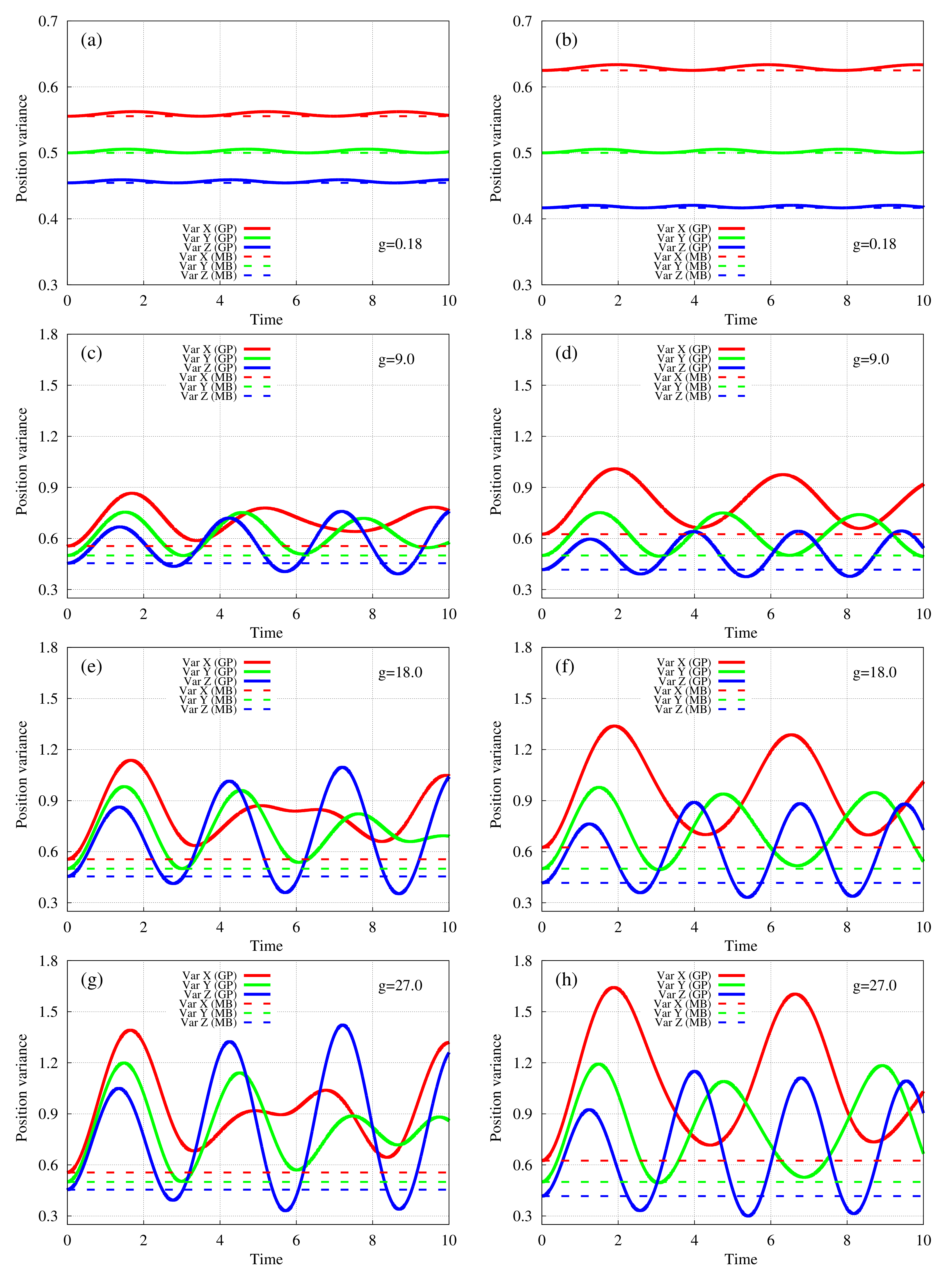
Figure 1 and Figure 2 display the Gross–Pitaevskii dynamics of the position and momentum variances per particle, respectively, for four coupling constants, $g=0.18,9.0,18.0$, and $27.0$. To integrate the three-dimensional Gross–Pitaevskii equation we use a box of size $[-10,10)\times [-10,10)\times [-10,10)$, a Fourier-discrete-variable-representation with ${128}^3$ grid points and periodic boundary conditions, and the numerical implementation embedded in [20]. The dynamics are computed for the four coupling constants g and depicted by the oscillating (solid) curves in Figure 1 and Figure 2. The left columns are for a 10% anisotropy of the harmonic trap, i.e., ${\omega }_x=0.9$, ${\omega }_y=1.0$, and ${\omega }_z=1.1$, and the right columns are for a 20% anisotropy of the harmonic trap, namely, ${\omega }_x=0.8$, ${\omega }_y=1.0$, and ${\omega }_z=1.2$. We remark that the expectation values per particle of the position ($\widehat{X},\widehat{Y},\widehat{Z}$) and momentum (${\widehat{P}}_X,{\widehat{P}}_Y,{\widehat{P}}_Z$) operators computed at the mean-field and many-body levels of theory coincide at the limit of an infinite number of particles and are all equal to zero in the present scenario.

For the smallest coupling constant, $g=0.18$, we see that the mean-field variances oscillate with very small amplitudes around the respective constant values of the many-body variances. This means that the mean-field anisotropy of the position variance, ${\mathrm{Var}|}_{\mathrm{GP}}(\widehat{X})>{\mathrm{Var}|}_{\mathrm{GP}}(\widehat{Y})>{\mathrm{Var}|}_{\mathrm{GP}}(\widehat{Z})$, and its many-body anisotropy, ${\mathrm{Var}|}_{\mathrm{MB}}(\widehat{X})>{\mathrm{Var}|}_{\mathrm{MB}}(\widehat{Y})>{\mathrm{Var}|}_{\mathrm{MB}}(\widehat{Z})$, are alike. A similar situation is found for the momentum variance, namely, that the mean-field momentum anisotropy, ${\mathrm{Var}|}_{\mathrm{GP}}({\widehat{P}}_Z)>{\mathrm{Var}|}_{\mathrm{GP}}({\widehat{P}}_Y)>{\mathrm{Var}|}_{\mathrm{GP}}({\widehat{P}}_X)$, and the many-body anisotropy, ${\mathrm{Var}|}_{\mathrm{MB}}({\widehat{P}}_Z)>{\mathrm{Var}|}_{\mathrm{MB}}({\widehat{P}}_Y)>{\mathrm{Var}|}_{\mathrm{MB}}({\widehat{P}}_X)$, are the same. Consequently, we may conclude that for small coupling constants the anisotropy class of the position operator is $\left\{1\right\}$ and, likewise, the anisotropy class of the momentum operator is $\left\{1\right\}$, see (2). In other words, the contribution of the correlations term in (1) is marginal.

The situation becomes more interesting for the larger coupling constants, $g=9.0,18.0$, and $27.0$. We begin with the position variances, Figure 1. The variances are found to oscillate prominently, with much larger amplitudes than for $g=0.18$, and, subsequently, to cross each other. There are three ingredients that enable and govern this crossing dynamics. The first, is that the amplitudes of oscillations of ${\mathrm{Var}|}_{\mathrm{GP}}(\widehat{X})$, ${\mathrm{Var}|}_{\mathrm{GP}}(\widehat{Y})$, and ${\mathrm{Var}|}_{\mathrm{GP}}(\widehat{Z})$ are slightly different already at short times, with the former being the larger and the latter being the smaller (more prominent for 20% than for 10% trap anisotropy). The second, is that the respective frequencies of oscillations are also slightly different at short times, with the former being the smaller and the latter being the larger. Both features correlate with the ordering of the frequencies of the trap, ${\omega }_x<{\omega }_y<{\omega }_z$. The third ingredient is that the three Cartesian components are coupled to each other during the dynamics, what impacts the oscillatory pattern at intermediate and later times (more prominent for 10% than for 20% trap anisotropy, see Figure 1).

Combing the above, we find for the 10% trap anisotropy that around $t=4.0$ ${\mathrm{Var}|}_{\mathrm{GP}}(\widehat{Z})>{\mathrm{Var}|}_{\mathrm{GP}}(\widehat{Y})>{\mathrm{Var}|}_{\mathrm{GP}}(\widehat{X})$ takes place, around $t=6.0$ ${\mathrm{Var}|}_{\mathrm{GP}}(\widehat{X})>{\mathrm{Var}|}_{\mathrm{GP}}(\widehat{Y})>{\mathrm{Var}|}_{\mathrm{GP}}(\widehat{Z})$ holds (again), and around $t=7.0$ ${\mathrm{Var}|}_{\mathrm{GP}}(\widehat{Z})>{\mathrm{Var}|}_{\mathrm{GP}}(\widehat{Y})>{\mathrm{Var}|}_{\mathrm{GP}}(\widehat{X})$ occurs. In other words, the anisotropy class of the position variance starts as $\left\{1\right\}$ for $t=0$, changes to $\{1,2\}$ around $t=4$, is back to $\left\{1\right\}$ around $t=6$, and becomes $\{1,2,3\}$ around $t=7$. Furthermore, this pattern is found to be robust for different, increasing coupling constants, see Figure 1. For 20% trap anisotropy we find a different crossing patten of the position variances. The anisotropy class begins as $\left\{1\right\}$ for $t=0$, changes at around $t=3.0$ to $\{1,2\}$, and immediately after, at around $t=3.75$, it is $\{1,2,3\}$. Now, around $t=7.0$ there is a broad regime of anisotropy class $\{1,2\}$. Another difference of a geometrical origin between the dynamics in the 20% and 10% trap anisotropies can be seen for $g=9$, see Figure 1c,d. Here, the coupling constant is sufficiently large to lead to crossing of all position variances for the 10% anisotropy trap, and, consequently, to the position anisotropy class $\{1,2,3\}$ (at around $t=7$). On the other hand, for the 20% anisotropy trap the coupling constant is just short of allowing all position variances to cross each other and, clearly, the anisotropy class $\{1,2,3\}$ cannot occur (as it happens at around $t=3.75$ for the further larger coupling constants, $g=18$ and 27). All in all, we have demonstrated in a rather common (out-of-equilibrium quench) scenario the emergence of anisotropy classes other than $\left\{1\right\}$, i.e., $\{1,2\}$ and $\{1,2,3\}$, for the position operator of a Bose–Einstein condensate at the infinite-particle-number limit. Hence, the correlations term in (1) for the position variance becomes dominant in the dynamics.

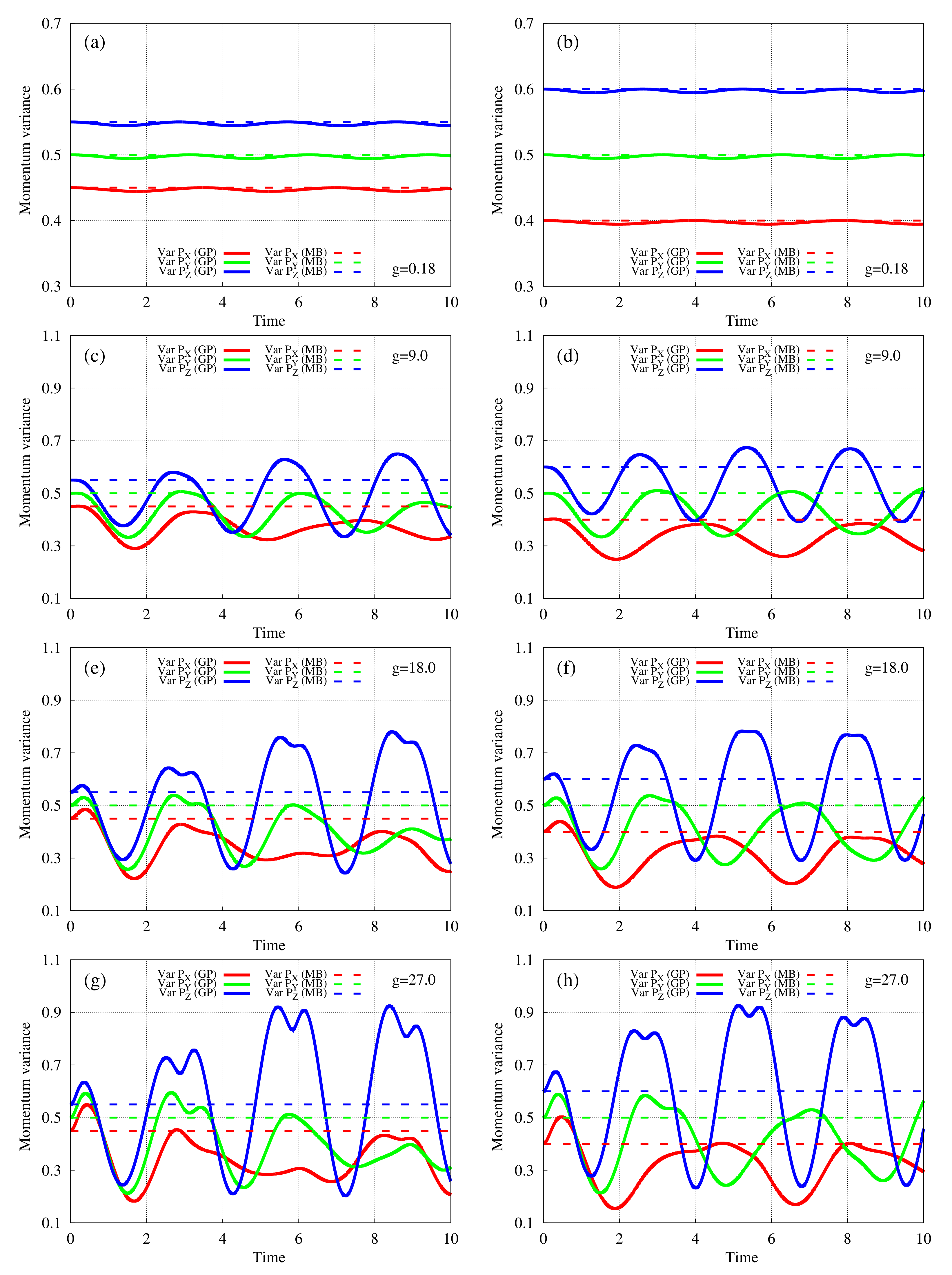
The results for the momentum variances per particle, see Figure 2, follow similar and corresponding trends as those for the position operator, albeit the crossings of the respective momentum curves take place during slightly narrower time windows than for the position operator for the parameters used. Thus, for the 10% trap anisotropy we have ${\mathrm{Var}|}_{\mathrm{GP}}({\widehat{P}}_X)>{\mathrm{Var}|}_{\mathrm{GP}}({\widehat{P}}_Y)>{\mathrm{Var}|}_{\mathrm{GP}}({\widehat{P}}_Z)$ around $t=4.25$, ${\mathrm{Var}|}_{\mathrm{GP}}({\widehat{P}}_Z)>{\mathrm{Var}|}_{\mathrm{GP}}({\widehat{P}}_Y)>{\mathrm{Var}|}_{\mathrm{GP}}({\widehat{P}}_X)$ in the vicinity of $t=6.0$, and ${\mathrm{Var}|}_{\mathrm{GP}}({\widehat{P}}_Y)>{\mathrm{Var}|}_{\mathrm{GP}}({\widehat{P}}_X)>{\mathrm{Var}|}_{\mathrm{GP}}({\widehat{P}}_Z)$ around $t=7.25$. Therefore, the anisotropy class of the momentum variance starts at $\left\{1\right\}$ for $t=0$, turns to $\{1,2\}$ around $t=4.25$, returns to $\left\{1\right\}$ for a wider time window around $t=6.0$, and changes to $\{1,2,3\}$ around $t=7.25$. For the 20% trap anisotropy we find, starting from the anisotropy class $\left\{1\right\}$ for $t=0$, the class $\{1,2,3\}$ at around $t=4.0$, the class $\{1,2\}$ at around $t=4.75$, again the class $\left\{1\right\}$ at around $t=6$, and once more the class $\{1,2,3\}$ at around $t=9.5$. As for the position variance, we find the pattern to be robust for different, increasing coupling constants, see Figure 2. Furthermore, the above-discussed difference of a geometrical origin between the position-variance dynamics in the 20% and 10% trap anisotropies for $g=9$ emerges also for the momentum variance, see Figure 2c,d. Here, the coupling constant is sufficiently large to lead to crossing of all momentum variances for the 10% trap anisotropy, but not for the 20% trap anisotropy. As a result, the former system exhibits also the anisotropy class $\{1,2,3\}$ for the momentum variance, whereas the latter only the $\{1,2\}$ anisotropy class. Summarizing, we have demonstrated in a simple scenario, of an out-of-equilibrium breathing dynamics, the emergence of anisotropy classes other than $\left\{1\right\}$, namely, $\{1,2\}$ and $\{1,2,3\}$, for the many-particle position as well as many-particle momentum operators of a trapped Bose–Einstein condensate at the limit of an infinite number of particles. When these latter anisotropy classes describe the morphology of the Bose–Einstein condensate, it implies that the correlations term in (1) governs the position and momentum variance dynamics at the infinite-particle-number limit.

3.2. Angular-Momentum Variance in the Ground State of a Three-Dimensional Trapped Bose–Einstein Condensate

The possibility to learn on the relations governing correlations and variance anisotropy between the different components of the angular-momentum operator opens up only in three spatial dimensions. Here, in the context of the present work, the challenge is to find a many-particle model where angular-momentum properties can be treated analytically at the many-body level of theory and in the limit of an infinite number of particles. Such a model is the three-dimensional anisotropic harmonic-interaction model, and the results presented below build on and clearly extends the investigation of the two-dimensional anisotropic harmonic-interaction model reported in [21]. The harmonic-interaction model has been used quite extensively including to model Bose–Einstein condensates [22,23,24,25,26,27,28,29,30,31,32,33,34,35,36]. Finally, and as a bonus, we mention that the three-dimensional anisotropic harmonic-interaction model can also be solved analytically at the mean-field level of theory, which is useful for the analysis.

In the laboratory frame the three-dimensional anisotropic harmonic-interaction model reads: $\widehat{H}({\mathbf{r}}_1,\dots ,{\mathbf{r}}_N)={\sum }_{j=1}^N\left[-\frac{1}{2}\frac{{\partial }^2}{\partial {\mathbf{r}}_j^2}+\frac{1}{2}\left({\omega }_x^2{x}_j^2+{\omega }_y^2{y}_j^2+{\omega }_z^2{z}_j^2\right)\right]+{\lambda }_0{\sum }_{1\le j<k}^N{({\mathbf{r}}_j-{\mathbf{r}}_k)}^2$, i.e., it is obtained from the Hamiltonian (3) when the two-body interaction is $\widehat{W}(\mathbf{r}-{\mathbf{r}}^{\prime })={\lambda }_0{(\mathbf{r}-{\mathbf{r}}^{\prime })}^2$. Then, the ‘relative’ Hamiltonian is given explicitly by

$$\begin{array}{c}{\widehat{H}}_{rel}({\mathbf{Q}}_1,\dots ,{\mathbf{Q}}_{N-1})=\hfill \\ =\sum _{k=1}^{N-1}\left[-\frac{1}{2}\frac{{\partial }^2}{\partial {\mathbf{Q}}_k^2}+\frac{1}{2}\left(\sqrt{{\omega }_x^2+2N{\lambda }_0}{Q}_{k,x}^2+\sqrt{{\omega }_y^2+2N{\lambda }_0}{Q}_{k,y}^2+\sqrt{{\omega }_z^2+2N{\lambda }_0}{Q}_{k,z}^2\right)\right].\hfill \end{array}$$

(5)

The many-body ground state of $\widehat{H}$ is readily obtained and given by

$$\begin{array}{c}\Psi ({\mathbf{Q}}_1,\dots ,{\mathbf{Q}}_N)=\hfill \\ ={\left(\frac{{\omega }_x}{\pi }\right)}^{\frac{1}{4}}{\left(\frac{{\omega }_y}{\pi }\right)}^{\frac{1}{4}}{\left(\frac{{\omega }_z}{\pi }\right)}^{\frac{1}{4}}{\left(\frac{\sqrt{{\omega }_x^2+2N{\lambda }_0}}{\pi }\right)}^{\frac{N-1}{4}}{\left(\frac{\sqrt{{\omega }_y^2+2N{\lambda }_0}}{\pi }\right)}^{\frac{N-1}{4}}{\left(\frac{\sqrt{{\omega }_z^2+2N{\lambda }_0}}{\pi }\right)}^{\frac{N-1}{4}}\times \hfill \\ e^{-\frac{1}{2}\left(\sqrt{{\omega }_x^2+2N{\lambda }_0}{\sum }_{k=1}^{N-1}{Q}_{k,x}^2+{\omega }_x{Q}_{N,x}^2\right)}{e}^{-\frac{1}{2}\left(\sqrt{{\omega }_y^2+2N{\lambda }_0}{\sum }_{k=1}^{N-1}{Q}_{k,y}^2+{\omega }_y{Q}_{N,y}^2\right)}{e}^{-\frac{1}{2}\left(\sqrt{{\omega }_z^2+2N{\lambda }_0}{\sum }_{k=1}^{N-1}{Q}_{k,z}^2+{\omega }_z{Q}_{N,z}^2\right)}.\hfill \end{array}$$

(6)

As states above, it is also possible to solve analytically the three-dimensional anisotropic harmonic-interaction model at the mean-field level of theory by generalizing [21,25]. The final result for the mean-field solution of the ground state reads

$$\begin{array}{c}{\psi }_{GP}(\mathbf{r})={\left(\frac{\sqrt{{\omega }_x^2+2\Lambda }}{\pi }\right)}^{\frac{1}{4}}{\left(\frac{\sqrt{{\omega }_y^2+2\Lambda }}{\pi }\right)}^{\frac{1}{4}}{\left(\frac{\sqrt{{\omega }_z^2+2\Lambda }}{\pi }\right)}^{\frac{1}{4}}\times \hfill \\ \times e^{-\frac{1}{2}\sqrt{{\omega }_x^2+2\Lambda }{x}^2}{e}^{-\frac{1}{2}\sqrt{{\omega }_y^2+2\Lambda }{y}^2}{e}^{-\frac{1}{2}\sqrt{{\omega }_z^2+2\Lambda }{z}^2},\hfill \end{array}$$

(7)

where $\Lambda ={\lambda }_0(N-1)$ is the interaction parameter. For reference, ${\psi }_{GP}(\mathbf{r})$ solves the Gross–Pitaevskii equation $\left[-\frac{1}{2}\frac{{\partial }^2}{\partial {\mathbf{r}}^2}+\frac{1}{2}\left({\omega }_x^2{x}^2+{\omega }_y^2{y}^2+{\omega }_z^2{z}^2\right)+\Lambda \int d{\mathbf{r}}^{\prime }{\left|{\psi }_{GP}({\mathbf{r}}^{\prime })\right|}^2{(\mathbf{r}-{\mathbf{r}}^{\prime })}^2\right]{\psi }_{GP}(\mathbf{r})=\mu {\psi }_{GP}(\mathbf{r})$, where $\mu$ is the chemical potential. Note that both many-body and mean-field solutions can be written as products of the respective solutions in one dimension along the x, y, and z directions.

Before we arrive at the angular-momentum variances and for our needs, see below, we make a stopover and compute the position and momentum variances per particle in the model. At the many-body level we obviously have the result (4), since for the interacting ground-state the center-of-mass is separable and, hence, the position and momentum variances are independent of the two-body interaction. At the mean-field level we readily find from (7) the result

$$\begin{array}{c}{\mathrm{Var}|}_{\mathrm{GP}}(\widehat{X})=\frac{1}{2\sqrt{{\omega }_x^2+2\Lambda }},{\mathrm{Var}|}_{\mathrm{GP}}(\widehat{Y})=\frac{1}{2\sqrt{{\omega }_y^2+2\Lambda }},{\mathrm{Var}|}_{\mathrm{GP}}(\widehat{Z})=\frac{1}{2\sqrt{{\omega }_z^2+2\Lambda }},\hfill \\ {\mathrm{Var}|}_{\mathrm{GP}}({\widehat{P}}_X)=\frac{\sqrt{{\omega }_x^2+2\Lambda }}{2},{\mathrm{Var}|}_{\mathrm{GP}}({\widehat{P}}_Y)=\frac{\sqrt{{\omega }_y^2+2\Lambda }}{2},{\mathrm{Var}|}_{\mathrm{GP}}({\widehat{P}}_Z)=\frac{\sqrt{{\omega }_z^2+2\Lambda }}{2}.\hfill \end{array}$$

(8)

The mean-field variances (8) depend on the interaction parameter $\Lambda$, unlike the respective many-body variances (4). It turns out that this property would be instrumental when analyzing the anisotropy of the angular-momentum variance below. We briefly comment on the anisotropies of the position and momentum variances in the model. Comparing the mean-field (8) and many-body (4) variances per particle we find that the former belong to the anisotropy class $\left\{1\right\}$ independently of the interaction parameter $\Lambda$ both for the position and momentum operators. For the mean-field variance of the ground state at the infinite-particle-number limit to belong to an anisotropy class other than $\left\{1\right\}$, one would have to go beyond the simple single-well geometry, see the anisotropy of the position variance in a double-well potential in two spatial dimensions [37].

We can now move to the expressions for the angular-momentum variances at the limit of an infinite number of particles, by generalizing results obtained in two spatial dimensions [21] to three spatial dimensions. The calculation at the mean-field level using (7) readily gives

$$\begin{array}{c}{\mathrm{Var}|}_{\mathrm{GP}}({\widehat{L}}_X)=\frac{1}{4}\frac{{\left(\sqrt{{\omega }_y^2+2\Lambda }-\sqrt{{\omega }_z^2+2\Lambda }\right)}^2}{\sqrt{{\omega }_y^2+2\Lambda }\sqrt{{\omega }_z^2+2\Lambda }}=\frac{1}{4}\frac{{\left(\frac{\sqrt{{\omega }_y^2+2\Lambda }}{\sqrt{{\omega }_z^2+2\Lambda }}-1\right)}^2}{\frac{\sqrt{{\omega }_y^2+2\Lambda }}{\sqrt{{\omega }_z^2+2\Lambda }}},\hfill \\ {\mathrm{Var}|}_{\mathrm{GP}}({\widehat{L}}_Y)=\frac{1}{4}\frac{{\left(\sqrt{{\omega }_z^2+2\Lambda }-\sqrt{{\omega }_x^2+2\Lambda }\right)}^2}{\sqrt{{\omega }_z^2+2\Lambda }\sqrt{{\omega }_x^2+2\Lambda }}=\frac{1}{4}\frac{{\left(\frac{\sqrt{{\omega }_z^2+2\Lambda }}{\sqrt{{\omega }_x^2+2\Lambda }}-1\right)}^2}{\frac{\sqrt{{\omega }_z^2+2\Lambda }}{\sqrt{{\omega }_x^2+2\Lambda }}},\hfill \\ {\mathrm{Var}|}_{\mathrm{GP}}({\widehat{L}}_Z)=\frac{1}{4}\frac{{\left(\sqrt{{\omega }_x^2+2\Lambda }-\sqrt{{\omega }_y^2+2\Lambda }\right)}^2}{\sqrt{{\omega }_x^2+2\Lambda }\sqrt{{\omega }_y^2+2\Lambda }}=\frac{1}{4}\frac{{\left(\frac{\sqrt{{\omega }_x^2+2\Lambda }}{\sqrt{{\omega }_y^2+2\Lambda }}-1\right)}^2}{\frac{\sqrt{{\omega }_x^2+2\Lambda }}{\sqrt{{\omega }_y^2+2\Lambda }}}.\hfill \end{array}$$

(9)

In the absence of interaction these expressions boil down, respectively, to $\frac{1}{4}\frac{{\left(\frac{{\omega }_y}{{\omega }_z}-1\right)}^2}{\frac{{\omega }_y}{{\omega }_z}}$, $\frac{1}{4}\frac{{\left(\frac{{\omega }_z}{{\omega }_x}-1\right)}^2}{\frac{{\omega }_z}{{\omega }_x}}$, and $\frac{1}{4}\frac{{\left(\frac{{\omega }_x}{{\omega }_y}-1\right)}^2}{\frac{{\omega }_x}{{\omega }_y}}$, the angular-momentum variances of a single particle in a three-dimensional anisotropic harmonic potential. We see that for non-interacting particles and at the mean-field level the angular-momentum variances per particle depend on the ratios of frequencies, not on their absolute magnitudes. In the first case these are the bare frequencies of the harmonic trap whereas in the second case these are the interaction-dressed frequencies (7) resulting from the non-linear term.

The computation of the many-body variances is lengthier. It amounts to computing the angular-momentum variances for finite systems which exhibit an explicit dependence on the number of bosons N, and then performing the infinite-particle-number limit where several terms fall. Using [21] the final expressions for the correlations terms (1) are

$$\begin{array}{c}{\mathrm{Var}|}_{\mathrm{correlations}}({\widehat{L}}_X)=\frac{1}{4}\frac{{\left(\sqrt{{\omega }_y^2+2\Lambda }-\sqrt{{\omega }_z^2+2\Lambda }\right)}^2}{\sqrt{{\omega }_y^2+2\Lambda }\sqrt{{\omega }_z^2+2\Lambda }}\left(\sqrt{1+\frac{2\Lambda }{{\omega }_y^2}}-1\right)\left(\sqrt{1+\frac{2\Lambda }{{\omega }_z^2}}-1\right),\hfill \\ {\mathrm{Var}|}_{\mathrm{correlations}}({\widehat{L}}_Y)=\frac{1}{4}\frac{{\left(\sqrt{{\omega }_z^2+2\Lambda }-\sqrt{{\omega }_x^2+2\Lambda }\right)}^2}{\sqrt{{\omega }_z^2+2\Lambda }\sqrt{{\omega }_x^2+2\Lambda }}\left(\sqrt{1+\frac{2\Lambda }{{\omega }_z^2}}-1\right)\left(\sqrt{1+\frac{2\Lambda }{{\omega }_x^2}}-1\right),\hfill \\ {\mathrm{Var}|}_{\mathrm{correlations}}({\widehat{L}}_Z)=\frac{1}{4}\frac{{\left(\sqrt{{\omega }_x^2+2\Lambda }-\sqrt{{\omega }_y^2+2\Lambda }\right)}^2}{\sqrt{{\omega }_x^2+2\Lambda }\sqrt{{\omega }_y^2+2\Lambda }}\left(\sqrt{1+\frac{2\Lambda }{{\omega }_x^2}}-1\right)\left(\sqrt{1+\frac{2\Lambda }{{\omega }_y^2}}-1\right).\hfill \end{array}$$

(10)

Hence, adding (9) and (10) we readily have from (1) the many-body variances per particle at the infinite-particle-number limit, ${\mathrm{Var}|}_{\mathrm{MB}}({\widehat{L}}_X)$, ${\mathrm{Var}|}_{\mathrm{MB}}({\widehat{L}}_Y)$, and ${\mathrm{Var}|}_{\mathrm{MB}}({\widehat{L}}_Z)$.

We remark that the expectation values per particle of the angular-momentum operator (${\widehat{L}}_X,{\widehat{L}}_Y,{\widehat{L}}_Z$), as well as the respective expectation values of the position and momentum operators, computed at the mean-field and many-body levels of theory coincide at the limit of an infinite number of particles and are all equal to zero in the ground state.

We investigate and discuss an example. Let the frequencies of the three-dimensional anisotropic harmonic trap be ${\omega }_x=0.7$, ${\omega }_y=5.0$, and ${\omega }_z=10.5$. Their ratios from large to small are: $\frac{{\omega }_z}{{\omega }_x}=15$, $\frac{{\omega }_y}{{\omega }_x}=7\frac{1}{7}$, and $\frac{{\omega }_z}{{\omega }_y}=2\frac{1}{10}$. Then, the values of the angular-momentum variances per particle at zero interaction parameter, $\Lambda =0$, are given from large to small by ${\mathrm{Var}|}_{\mathrm{GP}}({\widehat{L}}_Y)={\mathrm{Var}|}_{\mathrm{MB}}({\widehat{L}}_Y)=\frac{7^2}{15}\approx 3.267$, ${\mathrm{Var}|}_{\mathrm{GP}}({\widehat{L}}_Z)={\mathrm{Var}|}_{\mathrm{MB}}({\widehat{L}}_Z)=\frac{{43}^2}{1400}\approx 1.321$, and ${\mathrm{Var}|}_{\mathrm{GP}}({\widehat{L}}_X)={\mathrm{Var}|}_{\mathrm{MB}}({\widehat{L}}_X)=\frac{{11}^2}{840}\approx 0.144$. Indeed, as the ratio of frequencies with respect to two axes is bigger, the corresponding angular-momentum variance per particle with respect to the third axis is larger, and vise versa.

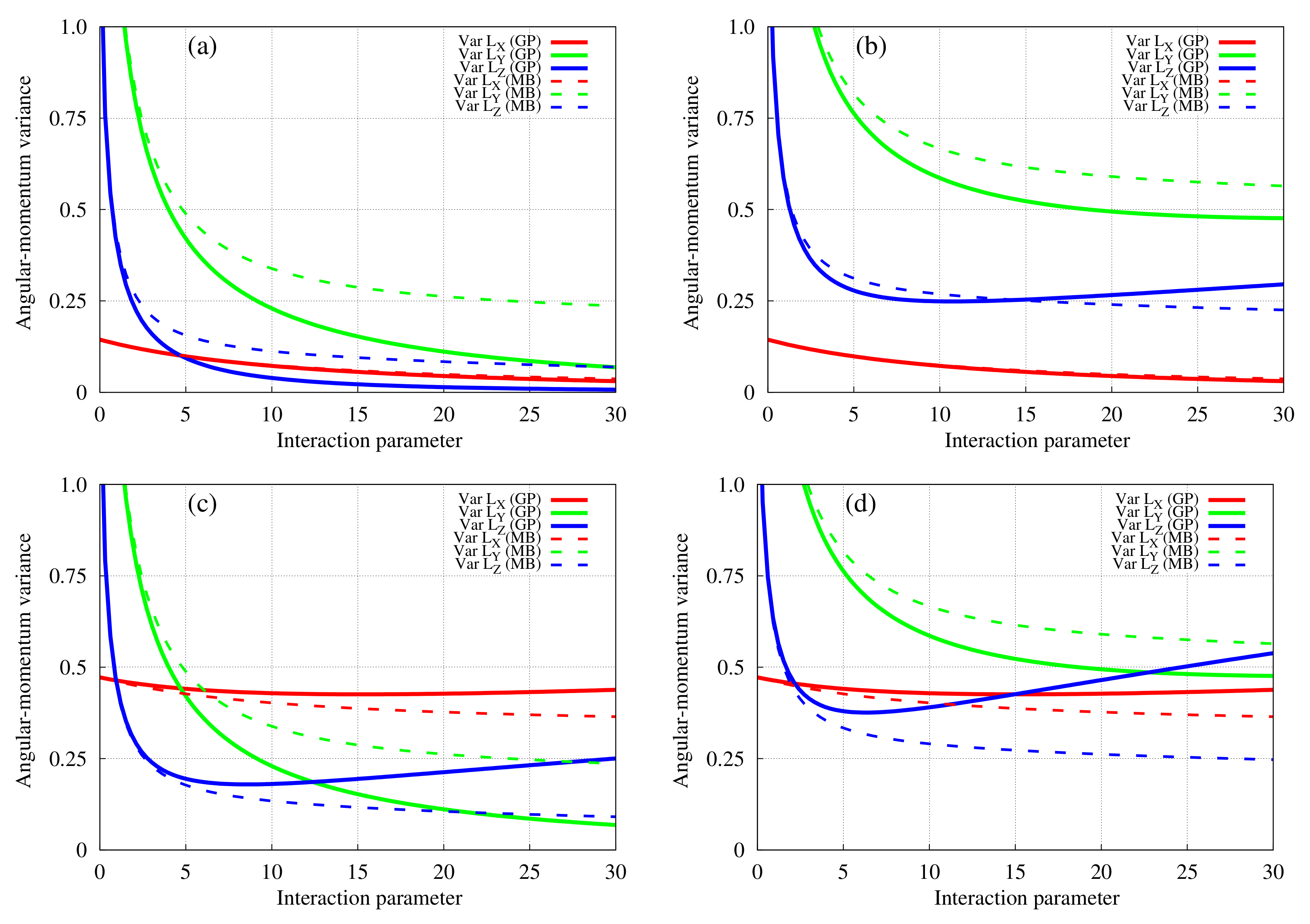
What happens as the interaction sets in? Figure 3a depicts the many-body and mean-field angular-momentum variances as a function of the interaction parameter $\Lambda$. We examine positive values of $\Lambda$ which correspond to the attractive sector of the harmonic-interaction model, see, e.g., [21,25,29]. Let us analyze the observations. With increasing interaction parameter the density narrows, along the x, y, and z directions. This is clear because the interaction between particles is attractive, and is manifested by the monotonously decreasing values of the position variances per particle (8). Furthermore, the density becomes less anisotropic, because the ratios of the dressed frequencies $\frac{\sqrt{{\omega }_z^2+2\Lambda }}{\sqrt{{\omega }_x^2+2\Lambda }}$, $\frac{\sqrt{{\omega }_y^2+2\Lambda }}{\sqrt{{\omega }_x^2+2\Lambda }}$, and $\frac{\sqrt{{\omega }_z^2+2\Lambda }}{\sqrt{{\omega }_y^2+2\Lambda }}$ monotonously decrease with increasing $\Lambda$. Consequently, the angular-momentum variances per particle decrease with the interaction parameter as well, see Figure 3a. The mean-field angular-momentum variances (9) are monotonously decreasing because of the just-described decreasing ratios of the dressed frequencies. The many-body angular-momentum variances are decreasing, at least for the values of interaction parameters studied here, because the positive-value correlations terms (10) grow slower than the mean-field angular-momentum variances decrease with $\Lambda$.

All in all, the anisotropy of the angular-momentum variance can now be determined. We find the anisotropy ${\mathrm{Var}|}_{\mathrm{MB}}({\widehat{L}}_Y)>{\mathrm{Var}|}_{\mathrm{MB}}({\widehat{L}}_Z)>{\mathrm{Var}|}_{\mathrm{MB}}({\widehat{L}}_X)$ to hold for all interaction parameters at the many-body level of theory. At the mean-field level of theory we find the same anisotropy, namely, ${\mathrm{Var}|}_{\mathrm{GP}}({\widehat{L}}_Y)>{\mathrm{Var}|}_{\mathrm{GP}}({\widehat{L}}_Z)>{\mathrm{Var}|}_{\mathrm{GP}}({\widehat{L}}_X)$, to hold for small interaction parameters. However, then, at just about $\Lambda =5.0$ the mean-field anisotropy changes to ${\mathrm{Var}|}_{\mathrm{GP}}({\widehat{L}}_Y)>{\mathrm{Var}|}_{\mathrm{GP}}({\widehat{L}}_X)>{\mathrm{Var}|}_{\mathrm{GP}}({\widehat{L}}_Z)$, and this anisotropy continues for larger interaction parameters. Hence, we have found that the anisotropy of the angular-momentum operator in the ground state of the three-dimensional anisotropic harmonic-interaction model at the infinite-particle-number limit changes as a function of the interaction parameter from the anisotropy class $\left\{1\right\}$ to $\{1,2\}$, see Figure 3a. In terms of the correlations term (1), the anisotropy of the variance is governed then by many-body effects.

Still, can the above-found picture of angular-momentum variance anisotropy be made richer? The answer is positive and requires one to dive deeper into the properties of angular-momentum variances under translations. To this end, we employ and extend prior work in two spatial dimensions [21]. Suppose now that the harmonic trap is located not in the origin but translated to a general point ${\mathbf{r}}_0=(x_0,y_0,z_0)$. The expectation values per particle of the momentum and angular-momentum operators are still zero, whereas the expectation value of the position operator is, of course, ${\mathbf{r}}_0$. Whereas the position and momentum variances are invariant to translations, the angular-momentum variances are not, which open up another degree of freedom to investigate the anisotropy class of the angular-momentum variances in three spatial dimensions. Mathematically, the transformation properties of the angular-momentum operator and its square combine in a non-trivial form those of the position and momentum operators. Physically, in a similar manner that angular momentum is defined with respect to a reference point, and it is different with respect to another reference point, so does the variance of the angular-momentum operator which changes with respect to distinct reference points.

Using the transformation properties of the angular-momentum operator $({\widehat{L}}_X,{\widehat{L}}_Y,{\widehat{L}}_Z)$ under translations, see Appendix A and [21], the final expressions for the translated angular-momentum variances per particle read explicitly

$$\begin{array}{c}{\mathrm{Var}|}_{\mathrm{MB}}({\widehat{L}}_X;{\mathbf{r}}_0)=\frac{1}{4}\frac{{\left(\sqrt{{\omega }_y^2+2\Lambda }-\sqrt{{\omega }_z^2+2\Lambda }\right)}^2}{\sqrt{{\omega }_y^2+2\Lambda }\sqrt{{\omega }_z^2+2\Lambda }}\left[1+\left(\sqrt{1+\frac{2\Lambda }{{\omega }_y^2}}-1\right)\left(\sqrt{1+\frac{2\Lambda }{{\omega }_z^2}}-1\right)\right]+\hfill \\ +y_0^2\frac{{\omega }_z}{2}+z_0^2\frac{{\omega }_y}{2},\hfill \\ {\mathrm{Var}|}_{\mathrm{MB}}({\widehat{L}}_Y;{\mathbf{r}}_0)=\frac{1}{4}\frac{{\left(\sqrt{{\omega }_z^2+2\Lambda }-\sqrt{{\omega }_x^2+2\Lambda }\right)}^2}{\sqrt{{\omega }_z^2+2\Lambda }\sqrt{{\omega }_x^2+2\Lambda }}\left[1+\left(\sqrt{1+\frac{2\Lambda }{{\omega }_z^2}}-1\right)\left(\sqrt{1+\frac{2\Lambda }{{\omega }_x^2}}-1\right)\right]+\hfill \\ +z_0^2\frac{{\omega }_x}{2}+x_0^2\frac{{\omega }_z}{2},\hfill \\ {\mathrm{Var}|}_{\mathrm{MB}}({\widehat{L}}_Z;{\mathbf{r}}_0)=\frac{1}{4}\frac{{\left(\sqrt{{\omega }_x^2+2\Lambda }-\sqrt{{\omega }_y^2+2\Lambda }\right)}^2}{\sqrt{{\omega }_x^2+2\Lambda }\sqrt{{\omega }_y^2+2\Lambda }}\left[1+\left(\sqrt{1+\frac{2\Lambda }{{\omega }_x^2}}-1\right)\left(\sqrt{1+\frac{2\Lambda }{{\omega }_y^2}}-1\right)\right]+\hfill \\ +x_0^2\frac{{\omega }_y}{2}+y_0^2\frac{{\omega }_x}{2}\hfill \end{array}$$

(11)

at the many-body level of theory and

$$\begin{array}{c}{\mathrm{Var}|}_{\mathrm{GP}}({\widehat{L}}_X;{\mathbf{r}}_0)=\frac{1}{4}\frac{{\left(\sqrt{{\omega }_y^2+2\Lambda }-\sqrt{{\omega }_z^2+2\Lambda }\right)}^2}{\sqrt{{\omega }_y^2+2\Lambda }\sqrt{{\omega }_z^2+2\Lambda }}+y_0^2\frac{\sqrt{{\omega }_z^2+2\Lambda }}{2}+z_0^2\frac{\sqrt{{\omega }_y^2+2\Lambda }}{2},\hfill \\ {\mathrm{Var}|}_{\mathrm{GP}}({\widehat{L}}_Y;{\mathbf{r}}_0)=\frac{1}{4}\frac{{\left(\sqrt{{\omega }_z^2+2\Lambda }-\sqrt{{\omega }_x^2+2\Lambda }\right)}^2}{\sqrt{{\omega }_z^2+2\Lambda }\sqrt{{\omega }_x^2+2\Lambda }}+z_0^2\frac{\sqrt{{\omega }_x^2+2\Lambda }}{2}+x_0^2\frac{\sqrt{{\omega }_z^2+2\Lambda }}{2},\hfill \\ {\mathrm{Var}|}_{\mathrm{GP}}({\widehat{L}}_Z;{\mathbf{r}}_0)=\frac{1}{4}\frac{{\left(\sqrt{{\omega }_x^2+2\Lambda }-\sqrt{{\omega }_y^2+2\Lambda }\right)}^2}{\sqrt{{\omega }_x^2+2\Lambda }\sqrt{{\omega }_y^2+2\Lambda }}+x_0^2\frac{\sqrt{{\omega }_y^2+2\Lambda }}{2}+y_0^2\frac{\sqrt{{\omega }_x^2+2\Lambda }}{2}\hfill \end{array}$$

(12)

at the mean-field level of theory. Let us examine expressions (11) and (12) more closely. The terms added to the translated angular-momentum variances at the many-body level depend on the corresponding components of the translation vector but not on the interaction parameter, whereas the added terms at the mean-field level of theory depend on and increase with $\Lambda$, see Appendix A for more details. The combined effects can be seen in Figure 3, compare panels Figure 3b–d with panel Figure 3a.

For the translation by ${\mathbf{r}}_0=(0.25,0,0)$, the angular-momentum variances ${\mathrm{Var}|}_{\mathrm{MB}}({\widehat{L}}_X;{\mathbf{r}}_0)$ and ${\mathrm{Var}|}_{\mathrm{GP}}({\widehat{L}}_X;{\mathbf{r}}_0)$ are invariant quantities, ${\mathrm{Var}|}_{\mathrm{MB}}({\widehat{L}}_Y;{\mathbf{r}}_0)$ and ${\mathrm{Var}|}_{\mathrm{MB}}({\widehat{L}}_Z;{\mathbf{r}}_0)$ are shifted by interaction-independent values, and ${\mathrm{Var}|}_{\mathrm{GP}}({\widehat{L}}_Y;{\mathbf{r}}_0)$ and ${\mathrm{Var}|}_{\mathrm{GP}}({\widehat{L}}_Z;{\mathbf{r}}_0)$ increase by interaction-dependent values, see (11) and (12), and compare Figure 3a,b. The combined effect is that now both ${\mathrm{Var}|}_{\mathrm{MB}}({\widehat{L}}_Y;{\mathbf{r}}_0)>{\mathrm{Var}|}_{\mathrm{MB}}({\widehat{L}}_Z;{\mathbf{r}}_0)>{\mathrm{Var}|}_{\mathrm{MB}}({\widehat{L}}_X;{\mathbf{r}}_0)$ and ${\mathrm{Var}|}_{\mathrm{GP}}({\widehat{L}}_Y;{\mathbf{r}}_0)>{\mathrm{Var}|}_{\mathrm{GP}}({\widehat{L}}_Z;{\mathbf{r}}_0)>{\mathrm{Var}|}_{\mathrm{GP}}({\widehat{L}}_X;{\mathbf{r}}_0)$ hold for all interaction parameters $\Lambda$ in the range studied. Consequently, the anisotropy class of the angular-momentum variance per particle for ${\mathbf{r}}_0=(0.25,0,0)$ is $\left\{1\right\}$ only.

Next, for ${\mathbf{r}}_0=(0,0.25,0)$, the angular-momentum variances ${\mathrm{Var}|}_{\mathrm{MB}}({\widehat{L}}_Y;{\mathbf{r}}_0)$ and ${\mathrm{Var}|}_{\mathrm{GP}}({\widehat{L}}_Y;{\mathbf{r}}_0)$ are invariant quantities, ${\mathrm{Var}|}_{\mathrm{MB}}({\widehat{L}}_X;{\mathbf{r}}_0)$ and ${\mathrm{Var}|}_{\mathrm{MB}}({\widehat{L}}_Z;{\mathbf{r}}_0)$ are shifted by interaction-independent values, and ${\mathrm{Var}|}_{\mathrm{GP}}({\widehat{L}}_X;{\mathbf{r}}_0)$ and ${\mathrm{Var}|}_{\mathrm{GP}}({\widehat{L}}_Z;{\mathbf{r}}_0)$ grow by interaction-dependent values, contrast Figure 3a,c. The combined effect is, of course, different than with ${\mathbf{r}}_0=(0.25,0,0)$, and we discuss its main features, focusing on the regime of interaction parameters larger than about $\Lambda =6$, for which the two many-body curves ${\mathrm{Var}|}_{\mathrm{MB}}({\widehat{L}}_X;{\mathbf{r}}_0)$ and ${\mathrm{Var}|}_{\mathrm{MB}}({\widehat{L}}_Y;{\mathbf{r}}_0)$ cross, see Figure 3c. The many-body angular-momentum variances satisfy ${\mathrm{Var}|}_{\mathrm{MB}}({\widehat{L}}_X;{\mathbf{r}}_0)>{\mathrm{Var}|}_{\mathrm{MB}}({\widehat{L}}_Y;{\mathbf{r}}_0)>{\mathrm{Var}|}_{\mathrm{MB}}({\widehat{L}}_Z;{\mathbf{r}}_0)$ for all studied interaction parameters. So, the effect of this translation is to alter the order of the many-body variances, i.e., to change the many-body anisotropy. Now, at the mean-field level, we find ${\mathrm{Var}|}_{\mathrm{GP}}({\widehat{L}}_X;{\mathbf{r}}_0)>{\mathrm{Var}|}_{\mathrm{GP}}({\widehat{L}}_Y;{\mathbf{r}}_0)>{\mathrm{Var}|}_{\mathrm{GP}}({\widehat{L}}_Z;{\mathbf{r}}_0)$ up to about $\Lambda =12$ and ${\mathrm{Var}|}_{\mathrm{GP}}({\widehat{L}}_X;{\mathbf{r}}_0)>{\mathrm{Var}|}_{\mathrm{GP}}({\widehat{L}}_Z;{\mathbf{r}}_0)>{\mathrm{Var}|}_{\mathrm{GP}}({\widehat{L}}_Y;{\mathbf{r}}_0)$ for the interaction parameters larger than about $\Lambda =12$. All in all, for the translation by ${\mathbf{r}}_0=(0.25,0,0)$ the above-described relations correspond, respectively, to the anisotropy classes $\left\{1\right\}$ and $\{1,2\}$ of the angular-momentum variances per particle.

Finally, for the translation by ${\mathbf{r}}_0=(0.25,0.25,0)$ non of the angular-momentum variances is invariant, see (11) and (12). The many-body angular-momentum variances ${\mathrm{Var}|}_{\mathrm{MB}}({\widehat{L}}_X;{\mathbf{r}}_0)$, ${\mathrm{Var}|}_{\mathrm{MB}}({\widehat{L}}_Y;{\mathbf{r}}_0)$, and ${\mathrm{Var}|}_{\mathrm{MB}}({\widehat{L}}_Z;{\mathbf{r}}_0)$ are shifted by interaction-independent values and the mean-field angular-momentum quantities ${\mathrm{Var}|}_{\mathrm{GP}}({\widehat{L}}_X;{\mathbf{r}}_0)$, ${\mathrm{Var}|}_{\mathrm{GP}}({\widehat{L}}_Y;{\mathbf{r}}_0)$, and ${\mathrm{Var}|}_{\mathrm{GP}}({\widehat{L}}_Z;{\mathbf{r}}_0)$ increase by interaction-dependent values, see Figure 3d. We examine the overall effect, concentrating on the regime of interaction parameters larger than about $\Lambda =2.5$, where the two many-body curves ${\mathrm{Var}|}_{\mathrm{MB}}({\widehat{L}}_X;{\mathbf{r}}_0)$ and ${\mathrm{Var}|}_{\mathrm{MB}}({\widehat{L}}_Z;{\mathbf{r}}_0)$ cross, see Figure 3d. The many-body angular-momentum variances satisfy ${\mathrm{Var}|}_{\mathrm{MB}}({\widehat{L}}_Y;{\mathbf{r}}_0)>{\mathrm{Var}|}_{\mathrm{MB}}({\widehat{L}}_X;{\mathbf{r}}_0)>{\mathrm{Var}|}_{\mathrm{MB}}({\widehat{L}}_Z;{\mathbf{r}}_0)$ for all interaction parameters in the range studied. Once again, the effect of the translation is to change the order of the many-body variances, thereby altering the many-body anisotropy, compare panels Figure 3a,c,d. At the mean-field level one finds ${\mathrm{Var}|}_{\mathrm{GP}}({\widehat{L}}_Y;{\mathbf{r}}_0)>{\mathrm{Var}|}_{\mathrm{GP}}({\widehat{L}}_X;{\mathbf{r}}_0)>{\mathrm{Var}|}_{\mathrm{GP}}({\widehat{L}}_Z;{\mathbf{r}}_0)$ up to about $\Lambda =15$, then ${\mathrm{Var}|}_{\mathrm{GP}}({\widehat{L}}_Y;{\mathbf{r}}_0)>{\mathrm{Var}|}_{\mathrm{GP}}({\widehat{L}}_Z;{\mathbf{r}}_0)>{\mathrm{Var}|}_{\mathrm{GP}}({\widehat{L}}_X;{\mathbf{r}}_0)$ till about $\Lambda =22.5$, and ${\mathrm{Var}|}_{\mathrm{GP}}({\widehat{L}}_Z;{\mathbf{r}}_0)>{\mathrm{Var}|}_{\mathrm{GP}}({\widehat{L}}_Y;{\mathbf{r}}_0)>{\mathrm{Var}|}_{\mathrm{GP}}({\widehat{L}}_X;{\mathbf{r}}_0)$ for all the interaction parameters larger than about $\Lambda =22.5$ studied, see Figure 3d. Therefore, for ${\mathbf{r}}_0=(0.25,0.25,0)$ the above-discussed findings imply that all anisotropy classes can be attained by the angular-momentum variances per particle in the three-dimensional harmonic-interaction model at the infinite-particle-number limit. These are, respectively, $\left\{1\right\}$, $\{1,2\}$, and $\{1,2,3\}$. In other words, we have shown that the correlations term (1) can dominate the angular-momentum properties of a trapped Bose–Einstein condensate at the limit of an infinite number of particles, which rounds off the present work.

4. Summary

The present work deals with a connection between anisotropy of and correlations in a three-dimensional trapped Bose–Einstein condensate. The merit of treating the limit of an infinite number of bosons is appealing, since the system is known to be 100% condensed in this limit, and some of its properties, notably the density per particle, are identical at the many-body and mean-field levels of theory.

We have analyzed the variances per particle of the three Cartesian components of the position ($\widehat{X},\widehat{Y},\widehat{Z}$), momentum (${\widehat{P}}_X,{\widehat{P}}_Y,{\widehat{P}}_Z$), and angular-momentum (${\widehat{L}}_X,{\widehat{L}}_Y,{\widehat{L}}_Z$) operators at the many-body and mean-field levels of theory. In general, for small interaction parameters the differences between the many-body and mean-field quantities are quantitative whereas for larger interaction parameters qualitative differences emerge. We define the anisotropy class of the variance according to the different orderings from large to small, or permutations, of the three respective many-body and mean-field quantities. The anisotropy class $\left\{1\right\}$ implies the same ordering, the class $\{1,2\}$ implies that two of the components are permuted, and the anisotropy class $\{1,2,3\}$ means that the three components are permuted.

Two relatively transparent applications are presented, the first is the breathing of an anisotropic three-dimensional trapped Bose–Einstein condensate, and the second is the ground state of the anisotropic three-dimensional harmonic-interaction model. The former exhibits different anisotropy classes of the position and momentum variances per particle, because at the many-body level the variances are constant, while at the mean-field level the variance of each component oscillates with a different amplitude and frequency, and consequently different anisotropy classes occur in time. The latter application shows different anisotropy classes of the angular-momentum variance per particle, owing to the intricate transformation properties of the angular-momentum variance when the wave-packet is translated from the origin. The challenge, which obviously goes beyond the scope of the present work, would be the experimental observation of such anisotropies and correlations. To access many-particle variances one would need to measure explicitly the positions, momenta, or angular-momenta of, in principle, all particles in the Bose–Einstein condensate, rather than just the total density from which the expectation values of these observables can be deduced.

To sum up, the anisotropy or morphology of a three-dimensional trapped Bose–Einstein condensate can look quite different when examined through the ‘glasses’ of many-body and mean-field theories, even for 100% condensed bosons at the limit of an infinite number of particles. It would be interesting to conduct the investigation presented here and analyze the results in more complicated numerical many-particle scenarios. Last but not least, it is possible to envision classifying the morphology of a Bose–Einstein condensate beyond that emanating from the variances of the position, momentum, and angular-momentum operators. Furthermore, in four spatial dimensions one could expect an additional richness of the variance [38].

References

- Castin, Y.; Dum, R. Low-temperature Bose–Einstein condensates in time-dependent traps: Beyond the U(1) symmetry breaking approach. Phys. Rev. A 1998, 57, 3008. [Google Scholar] [CrossRef] [Green Version]
- Lieb, E.H.; Seiringer, R.; Yngvason, J. Bosons in a trap: A rigorous derivation of the Gross–Pitaevskii energy functional. Phys. Rev. A 2000, 61, 043602. [Google Scholar] [CrossRef] [Green Version]
- Lieb, E.H.; Seiringer, R. Proof of Bose–Einstein Condensation for Dilute Trapped Gases. Phys. Rev. Lett. 2002, 88, 170409. [Google Scholar] [CrossRef] [PubMed] [Green Version]
- Erdos, L.; Schlein, B.; Yau, H.-T. Rigorous Derivation of the Gross–Pitaevskii Equation. Phys. Rev. Lett. 2007, 98, 040404. [Google Scholar] [CrossRef] [Green Version]
- Erdos, L.; Schlein, B.; Yau, H.-T. Derivation of the cubic non-linear Schrödinger equation from quantum dynamics of many-body systems. Invent. Math. 2007, 167, 515. [Google Scholar] [CrossRef] [Green Version]
- Klaiman, S.; Alon, O.E. Variance as a sensitive probe of correlations. Phys. Rev. A 2015, 91, 063613. [Google Scholar] [CrossRef] [Green Version]
- Klaiman, S.; Streltsov, A.I.; Alon, O.E. Uncertainty product of an out-of-equilibrium many-particle system. Phys. Rev. A 2016, 93, 023605. [Google Scholar] [CrossRef] [Green Version]
- Klaiman, S.; Cederbaum, L.S. Overlap of exact and Gross–Pitaevskii wave functions in Bose–Einstein condensates of dilute gases. Phys. Rev. A 2016, 94, 063648. [Google Scholar] [CrossRef] [Green Version]
- Anapolitanos, I.; Hott, M.; Hundertmark, D. Derivation of the Hartree equation for compound Bose gases in the mean field limit. Rev. Math. Phys. 2017, 29, 1750022. [Google Scholar] [CrossRef] [Green Version]
- Michelangeli, A.; Olgiati, A. Mean-field quantum dynamics for a mixture of Bose–Einstein condensates. Anal. Math. Phys. 2017, 7, 377. [Google Scholar] [CrossRef]
- Alon, O.E. Solvable model of a generic trapped mixture of interacting bosons: Reduced density matrices and proof of Bose–Einstein condensation. J. Phys. A 2017, 50, 295002. [Google Scholar] [CrossRef] [Green Version]
- Cederbaum, L.S. Exact many-body wave function and properties of trapped bosons in the infinite-particle limit. Phys. Rev. A 2017, 96, 013615. [Google Scholar] [CrossRef]
- Coleman, A.J.; Yukalov, V.I. Reduced Density Matrices: Coulson’s Challenge; Lectures Notes in Chemistry; Springer: Berlin, Germany, 2000; Volume 72. [Google Scholar]
- Mazziotti, D.A. (Ed.) Reduced-Density-Matrix Mechanics: With Application to Many-Electron Atoms and Molecules; Advances in Chemical Physics; Wiley: New York, NY, USA, 2007; Volume 134. [Google Scholar]
- Lode, A.U.J.; Lévêque, C.; Madsen, L.B.; Streltsov, A.I.; Alon, O.E. Colloquium: Multiconfigurational time-dependent Hartree approaches for indistinguishable particles. Rev. Mod. Phys. 2020, 92, 011001. [Google Scholar] [CrossRef] [Green Version]
- Bolsinger, V.J.; Krönke, S.; Schmelcher, P. Ultracold bosonic scattering dynamics off a repulsive barrier: Coherence loss at the dimensional crossover. Phys. Rev. A 2017, 96, 013618. [Google Scholar] [CrossRef] [Green Version]
- Alon, O.E. Condensates in annuli: Dimensionality of the variance. Mol. Phys. 2019, 117, 2108. [Google Scholar] [CrossRef] [Green Version]
- Klaiman, S.; Beinke, R.; Cederbaum, L.S.; Streltsov, A.I.; Alon, O.E. Variance of an anisotropic Bose–Einstein condensate. Chem. Phys. 2018, 509, 45. [Google Scholar] [CrossRef] [Green Version]
- Sakmann, K.; Schmiedmayer, J. Conserving symmetries in Bose–Einstein condensate dynamics requires many-body theory. arXiv 2018, arXiv:1802.03746v2. [Google Scholar]
- Streltsov, A.I.; Streltsova, O.I. MCTDHB-LAB, Version 1.5. 2015. Available online: http://www.mctdhb-lab.com (accessed on 10 May 2021).
- Alon, O.E. Analysis of a Trapped Bose–Einstein Condensate in Terms of Position, Momentum, and Angular-Momentum Variance. Symmetry 2019, 11, 1344. [Google Scholar] [CrossRef] [Green Version]
- Robinson, P.D. Coupled oscillator natural orbitals. J. Chem. Phys. 1977, 66, 3307. [Google Scholar] [CrossRef]
- Hall, R.L. Some exact solutions to the translation-invariant N-body problem. J. Phys. A 1978, 11, 1227. [Google Scholar] [CrossRef]
- Hall, R.L. Exact solutions of Schrödinger’s equation for translation-invariant harmonic matter. J. Phys. A 1978, 11, 1235. [Google Scholar] [CrossRef]
- Cohen, L.; Lee, C. Exact reduced density matrices for a model problem. J. Math. Phys. 1985, 26, 3105. [Google Scholar] [CrossRef]
- Osadchii, M.S.; Muraktanov, V.V. The System of Harmonically Interacting Particles: An Exact Solution of the Quantum-Mechanical Problem. Int. J. Quant. Chem. 1991, 39, 173. [Google Scholar] [CrossRef]
- Załuska-Kotur, M.A.; Gajda, M.; Orłowski, A.; Mostowski, J. Soluble model of many interacting quantum particles in a trap. Phys. Rev. A 2000, 61, 033613. [Google Scholar] [CrossRef] [Green Version]
- Yan, J. Harmonic Interaction Model and Its Applications in Bose–Einstein Condensation. J. Stat. Phys. 2003, 113, 623. [Google Scholar] [CrossRef]
- Gajda, M. Criterion for Bose–Einstein condensation in a harmonic trap in the case with attractive interactions. Phys. Rev. A 2006, 73, 023603. [Google Scholar] [CrossRef]
- Armstrong, J.R.; Zinner, N.T.; Fedorov, D.V.; Jensen, A.S. Analytic harmonic approach to the N-body problem. J. Phys. B 2011, 44, 055303. [Google Scholar] [CrossRef] [Green Version]
- Armstrong, J.R.; Zinner, N.T.; Fedorov, D.V.; Jensen, A.S. Virial expansion coefficients in the harmonic approximation. Phys. Rev. E 2012, 86, 021115. [Google Scholar] [CrossRef] [Green Version]
- Schilling, C. Natural orbitals and occupation numbers for harmonium: Fermions versus bosons. Phys. Rev. A 2013, 88, 042105. [Google Scholar] [CrossRef] [Green Version]
- Benavides-Riveros, C.L.; Toranzo, I.V.; Dehesa, J.S. Entanglement in N-harmonium: Bosons and fermions. J. Phys. B 2014, 47, 195503. [Google Scholar] [CrossRef]
- Bouvrie, P.A.; Majtey, A.P.; Tichy, M.C.; Dehesa, J.S.; Plastino, A.R. Entanglement and the Born-Oppenheimer approximation in an exactly solvable quantum many-body system. Eur. Phys. J. D 2014, 68, 346. [Google Scholar] [CrossRef]
- Armstrong, J.R.; Volosniev, A.G.; Fedorov, D.V.; Jensen, A.S.; Zinner, N.T. Analytic solutions of topologically disjoint systems. J. Phys. A 2015, 48, 085301. [Google Scholar] [CrossRef] [Green Version]
- Schilling, C.; Schilling, R. Number-parity effect for confined fermions in one dimension. Phys. Rev. A 2016, 93, 021601(R). [Google Scholar] [CrossRef] [Green Version]
- Alon, O.E. Variance of a Trapped Bose–Einstein Condensate. J. Phys. Conf. Ser. 2019, 1206, 012009. [Google Scholar] [CrossRef] [Green Version]
- Yukalov, V.I. Particle Fluctuations in Mesoscopic Bose Systems. Symmetry 2019, 11, 603. [Google Scholar] [CrossRef] [Green Version]
Figure 1.
Many-particle position (, , and ; in red, green, and blue) variance per particle as a function of time computed at the limit of an infinite number of particles within many-body (dashed lines) and mean-field (solid lines) levels of theory in an interaction-quench scenario. The harmonic trap is 10% anisotropic in panels (a,c,e,g) and 20% anisotropic in panels (b,d,f,h). The coupling constant g is indicated in each panel. Different anisotropy classes of the position variance emerge with time. See the text for more details. The quantities shown are dimensionless.
Figure 2.
Many-particle momentum (, , and ; in red, green, and blue) variance per particle as a function of time computed at the infinite-particle-number limit within many-body (dashed lines) and mean-field (solid lines) levels of theory in an interaction-quench scenario. The harmonic trap is 10% anisotropic in panels (a,c,e,g) and 20% anisotropic in panels (b,d,f,h). The coupling constant g is indicated in each panel. Different anisotropy classes of the momentum variance emerge with time. See the text for more details. The quantities shown are dimensionless.
Figure 3.
Many-particle angular-momentum (, , and ; in red, green, and blue) variance per particle as a function of the interaction parameter computed at the limit of an infinite number of particles within many-body (dashed lines) and mean-field (solid lines) levels of theory for the ground state of the three-dimensional anisotropic harmonic-interaction model. The frequencies of the trap are , , and . Results at several translations of the center of the trap are shown in the panels: (a) ; (b) ; (c) ; (d) . Different anisotropy classes of the angular-momentum variance emerge with the interaction parameter. See the text for more details. The quantities shown are dimensionless.
Publisher’s Note: MDPI stays neutral with regard to jurisdictional claims in published maps and institutional affiliations. |
© 2021 by the author. Licensee MDPI, Basel, Switzerland. This article is an open access article distributed under the terms and conditions of the Creative Commons Attribution (CC BY) license (https://creativecommons.org/licenses/by/4.0/).
Share and Cite
MDPI and ACS Style
Alon, O.E. Morphology of an Interacting Three-Dimensional Trapped Bose–Einstein Condensate from Many-Particle Variance Anisotropy. Symmetry 2021, 13, 1237. https://0-doi-org.brum.beds.ac.uk/10.3390/sym13071237
AMA Style
Alon OE. Morphology of an Interacting Three-Dimensional Trapped Bose–Einstein Condensate from Many-Particle Variance Anisotropy. Symmetry. 2021; 13(7):1237. https://0-doi-org.brum.beds.ac.uk/10.3390/sym13071237
Chicago/Turabian StyleAlon, Ofir E. 2021. "Morphology of an Interacting Three-Dimensional Trapped Bose–Einstein Condensate from Many-Particle Variance Anisotropy" Symmetry 13, no. 7: 1237. https://0-doi-org.brum.beds.ac.uk/10.3390/sym13071237
Note that from the first issue of 2016, this journal uses article numbers instead of page numbers. See further details here.