
Task Decomposition Based on Cloud Manufacturing Platform

School of Mechatronic Engineering, Changchun University of Technology, Changchun 130012, China
*
Author to whom correspondence should be addressed.
Symmetry 2021, 13(8), 1311; https://0-doi-org.brum.beds.ac.uk/10.3390/sym13081311
Submission received: 14 June 2021
/
Revised: 11 July 2021
/
Accepted: 19 July 2021
/
Published: 21 July 2021
(This article belongs to the Special Issue Asymmetric and Symmetric Study on Digital Twins and Cyber-Physical-Social Systems)
Abstract
:As a new service-oriented manufacturing paradigm, cloud manufacturing (CMfg) realizes the optimal allocation of resources in the product manufacturing process through the network. Task decomposition is a key problem of the CMfg system for resource scheduling. A high-quality task decomposition method can shorten product development time, reduce costs for resource service providers, and provide technical support for the application of CMfg. However, a cloud manufacturing system has to manage the allocation the correct amount of manufacturing resources, complex production processes, and highly dynamic production environments. At the same time, the tasks issued by service demanders are usually asymmetric and tightly coupled. We solve the complex task decomposition problem by using the traditional methods, that are hard to complete in CMfg. To overcome the shortcomings of CMfg, this paper proposed a task decomposition method based on the cloud platform. For achieving modular production, this approach creatively divides the product production process into four stages: design, manufacturing, transportation, and maintenance. Then a hybrid method, which combines with depth-first search algorithm, fast modular optimization algorithm, and artificial bee colony algorithm, is introduced. The method can obtain a multi-stage task optimization decomposition plan in CMfg. Simulation results demonstrate the proposed method can achieve complex task optimization decomposition in a CMfg environment.
1. Introduction
The use of features such as customization and specialization in order to meet market demands has put manufacturing industry in a prominent position. In a dynamic manufacturing environment, cooperation and sharing are mainstream ideas [1]. At the same time, high adaptability and agility are vital for an enterprise to maintain competitiveness. On one hand, cooperation and sharing between enterprises can shorten the product’s time-to-market. Similarly, the cost of research and development for the enterprise can be reduced. On the other hand, highly adaptability and agility allow enterprises to fulfill customer’s individual demands. The ability of manufacturing companies to manage unknown risks can be strengthened. Consequently, manufacturing enterprises must improve their production strategies and manufacturing mode to face this challenge.
For the past ten years, cloud manufacturing (CMfg) as a new manufacturing paradigm that integrates information technology (such as cloud computing [2], internet of things [3], service-oriented technologies [4], blockchain technologies [5,6], and so forth) and advanced manufacturing technology, has attracted broad attention in both industry and the academic community. Cloud manufacturing centralized the sharing of decentralized resources by establishing a public cloud service platform. Cloud platforms encapsulated manufacturing resources into manufacturing services, centralized management and operations, and provided on-demand manufacturing services according to customers’ demands [7]. The optimization of task scheduling in the cloud manufacturing system can effectively optimize the quality of service, and task decomposition plays a vital role in task scheduling. Task decomposition can reduce the complexity of scheduling and provide a theoretical foundation for large-scale collaborative manufacturing.
The task decomposition based on a cloud manufacturing platform uses the existing production factors and the requirements of the customers as the driving forces, and divides the manufacturing tasks on the cloud into several realistic production processes. To address the task division problem of the cloud platform it is necessary to establish a relevant mathematical model according to the actual situation. On the other hand, we also need to select a suitable algorithm, based on the characteristics of the mathematical model, to provide high-quality resources for the manufacturing tasks in the resource pool. The process of task decomposition is to divide cumbersome manufacturing processes into several brief process stages, according to a set of rules. Then, we divide the tasks into subtasks with an appropriate granularity, and form different sets of subtasks through these stages.
However, fewer considered features or more restrictive conditions make the task decomposition differ in actual situations, compared to those described in existing research. For example, product production process division and task relationship constraints have a greater impact on product quality. The existing works seldom take these characteristics into account as a critical influence factor. The proposed approaches mostly ignored interference, or considered fixed disturbances during task decomposition. These proposed approaches lack a capacity to manage unexpected disturbances, such as machine breakdown, logistic delay, order change, etc. Most of proposed task decomposition methods consider the single scheduling index and the tasks with symmetrical structure.
With the consideration of the above situations, a task decomposition method based on the cloud platform is designed. In the method, complex tasks are divided into multiple stages according to the attributes and characteristics of the production process, this makes production processes in all stages more convenient. At the same time, the novel hybrid method combines depth first search, fast modular, and artificial bee colony to optimize multi-stage production processes. The method can achieve the adaptive resource scheduling in CMfg system that has massive manufacturing resource and high-dimensional coupled manufacturing tasks. Meanwhile, logistics, transportation, maintenance, and other requirements in task decomposition are considered, this makes the decomposition approach of this paper more applicable. Simulation results demonstrate the effectiveness of the task decomposition method.
2. Literature Review
Task decomposition is vital for the optimal allocation of resources in CMfg scheduling, and, therefore, this has attracted broad attention in the manufacturing industry. At present, task decomposition theory and methods under traditional modes have been widely researched. Wang et al. investigated the correlation between the subtasks in the internal structure, and presented it by axiomatic matrix based on the information flow relationship of the subtasks [8]. Yu et al. proposed a task decomposition method based on the state variables of the dynamic Bayesian network model [9]. Zhou et al. proposed a hierarchical decomposition method that divides all elements in production, from individual to whole, from parts to components. The method properly solved the problem of unrealistic task decomposition in production and the scattered resource allocation [10]. Weiss et al. proposed a hierarchical decomposition methodology in smart manufacturing, the method decomposes manufacturing processes to user-defined levels [11]. Garashcheoko et al. studied the connection between features of part construction and task decomposition in additive manufacturing process, and evaluate the effectiveness of parts decomposition [12]. Dikici et al. decomposed complex tasks into a set of subtasks according to requirements, which can improve the comprehensibility of the process and reduce the difficulty of analysis [13].
Research about task decomposition in CMfg is in its formative stages. Liu et al. proposed a decomposition method based on the execution order of CMfg tasks, and the method uses a recursive decomposition algorithm to optimize task decomposition processes at different levels [14]. To solve complex parts machining problems in CMfg, Guo et al. presented a machining task decomposition strategy which uses features of the complex part as task granularity [15]. Zhang et al. proposed a two-stage decomposition algorithm based on global manufacturing business process network (GMPBN) in CMfg, which can decompose and refine the cumbersome manufacturing links [16]. A complex manufacturing task decomposition method, which considered three significant factors: resource, workflow, and activity under CMfg environment, was presented in [17].
In conclusion, even though task decomposition in a traditional manufacturing environment has been well studied, the proposed methods are generally inappropriate for service-oriented manufacturing paradigms, such as CMfg, as a lot of essential factors are not considered. Recently, some novel algorithms have been introduced in manufacturing systems, which have brought new perspectives for the research of cloud manufacturing task decomposition. However, they only focus on task granularity and ignore the connection between the attributes of the task itself and task decomposition. In the meantime, most of the research works rely on experiences that have high subjectivity, and they result in error or inaccurate results. The cloud platform will be required to decompose massive and complex production tasks, which is a huge challenge for the application of cloud manufacturing. Consequently, it is urgent to establish a method based in the cloud platform for addressing the task decomposition problem in CMfg.
3. Task Decomposition and Theoretical Model
According to the production cycle of the product, the paper divides the task into multiple stages, including design stage, manufacturing stage, transportation stage, and maintenance stage; the relationship between them is shown in Figure 1.
Based on intelligent planning methods, hierarchical task network (HTN) planning methods apply a tree diagram to gradually decompose a complex and asymmetric overall task into subtasks that can be directly executed [18]. The tasks planned by HTN can be presented by triples , S refers to the transition state of the tasks that indicate whether the task is completely decomposition. As the list of n tasks that need to be planned, represents the sequence of task planning. D is the domain of discourse, which is a set of operations and methods, representing the decomposition methods corresponding to different task stages. Based on the HTN planning method, the cloud platform can enable complex asymmetric manufacturing tasks to achieve the best decomposition plan at each stage of the production cycle. Each stage is related and can be executed independently. At the same time, one or more stages of task decomposition can be performed according to actual production requirements. Therefore, the paper focuses on decomposing the manufacturing project into tasks with appropriate granularity and easy processing.
3.1. Design Tasks Decomposition Model
The essence of product design is through matching the design to the requirements it needs to satisfy. In parallel design, people of different disciplines, levels, and expertise are gathered together to complete the design work. At the beginning of project, the design work should take into account the entire lifecycle of the designed product, and coordinate the design of the product through multi-type and multi-department cooperation. It can effectively condense the manufacturing cost of the enterprise, shorten the production cycle of the product, and increase the design efficiency of the product.
During the design process, there are complex relations among each task, such as direct information interaction, restraining, and interdependence. The design objective is to arrange all subtasks into an optimal sequence. There is a certain degree of communication between the subtasks. We split and combine subtasks with a high degree of contact, while reducing the communication between subtask groups to maintain a high degree of independence. Therefore, this paper introduces the concept of task association coupling degree in the process of design task decomposition. The following requirements are the content that the cloud platform needs to ensure:
- Subtasks need to satisfy the designer. The decomposed subtasks should satisfy the designer as much as possible. The feedback of the design system is used to verify the results of the task decomposition and realize the correction of the decomposition results;
- Minimum coupling value of subtask. In the design process, the closely related subtasks are combined together through task coupling and form a module. At the same time, reducing the information interaction between the modules makes each module relatively independent, so as to reduce the development time and improve the quality of the product;
- Subtasks retain special design requirements. For certain design tasks, customers’ demands on the design should be considered. Retain the user’s special requirements on product design, and ensure the integrity of the special structure or processing method during the product design process to prevent it from being disassembled;
- The granularity of subtasks should be moderate. Granularity is a general summary of the number of subtasks and the division of levels. When the granularity is small, that is not convenient for management of subtasks. When the granularity is large, that is inconvenient to decompose the subtasks. Therefore, it is necessary to continuously optimize the decomposition granularity through the task decomposition mechanism, and finally obtain a moderate subtask granularity.
We can define as satisfaction, j as design group, and as task. The represents the degree of satisfaction of the design team with the task. Satisfaction can set a fuzzy set of variables, the subset is very dissatisfied, dissatisfied, general, satisfied, and very satisfied. At the same time, the five situations are intuitively quantified with data: 0, 0.25, 0.5, 0.75, 1. Average satisfaction can be calculated by Equation (1).
We regard the design task as an overall task and decompose it into several subtasks according to the functional characteristics. When the subtask cannot be decomposed further, it is called the smallest subtask. If it can continue to be decomposed, the satisfaction test of the subtask can be performed by Formula (1). At this time, we have to introduce a concept about the threshold λ. The value range of λ is between 0 and 1, and the specific value depends on the situation. The specific decomposition steps are as follows:
- Consider the product design task as an overall task and decompose it into several subtasks according to functional categories, ;
- When the subtask cannot continue to be decomposed, the decomposition process is terminated. If task can continue to decompose, we can use Formula (1) to perform a satisfaction test on this subtask;
- If the satisfaction degree is lower than the threshold λ, the subtask continues to be decomposed until the satisfaction degree of the decomposed subtask is higher than the set threshold λ;
- Judge the overall rationality and complete the tree structure decomposition of the design task.
For the specific definition of satisfaction , we take account into three aspects: platform layer, service layer, and customer layer. Platform layers include structural satisfaction, material satisfaction, and feasibility satisfaction. Service layers include personnel quality, service prices, and design concepts. Customer layer include performance requirements and credibility. It should be noted that the average satisfaction degree needs to meet the specified standards of subtask and overall attribute requirements of the product.
According to the above decomposing methods, a tree structure with various levels is formed. We define T as a task, are decomposed subtasks, are subtasks decomposed by task , and the value of the subscript indicates the task hierarchy and subordinate relationship.
In order to reflect the relevance of the subtasks, we build a design structure matrix based on the task node data. The dimension of the design structure matrix represents the number of design tasks, the rows of the matrix represent the task output support required to complete the task, and the columns of the matrix represent the input support of the task required to complete the task. In the matrix of Equation (2), A represents the matrix itself. The matrix consists of n tasks. The tasks can be represented by , and the diagonal elements represent the design task. The information flow between various design tasks is generally represented by . When task Ti has information circulation to task Tj, = 1, and task T_i has no information circulation to task Tj, = 0.
We need to clarify the connection between different subtasks when design the structure matrix. This paper uses a method based on fuzzy set theory to solve this problem. In the design task decomposition of cloud manufacturing, a set of fuzzy variables is set according to the size of the interaction between design subtasks. This set is represented by the following five seed sets: weak, weaker, medium, stronger, and strong, and this can be quantified with data: 0, 0.25, 0.5, 0.75, 1. Represent the various elements by the value in the matrix, and transform the matrix A into the numeric matrix P in Equation (3). On the one hand, the matrix can clearly know the information flow in various design tasks, and it can indicate the degree of connection between tasks.
3.2. Manufacturing Tasks Decomposition Model
Now, the complexity of the product structure is getting higher. An accessory can be composed of thousands of parts, and there are some interdependencies between these parts. We decompose the manufacturing tasks according to the feature to receive the manufacturing process that meets the requirements.
The information that is no longer needed for interaction between manufacturing tasks since it comes from design tasks, and the task only decomposed into different manufacturing subtasks according to the characteristic of the design tasks. The manufacturing tasks submitted to the CMfg can be decomposed into different subtask directed graphs according to the task type, and the dependency relationship between the subtasks determines the manufacturing sequence. Therefore, the following five principles must be guaranteed when the manufacturing tasks are decomposed:
- Subtask matching principle. The decomposed subtasks are delivered to the workshop, and the resources in the resource pool must available for subtasks;
- Subtask relatively independent principle. The production requirements should be met in the process of designing products. The steps that are processed at one time should be gathered together. Prevent unnecessary damage to processed products during subsequent transportation, leading to increase in cost and scrap rate;
- Subtask management and control principle. The number of subtasks should be convenient to control and the workload was close. The complex tasks are equally divided into the subtask groups to ensure the maximum completion time between contents is similar. At the same time, the completion of the overall task is guaranteed to avoid affecting the overall progress due to the delay of subtasks;
- The maximum subtask cohesion principle. We introduce the aggregation coefficient between subtasks when the task decomposition scheme is available, and the largest sum of aggregation values between groups need to be selected;
- Special manufacturing principle. For special components that need to be processed, if it is continuous processing without interval or special treatment after the completion of the process, it is necessary to maintain the integrity of the processing process.
In the manufacturing task, the process steps are clear. They are all completed step by step from process to part, from part to part, and from part to product. The hierarchy is clearly divided and the connection is relatively close. Work breakdown structure (WBS) is a task decomposition method that decomposes a project into a hierarchical structure based on internal relationships. It refers to likewise product structures in the cloud platform product library, and relies on WBS to make manufacturing tasks easier to decompose. Dividing manufacturing tasks into the process level requires huge transportation costs. Therefore, the smallest production and manufacturing task unit are generally set at the part level.
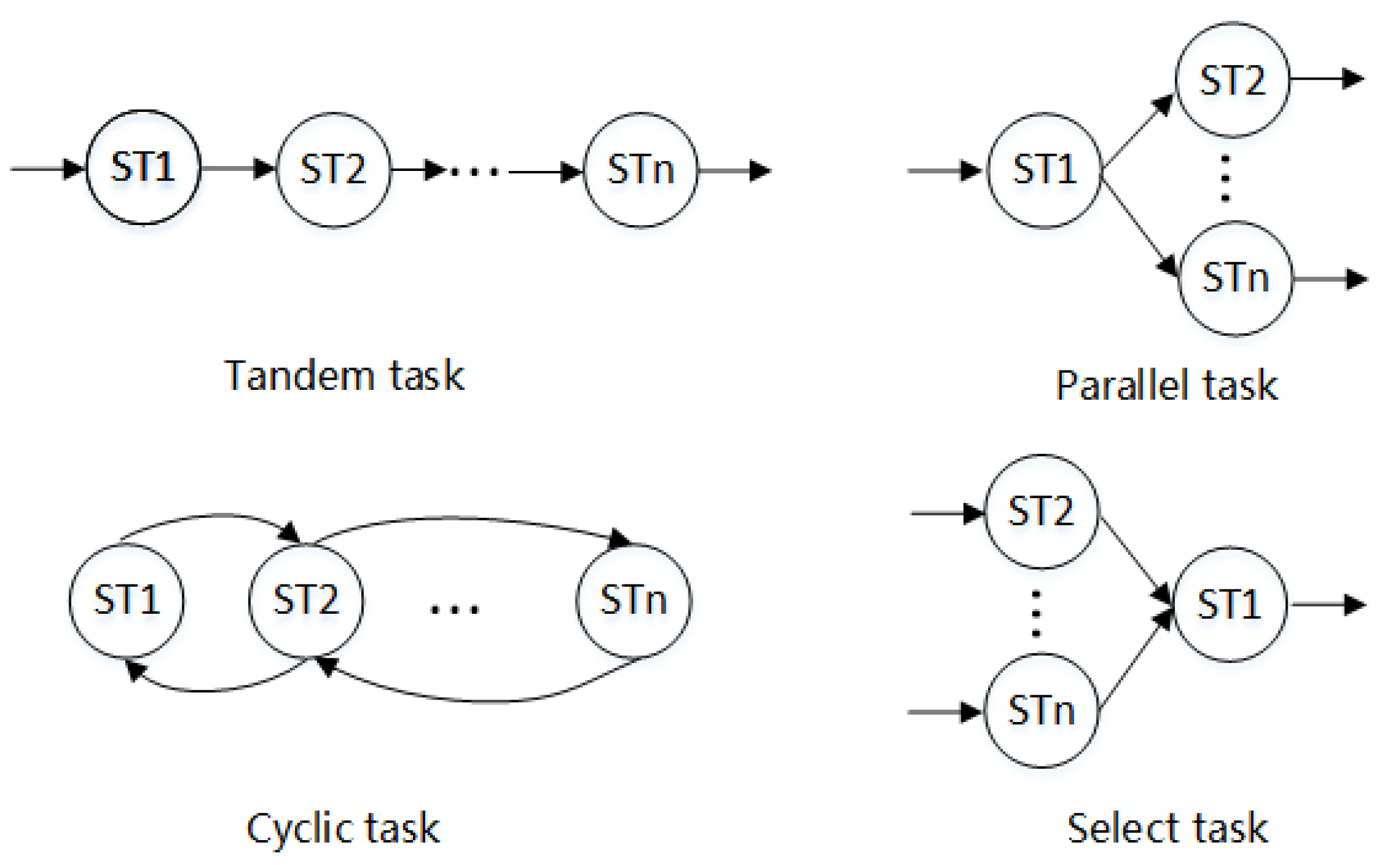
The minimum tasks of cloud manufacturing have a strong mutual constraint relationship, and the order of these tasks is relatively fixed. The tasks constraint structures can be divided into four categories (Figure 2): serial, parallel, loop, selection. The serial constraint structure means that subtasks of the production task have a clear sequence. Parallel constraint means that there is no clear sequence of subtasks of the production task. Cycle constraints mean that these subtasks can be completed in multiple cycles. Selection constraint means that the manufacture method can be determined according to the production situation during the production process. Based on the structure of task constraints, calculate the relationship values between tasks by Equations (4)–(6) to obtain the cohesion coefficient between manufacturing tasks.
In the task correlation coefficient , where |t| represents the number of meta-tasks, and are output meta-tasks, and di are input meta-tasks. The numerator represents the number of exchanges among subtasks when ≠. The detail is shown in Equation (4).
In Equation (5), the task reuse coefficient refers to the ratio of the meta-tasks that are repeatedly used in the subtasks to all the meta-tasks, and the larger ratio represents frequent communication between tasks. The task cohesion coefficient is a comprehensive measure of task cohesion. It is the product of the task correlation coefficient and the task reuse coefficient , which can be calculated by Equation (6):
The task cohesion coefficient represents the correlation level of each subtask in the production task. Its correlation level can reflect the workload of the subtasks, that is, the granularity. The granularity of subtasks can be explained by two indicators: task granularity coefficient and number of tasks. The larger the task granularity coefficient, the fewer the number of subtasks, the task decomposition is not in place, and the manufacturing work is complicated. The smaller the task granularity factor, the more tasks there are, which means more subtasks. In order to avoid the high degree aggregation of subtasks in the production process, we decompose the subtasks into the meta-task layer and introduce coupling coefficients to ensure the rationality of the aggregation results. We use Ai represents the task coupling coefficient, ci represents the cohesion coefficient. Then the expression of granularity can be measured by the coupling coefficient, which can be calculated by Equation (7):
The overall task granularity of CMfg can be expressed by the average granularity measurement of each subtask, which can be calculated by Equation (8):
When is larger, the configuration of task granularity is unreasonable, and the degree of cohesion of various subtasks decomposed by cloud tasks is lower. We build a matrix based on the above calculation results to structure decomposition model of the manufacturing task.
3.3. Transportation Task Decomposition Model
The transportation task is generated based on the resource interaction between the manufacturing subtasks that are decomposed into a grid. The transportation services are restricted by region and transportation volume, transportation tasks also need to be decomposed into several subtasks according to the attributes of manufacturing tasks [19]. We can, respectively, match the appropriate transportation resources, so as to achieve the maximize transportation efficiency. The corresponding mathematical model is shown as below:
- Transport time objective function (T)
According to the requirements of the transportation task, search and match the transportation resources in the candidate resource set. Transportation resource optimization time is defined by Equation (9):
is the deadline delivery date, and the constraints of transportation time (T) is shown by Equation (10):
- 2.
- Transportation cost objective function (C)
According to the requirements of the manufacturing task, the manufacturing resources in the candidate resource set are searched and matched. Transportation cost function of the optimized matching of the manufacturing resources is defined by Equation (11):
where represents the maximum cost specified by the customer, and the constraints of transportation cost (C) is shown by Equation (12):
- 3.
- Transportation quality objective function (Q)
According to the requirements of the manufacturing task, the manufacturing resources in the candidate resource set are searched and matched. The processing quality function for optimal matching of manufacturing resources is shown by Equation (13):
where represents the minimum service quality specified by the customer, and the constraints of transportation quality (Q) is shown by Equation (14):
- 4.
- Transportation capacity objective function()
According to the requirements of transportation tasks, search and match the transportation resources in the candidate resource set. represents the maximum load capacity at each stage of the transportation service. The transportation resource capacity is shown by Equation (15):
3.4. Maintenance Task Decomposition Model
Maintenance tasks run through the entire product processing stage. There are differences in maintenance tasks in terms of maintenance type, maintenance technology level, and maintenance workload. Therefore, we can decompose maintenance tasks according to different types and workloads. Types can be divided into three types: advance prevention, emergency maintenance, and targeted maintenance. The workload is also divided into three types: large, medium, and small. Refer to the idea of fuzzy sets for fuzzy classification, and complete the selection under the condition of meeting the technical requirements and workload.
The sort of maintenance tasks for optional services is huge, and there are differences in service capabilities. Therefore, the cloud platform needs to integrate all the resources for providing services to form a unified module. When integrating resources, the platform must comprehensively consider whether the service can complete the required maintenance tasks and the level of efficiency. The factors considered mainly include basic information, attribute information, and service information. There are several indicators under each aspect (Figure 3), and the specific meaning of the indicators include time (T), waste (W), district (D), ability (A), and credit (C) are shown in Table 1. We can build a formal description model of CMfg maintenance tasks based on the above indicators:
4. Task Decomposition Based on Hybrid Method
Based on the product design characteristics and solution scale in cloud manufacturing, we designed a composite algorithm based on DFS-FM-ABC. The details are as follows.
4.1. Design Tasks Decomposition Based on Deep First Search
In the design phase of product manufacturing, there are different degrees of connection between subtasks, and this connection may affect the progress and level of product design. We introduced the concept of a coupled relational task set, which contains multiple subsets that have mutual connections. The purpose of this set is to find all subtasks.
This article applies the knowledge of graph theory to solve. Given a directed graph , V represents a finite set of vertices, and E represents a set of finite edges. The hypothetical vertices corresponding to the edges and points show the order from to . Equation (16) represents the n-th order square matrix:
where B is the adjacency matrix of , the connection between them is shown in Equation (17).
The design task T is the node V, and the relationship between the tasks is regarded as the edge between the nodes. The essence of the adjacency matrix is a directed graph. A graph where any two nodes in the directed graph can be jointed is a strongly connected graph. The strongly connected graphs of a directed graph are called strongly connected components. With this method, we can easily convert the coupled dataset into a problem of finding strong connected components in the directed graph.
In the design process of real products, the tasks are closely related, which means few elements in the matrix are zero. The value difference of these elements is large, which means that the tasks are widely connected, the calculation is complicated, and the solution is more difficult. When the connection between tasks is complicated, we selectively ignore the smaller part of the connection to simplify the calculation process. We can take a part of the numerical structure matrix to form a simple Boolean matrix and calculate. Each subset of the task set represents a task, and each subset has elements. When it has only one element, it means that has one subtask. When it contains multiple elements, it means multiple subtasks. We can combine the optimal subtasks to form task combinations through different permutations and combinations, which provides a theoretical basis for subsequent resource allocation. The details are as follows:
- We treat each subtask as a vertex, that is, all subtasks row or column of a matrix. Set the random vertex in the matrix as the initial point of , and visit the remaining points from this point;
- Find the first unvisited neighbor node of and visit. With this vertex as the new vertex, repeat this step until the vertex just visited has no unvisited adjacent points;
- Return to the previously visited vertex that still has unvisited neighbors, and continue to visit the next unvisited leading node of this vertex;
- Repeat steps 2 and 3 until all vertices are visited, and the combination of each visit is the optimal combination. The combination of each visit is the best.
4.2. Manufacturing Tasks Decomposition Based on Fast Modularity Optimization Algorithm
The decomposition of complex manufacturing tasks can be solved by the fast module optimization algorithm [20]. The complex task in CMfg have hundreds of meta-tasks, and we can regard these tasks as a small and cumbersome network H(V,E). Where V represents the set of all nodes of the task, and E represents the set of all edges. In this cumbersome network, the number of edges between nodes is called degree, which represents the connection density of the node. The degree of task node refers to the weight sum of several connected edges is given in Equation (18):
The total network weight is the weights of all edges weighted task network, which can be calculated by Equation (19):
Excellent meshing should increase the internal edges of the graph group and reduce the external edges. In order to measure the quality of the grid division, we use modularity to measure its division quality. Modularity is the number of edges within the graph group minus the number of expected edges. The larger value of the quantity represents high-quality meshing. The closer the internal correlation, the proportion of the side is larger. The formula of modularity is given in Equation (20):
where is the value of i-th row and j-th column in the matrix W, the value represents the degree of connection between the tasks of the nodes. n is the number of meta-task nodes, and is the sum of all adjacent edges weights. is the attribution of two nodes, where 1 represents that they belong to the same group, and 0 represents that they belong to the same group. The upper limit of modularity is 1 and the lower limit is 0, the division is ideal when the value is close to 1. However, it is difficult to reach this value in the actual production process, and we generally define a modularity of 0.4–0.7 as the most ideal. Therefore, we can achieve the best clustering by obtaining the structure with the highest modularity through the above method. The specific steps are as follows:
- We treat each subtask as a vertex, that is, all subtasks row or column of a matrix. Set the random vertex in the matrix as the initial point of , and visit the remaining points from this point;
- Randomly aggregate two groups, we regard the group as a single node, and calculate the difference in modularity. The gap function is given in Equation (21):
- List the values calculated in the second step, we take the two largest terms and continue to aggregate to calculate the degree of relevance and modularity;
- Repeat all the steps of the second and third steps until the entire grid is aggregated into a group;
- By comparing all the data, the structure with the highest modularity is the optimal clustering;
- Calculate the granularity of each group in the intermediate process, and the overall granularity of the task node is the average value. If the value exceeds the required threshold, then divide the network structure and recalculate until the average value is lower than the predetermined threshold.
Through the above six steps, we can achieve the subtask that meet our requirements when tasks decomposition of all stages in CMfg is over.
4.3. Transportation Task Decomposition Based on Artificial Bee Colony Algorithm
Artificial bee colony (ABC) algorithm is an algorithm developed by observing the production trajectory of bee populations in nature [21]. The labor division of bee colonies in nature exist difference, we can divide them into three categories: hire bees, observation bees, and detection bees. Artificial bee colony algorithm solved the problems through the collection food activities of three types of bees.
The paper apply ABC algorithm to solve the problem of transportation resource plan selection. With encoding the location of the food source, we use values rounded set represent the transportation plan base on ABC. Each subset is a transportation plan corresponding to each bee, represents the resource number selected by the m-th transportation segment task in a transportation plan of the bee, and m represents the number of transport tasks.
The construction of the fitness function is an extremely important step in the optimization process, and the value of the fitness represents the ability to find a solution. The lower value means closer to the optimum solution, and higher value means far away from the optimum solution. In the actual manufacturing process, customers focus on different aspects of demand, such as controlling speed, controlling quality, and controlling costs. This results in that is hard to find the best matching solution. Therefore, we take the above-mentioned complex problems into a single objective to solve, and establish a single objective optimization function is given in Equation (22):
In Formula (22), the factors are used as the corresponding weighted parameters to control the significance of each objective function. Based on the analytic hierarchy process, we obtain different weights according to different user requirements: , , , . The specific steps of the ABC algorithm are shown as below:
- step 1:
- Hiring bee stage: The hired bees can search for suitable food in the vicinity according to a certain formula based on the information of the existing food. They will compare the two to calculate their fitness function value when they find other food. Through continuous search for calculation and comparison, we choose the best food, which means that we find the most suitable resource allocation plan in the manufacturing process.In Formula (23), d is a random integer in [1, D]. is a uniformly distributed random number in [–1, 1]. Through continuous search for calculation and comparison, we choose the best food, which means that we find the most suitable resource allocation plan in the manufacturing process;
- step 2:
- Observation bee stage: In this stage, there are two formations of observation bee and detection bee. The observation bee is randomly selected according to the information returned by the hired bee. The probability expression of the random selection is Equation (24). Where, represents the specific value of fitness, and represents food. When the observing bee selects food, the above formula can be used around the food to find new food to optimize the resource allocation plan.
- step 3:
- Detection bee stage: The detection bee calculates whether each food item is updated. If the number of updated foods exceeds the initial set limit, the function reaches the optimal solution, and the detection bee begins to look for other foods.
The ABC algorithm goes through the above three stages until it produces the most suitable method. The overall flow of the ABC algorithm is shown in Figure 4. The analytic hierarchy process (AHP) is a comprehensive evaluation method that includes the opinions of many researchers. The details are as follows:
- Normalize the elements of the judgment matrix A:
- Add the elements of by row:
- Then attain normalized :
Through the above Equations (25)–(27), we have calculated the size of each indicator. However, the indicator has not been verified, so we conduct a consistency test on it.
- Calculate the largest feature root by Equation (28):
- Calculate the consistency index CI by Equation (29):
- Find the corresponding consistency index RI as Table 2;
- Calculate the consistency ratio CR by Equation (30):
Tt is significant at this time that the established matrix is more reasonable when , and we need to optimize the matrix when .
5. Simulation Experiments
Taking the workshop intelligent production line as an example, we find the task decomposition method based on CMfg platform. The workshop intelligent production line is mainly composed of welding robots, handling robots, reclaiming robots, cutting robots, and spraying robots. This task involves multiple requirements, such as electronic control system design, transmission system design, and appearance design. Therefore, the task needs to be completed through the collaboration of multiple resources in the CMfg resource pool. This article will simulate task decomposition according to design, manufacturing, transportation, and maintenance.
5.1. Design Task Simulation
Taking workshop intelligent manufacturing as the research object, we study design applications based on a CMfg platform. First, according to the structure and function of industrial robots in intelligent manufacturing, we decompose the total design task A of the intelligent production line into executive mechanism design task B, transmission mechanism design task C, and control mechanism design task D. Through the satisfaction evaluation, it can be measured that tasks B, C, and D can continue to be decomposed. Executive mechanism design task B can continue to be decomposed into base design task E, waist structure design task F, lower arm structure design task G, upper arm structure design task H, wrist structure design task I, and end execution structure J. Transmission design task C can continue to be decomposed into S-axis transmission design task K, L-axis transmission design task L, U-axis transmission design task M, R-axis transmission design task N, B-axis transmission design task O, and T-axis transmission design task P. Control mechanism design task D can continue to be decomposed into hardware control system design task Q and software system design task V. When the decomposition meets the satisfaction requirements, the task does not need to continue to be decomposed. The task tree structure is shown (Figure 5).
In the participating design, subtasks E, F, G, H, I, J, K, L, M, N, O, P, Q, and V are related to each other. According to the correlation weight coefficients, we established the numerical design structure matrix X. Then, we take λ = 0.35 to cut the matrix Y as follows:
Each vertex in the directed graph represents its corresponding subtask, and the matrix Y can represent the adjacency matrix of the directed graph. According to the above-mentioned method for solving the coupled task set, we use a depth-first search algorithm that starting from the vertex in Y to sequentially output a set of vertices that meet the relevance condition. Finally, the division result obtained by simulation calculation is (E,F,K)(G,H,L,M)(I,J,N,O,P)(Q)(V).
5.2. Manufacturing Task Simulation
We decompose and simulate the tasks in the manufacturing phase base on the design plan. With the help of the bill of material (BOM) uploaded by the task issuer and the functional structure in the product reference library, we use work breakdown structure (WBS) to construct 48 meta-tasks, the basic information of which is shown in Table 3.
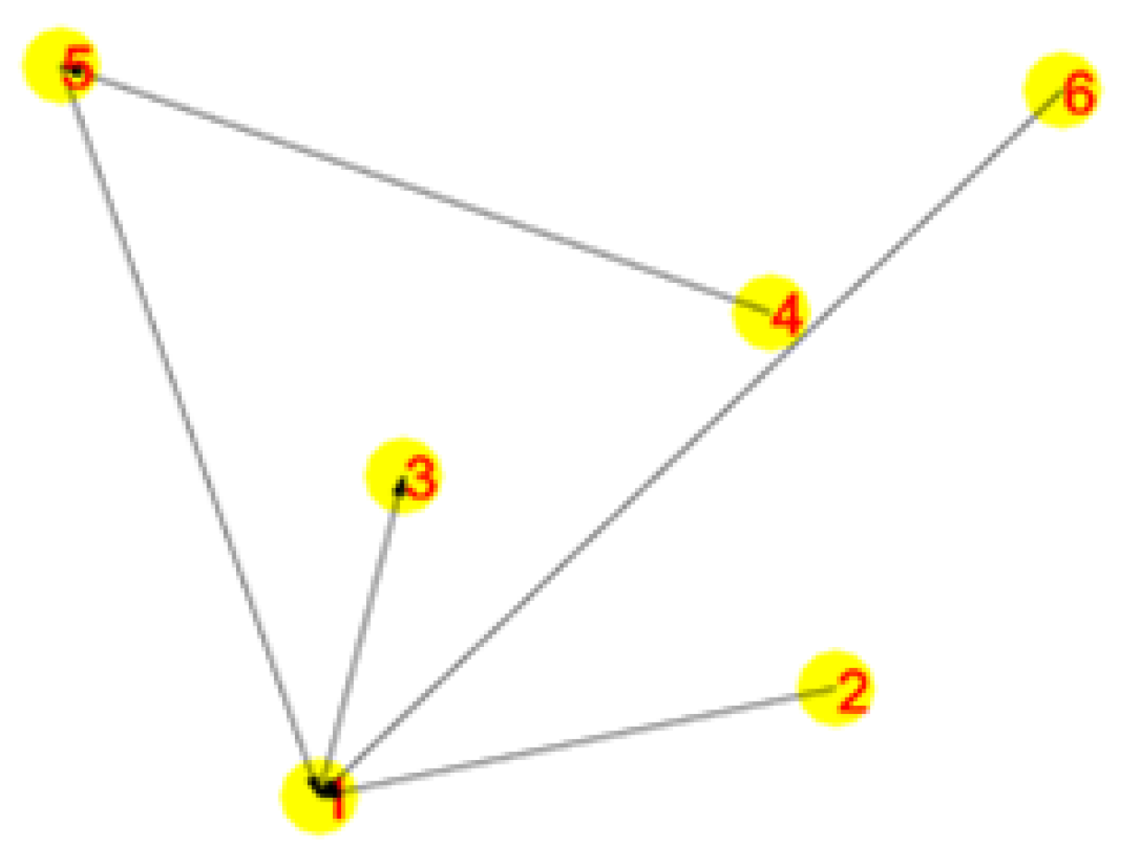
According to the fast modularity optimization method and the task execution sequence of likewise products in the product reference library, Meta tasks are optimized with the principle of “high cohesion, low coupling”, and the information exchange relationship between cloud tasks will be established through the expert evaluation method. Finally, we use a weighted, undirected graph to represent the task relationship between the meta-tasks, and establish the adjacency matrix W to generate the directed graph (Figure 6).
First, according to the established adjacency matrix, we generate the graph community and calculate the modularity M of the original graph structure. Then we regard the meta-task as a kind of graph group, and aggregate any two graph groups. Calculate the degree of modularity after aggregation, take the two graph groups with the largest value-added to aggregate, and continuously calculate the increment of modularity. Repeat the above algorithm until the increase in modularity is over, we can achieve the best aggregation. The result of meta-task clustering graph is shown in Figure 7.
With reference to the decomposition granularity of similar tasks in the product library, we set the average task granularity of the reference task as the task granularity measurement threshold and set it to 0.5832. Calculate the average value of subtask’s granularity in the subtask aggregation result, and compare with the threshold value of the overall the CMfg task granularity measurement. We can judge by Equation (31).
The task granularity measurement of the task decomposition aggregation scheme is within the threshold, which certifies that the task granularity of the aggregation result meets the requirements. Meanwhile, we found task correlation between the split points of the task undirected graph is low, in which the coupling between tasks is weak. The results demonstrate the rationality of graph segmentation.
5.3. Transportation Task Simulation
We take the transportation task that composed of 6 consecutive subtasks as an example. The customer can set parameter values according to their needs. We set the maximum number of iterations to 100, the number of hired bees to 20, the number of observation bees to 20, limit to 50, to 560, to 450, to 80, and to 40. With the consideration of actual processing requirements, we take transportation cost, transportation quality, and transportation time as the main consideration indicator, and transportation capacity as the secondary consideration indicators. Manufacturing resources are diversified in the CMfg environment. The same resource requirements may have different degrees of importance to the same indicators. Considering the comprehensive evaluation index should meet the actual transportation environment requirements, we use the AHP method to obtain the weight value in three situations. The first situation is that transportation cost is the most important, transportation time is second, and transportation quality is more important than transportation capacity, namely . The second situation is that transportation quality is the most important, transportation time is second, transportation cost is more important than transportation capacity, namely . The third type situation that transportation time is the most important, transportation cost is second, transportation quality is more important than transportation capacity, namely . When the transportation time is the most important we use the AHP method to construct the judgment matrix . The details are shown in Table 4.
According to the AHP method, we find the weight of each indicator, : (0.53228780, 0.25375611, 0.15579803, 0.05815806). Where is the weight factor of manufacturing resources in CMfg. However, the weight also needs the consistency test to determine. With the Equation (28), we find the maximum characteristic root: . With the Equation (29), We find the calculated consistency index value: . Find the average random consistency index, and attain the results that according to Equation (30) are in Table 5. We compare them and produce the result, . In the same way, we obtain the first case and the second case, respectively, as shown in Table 5. We calculate fitness function in various situations through artificial bee colony algorithm in Section 4.3. Then, we design simulation experiments fitness value comparison curve, and comparison results are shown in Figure 8.
The simulation results show that the objective function value is the smallest when the transportation time is the most important, which means we can choose to attain the optimal transportation task decomposition plan. At the same time, we found that the algorithm can achieve convergence less than 20 episodes, which proves that our algorithm has excellent characteristics in solving transportation task decomposition.
5.4. Maintenance Task Simulation
Industrial robots are the device in the intelligent production line of workshop. Like other equipment, it may broke down when put into production, so it is necessary to carry out regular maintenance on industrial robots. Regular maintenance can effectively reduce the probability of failure and improve production efficiency while ensuring the service life of industrial robots. We input the working hours and working years of robots into the system. Use the normal maintenance time nodes of 1000 h, 20,000 h, and 30,000 h as the standard, and evaluate the equipment loss through CMfg platform. Finally, the platform system gives the corresponding decomposition results according to the input information in Table 6. Machines 1, 2, 5, 16, and 19 need minor revise, we select resources with service capability and service reputation of level 2 or higher in area 1. Machines 3, 10, and 17 need middle revise, we select resources with service capability and service reputation of level 3 in area 2. Machine 11 need major revise, and we select resources with service capability and service reputation of level 3 in area 1. Machine 11 need specialized revise, we select resources with service capability and service reputation of level 2 or higher in area 2.
From the above optimal task decomposition scheme, we can effectively decompose tasks according to requirements at each stage. The stages are both interconnected and independent to each other, which satisfies the requirements of the cloud platform for task decomposition. Therefore, the method proposed in this paper can effectively obtain the optimal results, which is suitable for complex tasks decomposition in CMfg.
6. Conclusions
There are large-scale manufacturing resources and highly complex tasks in CMfg, the high efficiency task decomposition method was desirable. In this paper, a task decomposition system structure based on cloud platform, for addressing complex asymmetric task decomposition problems in CMfg, is presented. With the consideration of the characteristics of product lifecycle and relationships, the research divided the production process into four stages: design, manufacturing, transportation, and maintenance. This problem is transformed into a multi-stage optimization decomposition problem that the complexity of task decomposition was reduced.
The paper has proposed a complex task decomposition model based on a cloud platform. In the design task model, the concept of correlation coupling degree is introduced to ensure high independence between subtask modules. Through the deep-first search algorithm, the problem of complex design task decomposition is transformed into a Boolean matrix decomposition and search problem. The complexity of the problem reduced too much by the algorithm. The production attributes of manufacturing task mostly are modular collaborative work. By using fast modular optimization algorithm, the task is decomposed into different subtask modules that was the optimal manufacturing sequence. The transportation with criteria time, quality, cost, and transport capacity was introduced in the model. We use artificial bee colony algorithm to produce an optimal transportation plan, and the result demonstrate transportation time need a higher priority. Maintenance tasks are mostly overlooked in production processes, we developed a cloud task formal description system according to basic information, attribute information, and service information. Meanwhile, a cloud platform can find a maintenance plan by the task description of the cloud task. Through the above study, we proposed a task decomposition frame based cloud platform, and a hybrid method was used to address multi-stage task decomposition problem. Finally, a case study of workshop intelligent production line was presented to demonstrate efficiency and accuracy of the model and method proposed in CMfg.
In future work, study on judgment standards for different tasks in the maintenance process is required, and comprehensive evaluation index of cloud manufacturing task decomposition is also important. In addition, with high scalability, the proposed hybrid method can be applied to multi-stage combinatorial optimization problem (e.g., vehicle manufacturing, steelmaking-continuous, and wafers manufacturing) in CMfg. The parameters setting and operators’ improvement of the method still requires further research.
Author Contributions
Conceptualization, Y.H.; methodology, J.W.; software, Z.Z.; validation, Z.Z., J.W., and Z.W.; formal analysis, H.L.; investigation, Z.W.; resources, J.W.; data curation, Y.H.; writing—original draft preparation, Z.Z.; writing—review and editing, Z.Z.; visualization, Y.H.; supervision, Z.Z.; project administration, Y.H.; funding acquisition, Y.H. All authors have read and agreed to the published version of the manuscript.
Funding
This research received no external funding.
Institutional Review Board Statement
Not applicable.
Informed Consent Statement
Not applicable.
Data Availability Statement
Not applicable.
Acknowledgments
This research work was supported by the Education Department Project of Jilin Province, no. JJKH20200659KJ and JJKH20181033KJ.
Conflicts of Interest
The authors declare no conflict of interest.
References
- Tao, F.; Hu, Y.F.; Zhou, Z.D. Study on manufacturing grid & its resource service optimal-selection system. Int. J. Adv. Manuf. Technol. 2008, 37, 1022–1041. [Google Scholar]
- Radu, L.D. Green cloud computing: A literature survey. Symmetry 2017, 9, 295. [Google Scholar] [CrossRef] [Green Version]
- Tao, F.; Zuo, Y.; Da, X.L.; Zhang, L. IoT-based intelligent perception and access of manufacturing resource toward cloud manufacturing. IEEE Trans. Ind. Inform. 2014, 10, 1547–1557. [Google Scholar]
- Valilai, O.F.; Houshmand, M.A. A collaborative and integrated platform to support distributed manufacturing system using a service-oriented approach based on cloud computing paradigm. Robot. Comput. Integr. Manuf. 2013, 29, 110–127. [Google Scholar] [CrossRef]
- Leng, J.; Yan, D.; Liu, Q.; Xu, K.; Zhao, J.L.; Shi, R.; Wei, L.; Zhang, D.; Chen, X. ManuChain: Combining Permissioned Blockchain With a Holistic Optimization Model as Bi-Level Intelligence for Smart Manufacturing. IEEE Trans. Syst. Man Cybern. Syst. 2020, 50, 182–192. [Google Scholar] [CrossRef]
- Leng, J.; Ye, S.; Zhou, M.; Zhao, J.L.; Liu, Q.; Guo, W.; Cao, W.; Fu, L. Blockchain-secured smart manufacturing in industry 4.0: A survey. IEEE Trans. Syst. Man Cybern. Syst. 2020, 51, 237–252. [Google Scholar] [CrossRef]
- Wu, D.; Greer, M.J.; Rosen, D.W.; Schaefer, D. Cloud manufacturing: Strategic vision and state-of-the-art. J. Manuf. Syst. 2013, 32, 564–579. [Google Scholar] [CrossRef] [Green Version]
- Wang, Y.; Cheng, L. Event-driven cloud dynamic task decomposition mode optimization method. Syst. Simul. J. 2018, 30, 4029–4042. [Google Scholar]
- Yu, L.S.; Jiang, Z.B.; Liu, K. Research on task decomposition and state abstraction in reinforcement learning. Artif. Intell. Rev. 2012, 38, 119–127. [Google Scholar]
- Zhou, K.; Lu, M.; Wang, G.; Ren, B.Y. Manufacturing task decomposition and collaborative optimization of manufacturing cell-level resource allocation. Hal J. Bin Inst. Technol. 2009, 41, 47–52. [Google Scholar]
- Weiss, B.A.; Sharp, M.; Klinger, A. Developing a hierarchical decomposition methodology to increase manufacturing process and equipment health awareness. J. Manuf. Syst. 2018, 48, 96–107. [Google Scholar] [CrossRef] [PubMed]
- Garashcheko, Y.; Rucki, M. Part decomposition efficiency expectation evaluation in additive manufacturing process planning. Int. J. Prod. Res. 2020. [Google Scholar] [CrossRef]
- Dikici, A.; Turetken, O.; Demirors, O. Factors influencing the understandability of process models: A systematic literature review. Inf. Softw. Technol. 2018, 93, 112–129. [Google Scholar] [CrossRef] [Green Version]
- Liu, M.Z.; Wang, Q.; Ling, L. Cloud manufacturing task decomposition method based on hierarchical task network. China Mech. Eng. 2017, 28, 924–930. [Google Scholar]
- Guo, L.; Xu, Y.; He, W.; Cheng, Y.X. Optimization of complex part-machining services based on feature decomposition in cloud manufacturing. Int. J. Comput. Integr. Manuf. 2020, 33, 1227–1244. [Google Scholar] [CrossRef]
- Zhang, Z.; Zhang, Y.; Lu, J.; Gao, F.; Xiao, G. A novel complex manufacturing business process decomposition approach in cloud manufacturing. Comput. Ind. Eng. 2020, 144, 106442. [Google Scholar] [CrossRef]
- Liu, N.; Li, X.; Shen, W. Multi-granularity resource virtualization and sharing strategies in cloud manufacturing. J. Netw. Comput. Appl. 2014, 46, 72–82. [Google Scholar] [CrossRef]
- Georgievski, I.; Alillo, M. HTN planning: Overview, comparison, and beyond. Artif. Intell. 2015, 222, 124–156. [Google Scholar] [CrossRef]
- Zhou, L.; Zhang, L.; Fang, Y. Logistics service scheduling with manufacturing provider selection in cloud manufacturing. Robot. Comput. Integr. Manuf. 2020, 65, 101914. [Google Scholar] [CrossRef]
- Blondel, V.D.; Guillaume, J.L.; Lambiotte, R.; Lefebvre, E. Fast unfolding of communities in large networks. J. Stat. Mech. Theory Exp. 2008, 2008, P10008. [Google Scholar] [CrossRef] [Green Version]
- Karaboga, D.; Ozturk, C. A novel clustering approach: Artificial Bee Colony (ABC) algorithm. Appl. Soft Comput. 2011, 11, 652–657. [Google Scholar] [CrossRef]
Figure 1.
Product lifecycle.

Figure 2.
Task constraint structure.

Figure 3.
Task attribute index.

Figure 4.
Artificial bee colony algorithm process.

Figure 5.
The structure of task tree.

Figure 6.
Meta-task relation directed graph.

Figure 7.
Meta-task clustering graph.

Figure 8.
The convergence diagrams when weights are transportation time, transportation cost, and transportation quality are the most important.
Figure 8.
The convergence diagrams when weights are transportation time, transportation cost, and transportation quality are the most important.


Table 1.
Maintenance task indicators.
| Criteria | Detailed Research Contents |
|---|---|
| Time (T) | Maintenance time of resource in CMfg |
| Waste (W) | The degree of equipment waste under different working conditions |
| District (D) | The district that the maintenance task issuer serves to the service resource customer |
| Ability (B) | Maintenance service execution efficiency |
| Credit (C) | Recognition of the credit of service resources by the issuer of the maintenance task |
Table 2.
Average stochastic index RI.
| RI | 0.00 | 0.58 | 0.90 | 1.12 | 1.24 | 1.32 | 1.41 | 1.46 | 1.49 |
Table 3.
Meta-task based information.
| Task Number | Task Name | Task Number | Task Name |
|---|---|---|---|
| 1 | Welding robot chassis | 25 | Reclaiming robot effector |
| 2 | Welding robot joint Ⅰ | 26 | Reclaiming robot reducer |
| 3 | Welding robot shoulder | 27 | Reclaiming robot servo motor |
| 4 | Welding robot arm | 28 | Reclaiming robot controller |
| 5 | Welding robot elbow | 29 | Cutting robot chassis |
| 6 | Welding robot joint Ⅱ | 30 | Cutting robot waist |
| 7 | Welding robot forearm | 31 | Cutting robot upper arm |
| 8 | Welding robot wrist | 32 | Cutting robot lower arm |
| 9 | Welding robot end effector | 33 | Cutting robot joint |
| 10 | Welding robot reducer | 34 | Cutting robot wrist |
| 11 | Welding robot servo motor | 35 | Cutting robot actuator |
| 12 | Welding robot controller | 36 | Cutting robot reducer |
| 13 | Handling robot chassis | 37 | Cutting robot servo motor |
| 14 | Handling robot waist | 38 | Cutting robot controller |
| 15 | Handling robot arm | 39 | Painting robot chassis |
| 16 | Handling robot wrist | 40 | Painting robot waist |
| 17 | Handling robot actuator | 41 | Painting robot upper arm |
| 18 | Handling robot brake | 42 | Painting robot lower arm |
| 19 | Handling robot controller | 43 | Painting robot wrist |
| 20 | Reclaiming robot chassis | 44 | Painting robot actuator |
| 21 | Reclaiming robot waist | 45 | Painting robot reducer |
| 22 | Reclaiming robot upper arm | 46 | Painting robot servo motor |
| 23 | Reclaiming robot lower arm | 47 | Bearing structure |
| 24 | Reclaiming robot wrist | 48 | Assembly inspection |
Table 4.
Weight index.
| T | C | Q | Tr | |
|---|---|---|---|---|
| T | 1 | 3 | 3 | 7 |
| C | 1/3 | 1 | 2 | 5 |
| Q | 1/3 | 1/2 | 1 | 3 |
| Tr | 1/7 | 1/5 | 1/3 | 1 |
Table 5.
The normalized weight values when transportation cost, quality, and time are the most important.
Table 5.
The normalized weight values when transportation cost, quality, and time are the most important.
| Time | Transportation Cost | Transport Quality | Transport Capacity | |
|---|---|---|---|---|
| T > C > Q > Tr | 0.53228780 | 0.25375611 | 0.15579803 | 0.05815806 |
| C > T > Q > Tr | 0.55549672 | 0.24587890 | 0.14135998 | 0.05726439 |
| Q > T > C > Tr | 0.49777984 | 0.30382881 | 0.13209338 | 0.06629797 |
Table 6.
Resource wastage state.
| Resources | Hours | Loss Degree | District | Abilities | Credit |
|---|---|---|---|---|---|
| 1 | 1530 | 5 | 1 | 2 | 2 |
| 2 | 2530 | 4 | 1 | 2 | 2 |
| 3 | 20,300 | 8 | 2 | 3 | 3 |
| 4 | 800 | 2 | 1 | 2 | 2 |
| 5 | 1340 | 2 | 1 | 2 | 3 |
| 6 | 3002 | 2 | 2 | 3 | 2 |
| 7 | 900 | 1 | 2 | 2 | 2 |
| 8 | 725 | 2 | 2 | 1 | 1 |
| 9 | 1560 | 2 | 1 | 3 | 3 |
| 10 | 21,050 | 8 | 2 | 3 | 3 |
| 11 | 34,000 | 9 | 1 | 3 | 3 |
| 12 | 500 | 1 | 2 | 3 | 2 |
| 13 | 400 | 1 | 1 | 1 | 2 |
| 14 | 3050 | 2 | 2 | 2 | 3 |
| 15 | 800 | 1 | 2 | 2 | 3 |
| 16 | 1800 | 1 | 2 | 2 | 2 |
| 17 | 25,600 | 8 | 2 | 3 | 3 |
| 18 | 950 | 1 | 2 | 2 | 2 |
| 19 | 1120 | 5 | 1 | 2 | 2 |
| 20 | 600 | 1 | 1 | 2 | 2 |
Publisher’s Note: MDPI stays neutral with regard to jurisdictional claims in published maps and institutional affiliations. |
© 2021 by the authors. Licensee MDPI, Basel, Switzerland. This article is an open access article distributed under the terms and conditions of the Creative Commons Attribution (CC BY) license (https://creativecommons.org/licenses/by/4.0/).
Share and Cite
MDPI and ACS Style
Hu, Y.; Zhang, Z.; Wang, J.; Wang, Z.; Liu, H. Task Decomposition Based on Cloud Manufacturing Platform. Symmetry 2021, 13, 1311. https://0-doi-org.brum.beds.ac.uk/10.3390/sym13081311
AMA Style
Hu Y, Zhang Z, Wang J, Wang Z, Liu H. Task Decomposition Based on Cloud Manufacturing Platform. Symmetry. 2021; 13(8):1311. https://0-doi-org.brum.beds.ac.uk/10.3390/sym13081311
Chicago/Turabian StyleHu, Yanjuan, Ziyu Zhang, Jinwu Wang, Zhanli Wang, and Hongliang Liu. 2021. "Task Decomposition Based on Cloud Manufacturing Platform" Symmetry 13, no. 8: 1311. https://0-doi-org.brum.beds.ac.uk/10.3390/sym13081311
Note that from the first issue of 2016, this journal uses article numbers instead of page numbers. See further details here.