
A Multiple Comprehensive Analysis of scATAC-seq Based on Auto-Encoder and Matrix Decomposition

1
College of Chemistry, Sichuan University, Chengdu 610064, China
2
School of Cyber Science and Engineering, Sichuan University, Chengdu 610065, China
*
Authors to whom correspondence should be addressed.
Symmetry 2021, 13(8), 1467; https://0-doi-org.brum.beds.ac.uk/10.3390/sym13081467
Submission received: 10 June 2021
/
Revised: 4 August 2021
/
Accepted: 7 August 2021
/
Published: 11 August 2021
(This article belongs to the Special Issue Research on Symmetry in Chemometrics)
Abstract
:Single-cell ATAC-seq (scATAC-seq), as the updating of ATAC-seq, provides a novel method for probing open chromatin sites. Currently, research of scATAC-seq is faced with the problem of high dimensionality and the inherent sparsity of the generated data. Recently, several works proposed the use of an autoencoder–decoder, a symmetry neural network architecture, and non-negative matrix factorization methods to characterize the high-dimensional data. To evaluate the performance of multiple methods, in this work, we performed a multiple comparison for characterizing scATAC-seq based on four kinds of auto-encoders known as a symmetry neural network, and two kinds of matrix factorization methods. Different sizes of latent features were used to generate the UMAP plots and for further K-means clustering. Using a gold-standard data set, we practically explored the performance among the methods and the number of latent features in a comprehensive way. Finally, we briefly discuss the underlying difficulties and future directions for scATAC-seq characterizing. As a result, the method designed for handling the sparsity outperforms other tools in the generated dataset.
1. Introduction
The assay for transposase-accessible chromatin using sequencing (ATAC-seq) is an efficient method to detect open chromatin sites in the whole genome, which tags genomes with sequencing adaptors using Tn5 transposase [1]. Recently, single-cell sequencing technology, such as single-cell approaches for the assay for transposase-accessible chromatin using sequencing (scATAC-seq) [2,3], has developed rapidly, which can reveal the variations of chromatin accessibility at the single-cell level. With the emergence of thousands of single-cell chromatin accessibility analysis methods, scATAC-seq has rapidly become one of the preferred methods for single-cell applications [4]. However, datasets generated by this technology are difficult to analyze because of the high dimensionality and the inherent sparsity.
As for scRNA-seq, many tools such as Seurat [5], Scanpy [6] and Monocle [7] have been widely used, but the analysis tools of scATAC-seq data are relatively new. Some existing tools contribute to some aspects of scATAC-seq analysis, such as SnapATAC [8], Scasat [9], cisTopic [10], scABC [11] and scATAC-pro [12], but the analysis of scATAC-seq still has a lot to explore.
Moreover, as a powerful symmetry neural network, deep generative models have been used to analyze scRNA-seq. Currently, a popular method is a variational autoencoder (VAE), which estimates the data distribution through a symmetry neural network composed of encoder and decoder and learns the latent feature from the input data [13]. Recently, Romain Lopez et al. developed scVI, a neural network mapping the latent features to the ZINB distribution, adapting VAE for scRNA-seq analysis [14]. Soon after, Lei Xiong et al. applied VAE to scATAC-seq analysis and provided SCALE which combined a generative network and a probabilistic Gaussian Mixture Model to learn latent features from scATAC-seq data [15]. The Gaussian mixture model (GMM), as a priori of potential characteristic variables (latent feature), is used for unsupervised clustering by learning more interpretable potential representations [16]. Moreover, Yingxin Cao et al. provided SAILER, which used the traditional encoder–decoder framework to learn the potential representation but imposes additional constraints to ensure that the learned representation is independent of confounding factors [17]. However, VAE is mainly due to its architectural affinity with basic automatic coders, although their mathematical formulas are significantly different. The basic autoencoder is a symmetric neural network, which is used to learn the coding of effective data unsupervised [18]. Moreover, the variants of autoencoder methods were provided to make the learned latent features contain more information [19]. For example, the sparse autoencoder [20,21] added the sparsity constraint by extending the Kullback–Leibler (KL) divergence so that the model can respond to the unique statistical characteristics of training data. As a widely used deep learning technology, the stacked autoencoder has been researched as a common component of DNN by Bengio et al. [22].
Matrix factorization is also used in high-dimensional genomic sequencing data. Chunxuan Shao et al. used non-negative matrix factorization (NMF) for scRNA-seq analysis and their results show that NMF is a robust, informative and simple method, which can learn cell subtypes from single cell gene expression data unsupervised [23].
The autoencoders are important approaches for measuring the performance of analyzing high-dimensional and sparse genomic sequencing data, but currently, no study has examined the performance globally. Therefore, we performed a comparison for analyzing scATAC-seq based on four kinds of autoencoders known as a symmetry neural network, and two kinds of matrix factorization methods. Finally, we found that all types of cells except EXs can be well separated. For EX cells, more effective methods are needed to separate them. These results would be helpful for the related research which needs a selection strategy of high-dimensional and extremely sparse data processing. The code in this work is available with MIT license in https://github.com/jingry/scATACCharacterization (accessed on 30 July 2021).
2. Materials and Methods
The workflow is shown in Figure 1. Four kinds of neural networks and two kinds of matrix factorization were used to reduce dimension. The low-dimensional variables obtained after dimensionality reduction are “latent features”. Uniform Manifold Approximation and Projection (UMAP) was used to embed the latent features to 2 dimensions and K-means clustered on the extracted low dimensional potential variables to obtain cluster assignments.
2.1. Dataset
The publicly available Forebrain dataset we used is derived from P56 mouse forebrain cells [24]: forebrain tissue of 8-week-old adult mice (56th day after birth) and mouse embryos at 7 developmental stages from embryonic day 11.5 to birth. The forebrain dataset can be accessed at GSE100033. The number of cells (i.e., samples) is 2088 and the dimension of the dataset (i.e., features) is 11,285. It contains eight cell types: the eight developmental stages of the mouse forebrain. The first part: EX (i.e., EX1, EX2, EX3); the EX represents the excitatory neurons. The second part is the IN which represents inhibitory neurons (i.e., IN1, IN2). The other parts are AC: astrocyte, OC: oligodendrocyte and MG: microglia. EX1 and EX3 are more similar to the upper and lower cortical layers. EX2 has the characteristics of dentate gyrus neurons [24]. The cell type is the label that we use for clustering. We filtered the scATAC-seq count matrix similar to SCALE, retaining only 10 cells with a peak of ≥2 reads and removed rare peaks with reads of > 2 in less than X% of cells. The ubiquitous peaks (reads ≥ 1 in at least (100 − X)% of cells) were also removed [15]. By default, X is 6. The reason of the count matrix filter is that ubiquitous and rare peaks are often not informative for clustering.
2.2. Feature Representation
In general, using manifold methods for exploring the latent relations from the encoded information has been widely used in many deep learning works. In our model, the Python package “UMAP” was used to embed the encoded latent information to 2-dimensional data for plotting. Uniform Manifold Approximation and Projection (UMAP) [25] is a dimension reduction technique always used for visualization which is similarly to t-distributed stochastic neighbor embedding (t-SNE) [26].
2.3. Auto-Encoders
The input scATAC-seq data is (n peaks), with indicating whether there is a peak or not in bin . depends on experimental confounding factors and the inherent characteristics of cells. We aim to obtain a potential representation of (i.e., embedded) for each cell which reflects its properties. Additionally, we let be this potential variable (i.e., latent feature). Matrix was the input used for each kind of autoencoder and extracted the latent feature . We set the dimension of the latent feature for as 10 in our analysis. In contrast, we also set the case of the dimension of the latent feature as 20.
Datasets arising from scATAC-seq technology are difficult to analyze due to the high dimensionality and the inherent sparsity. However, the symmetry neural network (autoencoder) is good at processing high-dimensional data. In this work, four autoencoders are used for encoding the scATAC-seq data.
All the neural networks in the autoencoders are implemented with the “pytorch” [27] framework in Python. The number of iterations (epochs) was set as 10,000 because after the number of epochs, the result changes only a little. Adam optimizer [28] using minibatch training and with weight decay 5 × 10⁻⁴ is used to optimize the General autoencoder, Sparse autoencoder and Variational autoencoder. Additionally, SGD optimizer is used to optimize the Stacked autoencoder. The detailed descriptions of the autoencoders and the brief introduction of the autoencoders’ structurse used in this work are listed in Table 1.
2.3.1. General Autoencoder
A general autoencoder is an artificial neural network which is used to learn effective data coding in an unsupervised way [18]. A general autoencoder is an unsupervised learning algorithm, which sets the target value equal to input value. The aim of a general autoencoder is to learn the potential variable (latent features) for the input data, and it is usually used for dimensionality reduction. The autoencoder is applied to many situations, such as face recognition [29], obtaining the semantics of words [30] and is now also used in single-cell seq analysis.
2.3.2. Sparse Autoencoder
A sparse autoencoder’s training criterion involves the sparsity penalty of the code layer. The sparsity constraint forces the neural network to respond to the unique statistical characteristics of input data. The sparsity penalty value is the characteristic of sparse autoencoder. Other algorithms used in this work do not consider the penalty value for sparsity. Sparsity can be obtained by using the penalty term of Kullback–Leibler (KL) divergence [20,21]. Additionally, KL divergence is a standard function to measure two different distributions [21]. KL divergence is used in loss function calculations.
2.3.3. Stacked Autoencoder
A stacked autoencoder, investigated as a common component of DNN [22], is composed of several layers of autoencoders. The output of the previous hidden layer is connected to the input of the next hidden layers. Stacked autoencoders contain three steps [31]:
- Use the input data to train the autoencoder and obtain the learning data.
- Take the learning data of the previous hidden layer as the input of the next hidden layer until the end of training.
- After training all hidden layers, the backpropagation algorithm is used to minimize the cost function, and the training set is used to update the weights to achieve fine-tuning.
2.3.4. Variational Autoencoder
Variational autoencoders (VAEs) [32] are generative neural networks, and VAEs are similar to generative adversarial networks [33]. VAEs can estimate the distribution of data through the encoder and decoder and learn the potential features from the input data. The method maximizes the similarity between the calibration data and the input data and minimizes the Kullback–Leibler (KL) divergence between the approximate value and the true a posteriori value [13]. The VAE model relies on assumptions about the distribution of latent features. It uses a variational method for potential representation learning using a specified loss function (such as KL divergence) and an estimator (such as Stochastic Gradient Variational Bayes) [13]. VAE models the input matrix through a generative process. In the encoder part, the corresponding latent features can be obtained through the encoder via the reparameterization. In the decoder part, the sample can be generated through the decoder. Moreover, it applies Gaussian Mixture Model (GMM) as the prior over the latent features [34]; the GMM model is used to initialize the parameters and . (mean) and (variance) are learned by the encoder network from the input matrix. Each cell is first transformed into latent features on the GMM by an encoder network and then reconstructed through a decoder network. In this work, GMM models are achieved by the “scikit-learn” package of Python. The neural network is implemented by the “pytorch” package.
2.4. Matrix Factorization
As an alternative approach, using matrix factorization could reduce the dimension of data as well. Practically, matrix factorization algorithms work by decomposing the matrix into two lower dimensionality matrices [35]. Matrix factorization not only can be used to dimension reduction directly but can also be used for feature purification. Both NMF and Lsnmf used in this work belong to matrix factorization.
2.4.1. Non-Negative Matrix Factorization (NMF)
Non-negative matrix factorization (NMF) is a set of dimensionality reduction algorithms in multivariate analysis and linear algebra [36]. NMF can used in in missing data imputation [37], chemometrics and bioinformatics [38]. NMF [39], as a decomposition method, assumes that the input matrix and the component part are non-negative. NMF decomposes the nonnegative matrix (V) into a basis matrix (W) and a coefficient matrix (H) (Equation (1)). The basis matrix (W) was used for analysis in this work. When carefully constrained, NMF can generate a representation-based part of the dataset to generate an interpretable model [40]. In this work, the “NMF” method is from the Python “scikitlearn” package.
2.4.2. Alternating Non-Negative Least Squares Matrix Factorization (Lsnmf)
Nimfa [41], an open-source library in Python, provides a uniform interface for non-negative matrix decomposition algorithms. Lsnmf is a package in Nimfa, and the projection gradient (constrained optimization) method is used for each subproblem [42]. The algorithm converges faster than the popular multiplication update method and it depends on the effective solution of the bounded bundle subproblem. Similarly to NMF, Lsnmf also decomposes the input nonnegative matrix (V) into a basis matrix (W) and a coefficient matrix (H). The Lsnmf algorithm retains the advantages of the original NMF algorithm, which is easy to implement and ensures the local optimal solution, but improves the performance of connecting function-related genes [43].
2.5. Clustering
Additionally, the K-means clustering method was employed to separate the samples into the clusters by using the “scikitlearn” package. K-means clusters data by separating samples into n groups of equal variance and minimizes the criterion called inertia [44]. In this work, we applied K-means clustering on the latent features to obtain cluster assignments, which were used to estimate the clustering accuracy.
2.6. Performance Evaluation of Clustering
The clustering accuracy was assessed by evaluation matrices between cluster assignments predicted by K-means and the reference cell types. The adjusted Rand index (ARI), normalized mutual information (NMI), F1 score and Silhouette_score were used to compare clustering results of each method.
2.6.1. Adjusted Rand Index (ARI)
The Adjusted Rand Index (ARI) was used to evaluate the clustering results by Equation (2). The larger the value, the more realistic the clustering results are.
The Rand Index (RI) calculates the similarity measure between two clusters. E (RI) is the expected value of the Rand Index. The ARI can be represented by Equation (3) when the contingency table is given [45].
2.6.2. Normalized Mutual Information (NMI)
Normalized Mutual Information (NMI) is a normalization of the Mutual Information (MI) score to scale the results between 0 and 1. Zero represents no mutual information and 1 represents perfect correlation.
P, T, I and H represent the clustered label, the real label, the mutual entropy and the Shannon entropy, respectively.
2.6.3. F1 Score
The F1 score can be regarded as a weighted average of model accuracy and recall; its best value at 1 and worst score at 0. The formula is Equation (5).
2.6.4. Silhouette_Score
The Silhouette Coefficient is calculated using the mean intra-cluster distance () and the mean nearest-cluster distance () for sample. The best value is 1 and the worst value is −1. Values near 0 indicate overlapping clusters. Negative values generally indicate that a sample has been assigned to the wrong cluster, as a different cluster is more similar. The formula of Silhouette Coefficient is Equation (6).
3. Results
Four kinds of autoencoder and two matrix factorization methods were used for extracting features from scATAC-seq. For each method, we tested the number of latent features from 8 to 128 (8, 16, 32, 64 and 128). The results of each case are listed in Supplementary Figures S1–S30 and Supplementary Tables S1–S6.
- The General autoencoder was used for dimensionality reduction of scATAC-seq and the K-means clustering was applied on the extracted latent features to obtain cluster assignments, and the cluster assignments were used to assess the clustering accuracy. Then, the extracted features were visualized with UMAP.
- The Sparse autoencoder (SparseAE), an autoencoder whose training criterion involves a sparsity penalty on the code layer, was used for dimensionality reduction of scATAC-seq. K-means clustering was applied on the extracted latent features to obtain cluster assignments. The cluster assignments were used to assess the clustering accuracy. In the end, the extracted features were visualized with UMAP.
- Stacked autoencoder (StackedAE) is a neural network which consists of several layers of autoencoders where the output of each hidden layer is connected to the input of the successive hidden layer. It was used for dimensionality reduction of scATAC-seq. K-means clustering was applied on the extracted latent features to obtain cluster assignments and the extracted features were visualized with UMAP.
- Variational autoencoders (VAEs) are generative models similar to generative adversarial networks. In this work, they were used for dimensionality reduction of scATAC-seq. K-means clustering was applied on the extracted latent features to obtain cluster assignments and the extracted features were visualized with UMAP.
- Non-negative Matrix Factorization (NMF), a traditional machine learning method, was also used for the dimensionality reduction of scATAC-seq. K-means and UMAP were used in the same way as above.
- Alternating Non-negative Least Squares Matrix Factorization (Lsnmf)—the calculation flow of Lsnmf is the same as that of NMF.
We made a multiple comparison based on the feature embedding and cluster assignments. In general, 13 neural networks and four machine learning models were provided. Moreover, the extracted features used for clustering by K-means and evaluation metrics of clustering are F1 score, Adjusted Rand Index (ARI), Normalized Mutual Information (NMI) and Silhouette_score.
3.1. General Autoencoder
The general autoencoder was used for dimensionality reduction of scATAC-seq. Feature embedding and evaluation matrices are shown in Figure 2 with different numbers of latent features. From the UMAP plot, reducing dimension to 20 seems to have more obvious separation of cell types than 10 latent features (Figure 2a,c). However, the cluster results of 10 latent features and 20 latent features were similar (Figure 2b,d and Table 2).
The General autoencoder was also used to reduce dimensions to different numbers of latent features. The feature embedding and evaluation matrices are listed in Figure 3. We can find that there will be a critical point for the number of latent features. When the dimension number has reduced to a certain extent, the dimension number has little effect. With the number of latent feature dimension, 8, 16, 32, 64 and 128, the results using the General autoencoder are roughly similar. The details of evaluation metrics and plot of feature embedding were listed in Supplementary Figures S1–S5 and Supplementary Table S1. When the number of latent features continues to increase, such as to 64 latent features, the results are worse. The F1 score, ARI and NMI with the 64 latent features are 0.32, 0.140 and 0.290. The F1 score, ARI and NMI with the 128 latent features are 0.21, 0.017 and 0.063.
3.2. Sparse Autoencoder (SparseAE)
The Sparse autoencoder was used for the dimensionality reduction of scATAC-seq. The Feature embedding and evaluation matrices of the embedded layer with 10 latent features and 20 features are shown in Figure 4. The Dimensionality reduction efficiency of SparseAE is relatively good. EX1, EX2 and EX3, three clusters of excitatory neuron cells, are close to each other in the UMAP plot (Figure 4). Apart from EX1, EX2 and EX3, other parts can be clearly separated. The F1 score, ARI, NMI and Silhouette_score of the embedded layer with 10 latent features using SparseAE are 0.71, 0.499, 0.584 and 0.065.
The F1 score, ARI, NMI and Silhouette_score of the embedded layer with 20 latent features using SparseAE are 0.67, 0.481 0.571 and 0.056 (Table 2).
Although SparseAE cannot be a deep neural network, the result is still better because of the sparsity constraint. In this work, there is only one hidden layer with “ReLU” activation function and KL divergence is a part of loss calculation which makes the model more effective.
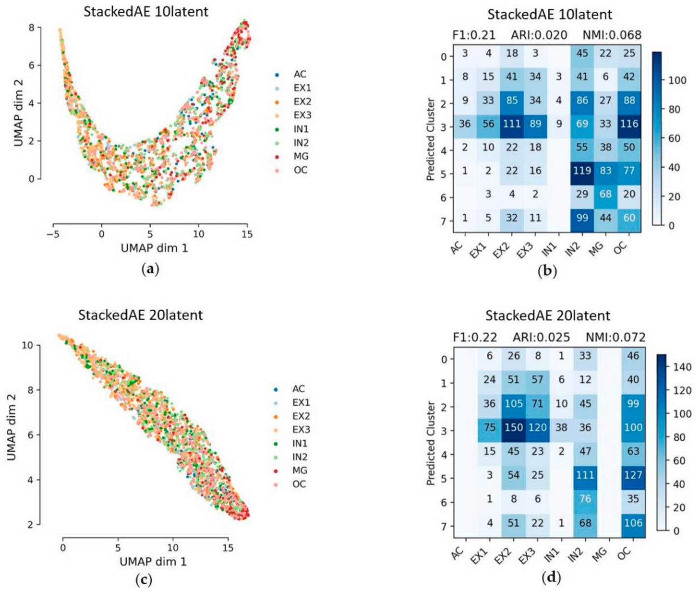
3.3. Stacked Autoencoder (StackedAE)
As for StackedAE, this includes pre-training and total training, but the result is not good. The latent features can hardly separate different cell types and the result of cluster assignments were poor. Moreover, the computational efficiency is very slow. The number of latent features had little effect on the results. Although the form of feature embedding is different in the two cases, the results with the embedded layer with 10 latent features and 20 latent features are basically similar. The Feature embedding and evaluation matrices of the embedded layer with 10 latent features and 20 features are shown in Figure 5. The ARI of the embedded layer with 10 latent features is 0.02, and the ARI of the embedded layer with 20 latent features is 0.025. Other evaluation metrics are listed in Table 2.
3.4. Variational Autoencoder (VAE)
The Feature embedding and evaluation matrices of the embedded layer with 10 latent features and 20 latent features using VAE are shown in Figure 6. From the visualization of latent features, almost all cell types can be separated. Moreover, cluster assignments approach to the reference cell types. EX1, EX2 and EX3, three clusters of excitatory neuron cells, can be basically separated, especially EX1, but AC still mixed a lot of IN2. The result of the embedded layer with 20 latent features is close to that of the embedded layer with 10 latent features; the dimension of dimension reduction has little effect on VAE. The F1 score, ARI, NMI and Silhouette_score of the embedded layer with 10 latent features using VAE are 0.85, 0.666, 0.731 and 0.223. The F1 score, ARI, NMI and Silhouette_score of the embedded layer with 20 latent features are 0.85, 0.664, 0.73 and 0.236 (Table 2). The red boxes in Figure 6b,d represent EX1, EX2 and EX3. For a more in-depth analysis, EX1, EX2 and EX3, which are three clusters of excitatory neuron cells, are classified into one category in Section 3.7 An additional test by merging the label of EX cells.
3.5. Non-Negative Matrix Factorization (NMF)
The feature embedding in different latent features using NMF is shown in Figure 7. In the case of NMF dimensionality reduction, the result of 10 latent features is better than that of 20 latent features. The F1 score, ARI, NMI and Silhouette_score of the embedded layer with 10 latent features are 0.45, 0.158, 0.364 and 0.339. The F1 score, ARI, NMI and Silhouette_score of the embedded layer with 20 latent features are 0.36, 0.082, 0.255 and 0.298 (Table 2).
3.6. Alternating Non-Negative Least Squares Matrix Factorization (Lsnmf)
As shown in Figure 8, the dimension reduction performance of Lsnmf is better than NMF (Figure 7). Surprisingly, different from NMF, Lsnmf has better ARI in reducing dimensions to 20 (i.e., 0.343). Although there is no neural network fitting, the result of Lsnmf is still considerable, because the projected gradient (bound constrained optimization) method is used for each subproblem. From the visualization of latent features, many cell types can be separated. Moreover, results of cluster assignments were relatively good. The F1 score, ARI, NMI and Silhouette_score of the embedded layer with 20 latent features are 0.46, 0.343, 0.483 and 0.168. The F1 score, ARI, NMI and Silhouette_score of the embedded layer with 10 latent features are 0.55, 0.314, 0.504 and 0.283 (Table 2).
3.7. An Additional Test by Merging the Label of EX Cells
Evaluation of clustering using different methods with different dimensions of latent features are listed in Table 2. VAE displayed the overall best performance and the second is SparseAE. According to the evaluation matrices and the figures in the above subsections, it is clear that EX1, EX2 and EX3 were grouped together (i.e., very close to each other in the UMAP plots) in multiple works. In terms of cell composition, EX1, EX2 and EX3 belong to the excitatory neuron cells, thus it is necessary to make a comparison if all the EX cells (i.e., EX1, EX2, EX3) were assigned to the same label (i.e., EX). Only VAE and SparseAE were used for the additional comparison since the two methods had demonstrated a good performance when using the dataset. The results are provided in Figure 4 and Figure 6. Obviously, the cell types were better separated especially using VAE, when EX1, EX2 andEX3 were regarded as an entire class. The F1 score, ARI, NMI and Silhouette_score of using the VAE reducing dimension to the embedded layer with 10 latent features are: 0.94, 0.902, 0.828 and 0.259, respectively. The F1 score, ARI, NMI and Silhouette_score of using SparseAE reducing dimension to the embedded layer with 10 latent features are: 0.82, 0.767, 0.670 and 0.065, respectively (Table 3). In Figure 9a,b, 34 IN2 were mixed in AC and the assignment of other parts are relatively good when using VAE with the embedded layer with 10 latent features. AC belongs to Astrocyte and IN1 mainly belongs to GABAergic neurons but some gene marks of IN1 are in astrocyte [24], so it is normal for a small amount of IN1 to be wrongly assigned to AC. In the case of using SparseAE with the embedded layer with 10 latent features, MG (i.e., 102) were mixed in AC, 61 IN1 were mixed in AC and 48 OC were mixed in AC. The assignment of other parts is relatively good. Although OC mainly belongs to Oligodendrocyte, many OC-marked genes are in Astrocyte. Therefore, except for the mixed EXs (EX1–3), the only problem is that some MG are wrongly assigned to AC for SparseAE. So, it is possible to make two steps, detecting that using VAEs for separating the six kinds of cells at first and then using other method for separating the EX (EX1–3) cells.
4. Discussion
In this work, four kinds of autoencoder and two matrix factorization methods were used for analyzing scATAC-seq. We made a multi-methods comparison based on feature embedding and cluster assignments for finding the differences among these strategies. Below are the detailed discussions about the methods and related performance.
4.1. The Globally Outperformed Methods
Through the comparison of four kinds of autoencoders, VAE displayed the overall best performance and the second was SparseAE. Except for the excitatory neuron cells (i.e., EX1, EX2, EX3), other cell types can be separated using VAE. Considering the similarity, KL divergence [20,21], a standard function for measuring how different two different distributions are, was used in loss function by SparseAE and VAE. Using KL divergence as the loss function can reduce the influence from a single sample since KL divergence only calculates the similarity of the distributions from two datasets. Moreover, VAE uses a variational approach for latent representation learning to overcome the increased sparsity of scATAC-seq data and more tightly estimate data distribution [32]. Furthermore, although StackedAE includes pre-training and total-training steps, the encoded features did not separate the classes. Based on our comparisons, feature extraction from high dimensional sparse data is a complex work depending on several factors, such as the structure of neural network, the loss function and the hyper parameters. Therefore, based on our experiments, currently, the methods which are able to handle the sparsity have shown better capability for characterizing scATAC-seq data.
On the other hand, for the general machine learning methods, the result of Lsnmf is better than NMF, because the projected gradient (bound constrained optimization) method is used for each subproblem, and it relies on efficiently solving bound constrained subproblems [42]. However, the computational efficiency of general machine learning use for feature extraction is not as good as the neural network.
4.2. The Statistics from the Methods and the Size of Latten Variables
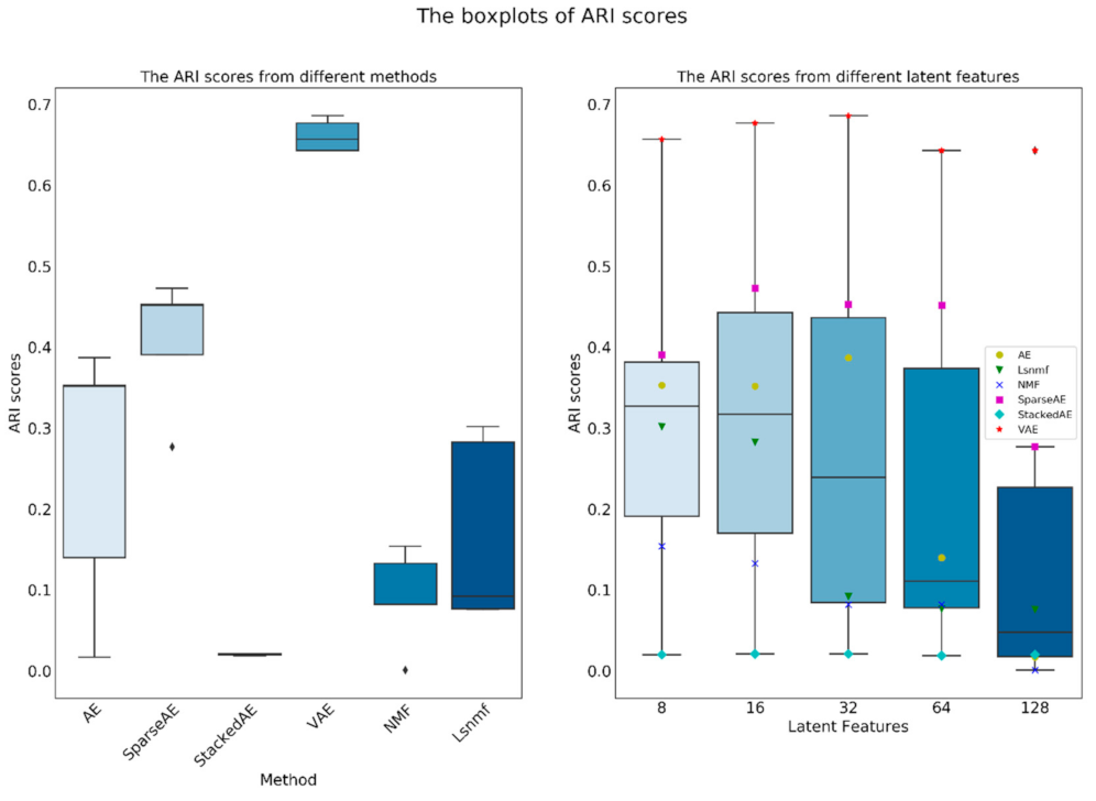
Since the number of latent features can be set manually, we made an additional work which used 8, 16, 32, 64 and 128 latent features as a hyper parameter of the methods. The results were listed in the Supplementary Materials (totaling 30 figures and 6 tables). Using the external results, we made an additional statistic using box plots. Since the distribution of ARI, F1 and NMI scores are similar, only the ARI and Silhouette scores were used in this section (Figure 10 and Figure 11), and the other two figures were listed in the Supplementary Materials (Figures S31 and S32). As shown in Figure 10, VAE significantly outperformed other methods in ARI since the median and the whiskers were higher than other methods. In the rest of the methods, SparseAE showed a relatively better performance in the median and upper whisker. The results in Figure 10 correspond with the results in Section 4.1 that VAE and SparseAE rank as the top two of all the methods. However, the distribution of Silhouette scores was quite different with ARI scores; the NMF achieved the highest score and VAE had the relatively lower distribution among the six methods. This result shown that the NMF is a potential method for information extraction and can separate the hidden information in variant shapes. However, the unsupervised separated clusters from NMF were not the expectation of this work, thus additional modification of the algorithm of NMF seems necessary for characterizing scATAC-seq data.
Regarding the number of latent features (the right side of Figure 10), the evaluation metrics, except Silhouette score, become better when the number of latent features range from around 8 to 32. When the number of latent features becomes larger than 32, the overall performance reduced gradually. Therefore, using 10 and 20 latent features in this work is appropriate. Generally, when using manifold learning methods for information extracting, usually the number of latent features is not linearly corrected with the final performance because the extractable information contained by the data is limited, and the performance will reduce after the number of latent features exceed a certain threshold. In this work, considering the scores of both VAE and SparseAE were increasing from 8 to 16 latent features, we think the threshold is near 16–32, but the specific value will be changed according to the used method.
4.3. The Separation of EX Cells
As demonstrated in Section 3.7, even using VAE, the globally outperformed method in this work, the EX cells were not as well separated as other cells. However, according to Figure 6, the mis-separation usually occurred only in EX cells, which means VAE is able to separate the EX cells and non-EX cells, but will mix the subtype of EX1, EX2 and EX3 cells. Considering the algorithm of VAE, the mis-separation of the EX cells has shown that the Gaussian distribution generated by the encoders of the EX cells are similar, or more similar than with other non-EX cells so that K-means cannot tell the different subtypes as well as others. As evidence, the UMAP in Figure 6 showed that the cells of EX1, EX2 and EX3 were so close to each other and relatively far away from other cells. Since UMAP is only a projection of the high -dimensional data from the latent variable, we think using an unsupervised method to separate the EX cells is a new challenge for us to solve in the future.
5. Conclusions
In summary, this work provided multiple symmetric autoencoder architecture and NMF methods for characterizing scATAC-seq data. If similar data were used, VAE and SparseAE could be good candidates for dimension reduction and feature extraction. At present, all types of cells except EX can be well separated. It is meaningful to suggest a more in-depth study of VAE or to look for more effective methods to better separate subtypes of EX in the future. These results would be helpful for the related research which needs a selection strategy of high-dimensional and extremely sparse data processing.
Supplementary Materials
The following figures and tables recording the results of the additional work which used 8, 16, 32, 64 and 128 latent features of the six characterizing methods and the additional statistic figures mentioned in Section 4.2 are available online at https://0-www-mdpi-com.brum.beds.ac.uk/article/10.3390/sym13081467/s1.
Author Contributions
Conceptualization, Y.H. and R.J.; methodology, Y.H.; software, Y.H.; validation, Y.H., Y.L. (Yizhou Li) and Y.L. (Yuan Liu); formal analysis, Y.H.; investigation, Y.H.; resources, Y.H.; data curation, Y.H.; writing—original draft preparation, Y.H.; writing—review and editing, R.J.; visualization, Y.H.; supervision, M.L. and R.J.; project administration, M.L.; funding acquisition, M.L. All authors have read and agreed to the published version of the manuscript.
Funding
This research was funded by the National Natural Science Foundation of China, grant number 21775107.
Institutional Review Board Statement
Not applicable.
Informed Consent Statement
Not applicable.
Data Availability Statement
Not applicable.
Acknowledgments
This work was supported by the grants from the National Natural Science Foundation of China, China (no. 21775107).
Conflicts of Interest
The authors declare no conflict of interest.
Abbreviations
The following abbreviations are used in this manuscript:
| SparseAE | Sparse autoencoder |
| StackedAE | Stacked autoencoder |
| VAE | Variational autoencoder |
| NMF | Nonnegative Matrix Factorization |
| Lsnmf | Alternating Nonnegative Least Squares Matrix Factorization |
| ARI | Adjusted Rand Index |
| NMI | Normalized mutual information |
| UMAP | Uniform Manifold Approximation and Projection |
References
- Buenrostro, J.D.; Giresi, P.G.; Zaba, L.C.; Chang, H.Y.; Greenleaf, W.J. Transposition of native chromatin for fast and sensitive epigenomic profiling of open chromatin, DNA-binding proteins and nucleosome position. Nat. Methods 2013, 10, 1213–1218. [Google Scholar] [CrossRef]
- Buenrostro, J.D.; Wu, B.; Litzenburger, U.M.; Ruff, D.; Gonzales, M.L.; Snyder, M.P.; Chang, H.Y.; Greenleaf, W.J. Single-cell chromatin accessibility reveals principles of regulatory variation. Nature 2015, 523, 486–490. [Google Scholar] [CrossRef] [PubMed]
- Cusanovich, D.A.; Daza, R.; Adey, A.; Pliner, H.A.; Christiansen, L.; Gunderson, K.L.; Steemers, F.J.; Trapnell, C.; Shendure, J. Multiplex single-cell profiling of chromatin accessibility by combinatorial cellular indexing. Science 2015, 348, 910–914. [Google Scholar] [CrossRef] [PubMed] [Green Version]
- Granja, J.M.; Corces, M.R.; Pierce, S.E.; Bagdatli, S.T.; Choudhry, H.; Chang, H.Y.; Greenleaf, W.J. ArchR is a scalable software package for integrative single-cell chromatin accessibility analysis. Nat. Genet. 2021, 53, 403–411. [Google Scholar] [CrossRef] [PubMed]
- Stuart, T.; Butler, A.; Hoffman, P.; Hafemeister, C.; Satija, R. Comprehensive Integration of Single-Cell Data. Cell 2019, 177, 1888–1902. [Google Scholar] [CrossRef]
- Wolf, F.A.; Angerer, P.; Theis, F.J. SCANPY: Large-scale single-cell gene expression data analysis. Genome Biol. 2018, 19, 15. [Google Scholar] [CrossRef] [PubMed] [Green Version]
- Trapnell, C.; Cacchiarelli, D.; Grimsby, J.; Pokharel, P.; Li, S.; Morse, M.; Lennon, N.J.; Livak, K.J.; Mikkelsen, T.S.; Rinn, J.L. The dynamics and regulators of cell fate decisions are revealed by pseudotemporal ordering of single cells. Nat. Biotechnol. 2014, 32, 381–386. [Google Scholar] [CrossRef] [Green Version]
- Fang, R.; Preissl, S.; Hou, X.; Lucero, J.; Ren, B. Fast and Accurate Clustering of Single Cell Epigenomes Reveals Cis-Regulatory Elements in Rare Cell Types. bioRxiv 2019. [Google Scholar] [CrossRef] [Green Version]
- Murtuza, B.S.; Connor, R.; Andrew, H.; Sharrocks, A.D.; Magnus, R. Classifying cells with Scasat, a single-cell ATAC-seq analysis tool. Nuclc Acids Res. 2019, 47, e10. [Google Scholar]
- González-Blas, C.B.; Minnoye, L.; Papasokrati, D.; Aibar, S.; Hulselmans, G.; Christiaens, V.; Davie, K.; Wouters, J.; Aerts, S. cisTopic: Cis-regulatory topic modeling on single-cell ATAC-seq data. Nat. Methods 2019, 16, 397–400. [Google Scholar] [CrossRef]
- Mahdi, Z.; Lin, Z.; Timothy, D.; Chen, X.; Zhana, D.; Alicia, S.; Greenleaf, W.J.; Hung, W.W. Unsupervised clustering and epigenetic classification of single cells. Nat. Commun. 2018, 9, 2410. [Google Scholar]
- Yu, W.; Uzun, Y.; Zhu, Q.; Chen, C.; Tan, K. ScATAC-pro: A comprehensive workbench for single-cell chromatin accessibility sequencing data. Genome Biol. 2020, 21, 94. [Google Scholar] [CrossRef] [Green Version]
- Kingma, D.P.; Welling, M. Auto-Encoding Variational Bayes. arXiv 2014, arXiv:1312.6114. [Google Scholar]
- Lopez, R.; Regier, J.; Cole, M.B.; Jordan, M.I.; Yosef, N. Deep generative modeling for single-cell transcriptomics. Nat. Methods 2018, 15, 1053–1058. [Google Scholar] [CrossRef]
- Xiong, L.; Xu, K.; Tian, K.; Shao, Y.; Tang, L.; Gao, G.; Zhang, M.; Jiang, T.; Zhang, Q.C. SCALE method for single-cell ATAC-seq analysis via latent feature extraction. Nat. Commun. 2019, 10, 4576. [Google Scholar] [CrossRef]
- Grnbech, C.H.; Vording, M.F.; Timshel, P.; Snderby, C.K.; Winther, O. scVAE: Variational auto-encoders for single-cell gene expression data. Bioinformatics 2020, 36, 4415–4422. [Google Scholar] [CrossRef]
- Cao, Y.; Fu, L.; Wu, J.; Peng, Q.; Xie, X. SAILER: Scalable and Accurate Invariant Representation Learning for Single-Cell ATAC-Seq Processing and Integration. bioRxiv 2021. [Google Scholar] [CrossRef]
- Kramer, M.A. Nonlinear principal component analysis using autoassociative neural networks. AIChE J. 1991, 37, 233–243. [Google Scholar] [CrossRef]
- Goodfellow, I.; Bengio, Y.; Courville, A. Deep Learning; MIT Press: Cambridge, MA, USA, 2016. [Google Scholar]
- Makhzani, A.; Frey, B. k-Sparse Autoencoders. arXiv 2013, arXiv:1312.5663. [Google Scholar]
- Ng, A. Sparse autoencoder. CS294A Lect. Notes 2011, 72, 1–19. [Google Scholar]
- Bengio, Y.; Lecun, Y. Scaling Learning Algorithms Towards AI. In Large-Scale Kernel, Machines; Bottou, L., Chapelle, O., DeCoste, D., Weston, J., Eds.; MIT Press: Cambridge, UK, 2007. [Google Scholar]
- Shao, C.; Höfer, T. Robust classification of single-cell transcriptome data by nonnegative matrix factorization. Bioinformatics 2017, 33, 235–242. [Google Scholar] [CrossRef] [PubMed]
- Preissl, S.; Fang, R.; Huang, H.; Zhao, Y.; Raviram, R.; Gorkin, D.U.; Zhang, Y.; Sos, B.C.; Afzal, V.; Dickel, D.E. Single-nucleus analysis of accessible chromatin in developing mouse forebrain reveals cell-type-specific transcriptional regulation. Nat. Neurosci. 2018, 21, 432–439. [Google Scholar] [CrossRef] [PubMed] [Green Version]
- Mcinnes, L.; Healy, J. UMAP: Uniform Manifold Approximation and Projection for Dimension Reduction. J. Open Source Softw. 2018, 3, 861. [Google Scholar] [CrossRef]
- Van der Maaten, L.; Hinton, G.E. Visualizing High-Dimensional Data using t-SNE. J. Mach. Learn. Res. 2008, 9, 2579–2605. [Google Scholar]
- Paszke, A.; Gross, S.; Massa, F.; Lerer, A.; Chintala, S. PyTorch: An Imperative Style, High-Performance Deep Learning Library. Adv. Neural Inf. Process. Syst. 2019, 32, 8026–8037. [Google Scholar]
- Kingma, D.; Ba, J. Adam: A Method for Stochastic Optimization. arXiv 2014, arXiv:1412.6980. [Google Scholar]
- Hinton, G.E.; Krizhevsky, A.; Wang, S.D. Transforming Auto-Encoders; Springer: Berlin/Heidelberg, Germany, 2011; pp. 44–51. [Google Scholar]
- Liou, C.Y.; Cheng, W.C.; Liou, J.W.; Liou, D.R. Autoencoder for words. Neurocomputing 2014, 139, 84–96. [Google Scholar] [CrossRef]
- Liu, G.; Bao, H.; Han, B. A Stacked Autoencoder-Based Deep Neural Network for Achieving Gearbox Fault Diagnosis. Math. Probl. Eng. 2018, 2018, 5105709. [Google Scholar] [CrossRef] [Green Version]
- Doersch, C. Tutorial on Variational Autoencoders. arXiv 2016, arXiv:1606.05908. [Google Scholar]
- Goodfellow, I.J.; Pouget-Abadie, J.; Mirza, M.; Xu, B.; Warde-Farley, D.; Ozair, S.; Courville, A.; Bengio, Y. Generative Adversarial Networks. Adv. Neural Inf. Process. Syst. 2014, 3, 2672–2680. [Google Scholar] [CrossRef]
- Dilokthanakul, N.; Mediano, P.; Garnelo, M.; Lee, M.; Salimbeni, H.; Arulkumaran, K.; Shanahan, M. Deep Unsupervised Clustering with Gaussian Mixture Variational Autoencoders. arXiv 2016, arXiv:1611.02648. [Google Scholar]
- Koren, Y.; Bell, R.; Volinsky, C. Matrix factorization techniques for recommender systems. Computer 2009, 42, 30–37. [Google Scholar] [CrossRef]
- Dhillon, I.; Sra, S. Generalized Nonnegative Matrix Approximations with Bregman Divergences. In Neural Information Processing Systems; MIT Press: Vancouver, BC, Canada, 2005; pp. 283–290. [Google Scholar]
- Ren, B.; Pueyo, L.; Chen, C.; Choquet, É.; Debes, J.H.; Duchêne, G.; Ménard, F.; Perrin, M.D. Using Data Imputation for Signal Separation in High Contrast Imaging. Astrophys. J. 2020, 892, 74. [Google Scholar] [CrossRef]
- Ben, M.; Thomas, W.; Jan, B.; Robert, K.; Sasha, M.; Gerdus, B.; Du, B.L.; Daniel, K.; Tristan, H.; Konrad, S. Non-Negative Matrix Factorization for Learning Alignment-Specific Models of Protein Evolution. PLoS ONE 2011, 6, e28898. [Google Scholar]
- Lee, D.D.; Seung, H.S. Learning the parts of objects by non-negative matrix factorization. Nature 1999, 401, 788–791. [Google Scholar] [CrossRef]
- Hoyer, P.O. Nonnegative matrix factorization with sparseness constraints. J. Mach. Learn. Res. 2004, 5, 1457–1469. [Google Scholar]
- Zitnik, M.; Zupan, B. NIMFA: A Python Library for Nonnegative Matrix Factorization. J. Mach. Learn. Res. 2012, 13, 849–853. [Google Scholar]
- Lin, C. Projected Gradient Methods for Nonnegative Matrix Factorization. Neural Comput. 2014, 19, 2756–2779. [Google Scholar] [CrossRef] [Green Version]
- Wang, G.; Kossenkov, A.V.; Ochs, M.F. LS-NMF: A modified non-negative matrix factorization algorithm utilizing uncertainty estimates. BMC Bioinform. 2006, 7, 175. [Google Scholar]
- Arthur, D.; Vassilvitskii, S. k-means++: The advantages of careful seeding. In Proceedings of the Eighteenth Annual ACM-SIAM Symposium on Discrete Algorithms, New Orleans, LA, USA, 7–9 January 2007; pp. 1027–1035. [Google Scholar]
- Hubert, L.; Arabie, P. Comparing partitions. J. Classif. 1985, 2, 193–218. [Google Scholar] [CrossRef]
Figure 1.
Workflow of the whole process. First, four kinds of neural networks and two kinds of matrix factorization were used to reduce dimension (step 1). Then, UMAP was used to embed the latent features to 2 dimensions and K-means clustered on the extracted low dimensional potential variables (i.e., latent features) to obtain cluster assignments (step 2).

Figure 2.
Feature embedding and clustering of autoencoder under different latent space. Clustering accuracy was shown in evaluation matrices between cluster assignments predicted by K-means and the reference cell types. The blue color bar refers to the number of cells; (a,c) UMAP visualization of the extracted features from SparseAE with the different number of latent features; (b,d) evaluation matrices with the different number of latent features.

Figure 3.
Feature embedding and clustering of autoencoder under different number of latent features. Clustering accuracy was shown in evaluation matrices between cluster assignments predicted by K-means and the reference cell types. The blue color bar refers to the number of cells.
Figure 3.
Feature embedding and clustering of autoencoder under different number of latent features. Clustering accuracy was shown in evaluation matrices between cluster assignments predicted by K-means and the reference cell types. The blue color bar refers to the number of cells.

Figure 4.
Feature embedding and clustering of SparseAE under different latent space. Clustering accuracy was shown in evaluation matrices between cluster assignments predicted by K-means and the reference cell types. The blue color bar refers to the number of cells; (a,c) UMAP visualization of the extracted features from SparseAE with the different number of latent features; (b,d) evaluation matrices with the different number of latent features.

Figure 5.
Feature embedding and clustering of StackedAE under different latent space. Clustering accuracy was shown in evaluation matrices between cluster assignments predicted by K-means and the reference cell types. The blue color bar refers to the number of cells; (a,c) UMAP visualization of the extracted features from StackedAE with the different number of latent features; (b,d) evaluation matrices with the different number of latent features.

Figure 6.
Feature embedding and clustering of VAE under different latent space. Clustering accuracy was shown in evaluation matrices between cluster assignments predicted by K-means and the reference cell types. The blue color bar refers to the number of cells; (a,c) UMAP visualization of the extracted features from VAE with the different number of latent features; (b,d) evaluation matrices with the different number of latent features.

Figure 7.
Feature embedding and clustering of NMF under different latent space. Clustering accuracy was shown in evaluation matrices between cluster assignments predicted by K-means and the reference cell types. The blue color bar refers to the number of cells; (a,c) UMAP visualization of the extracted features from NMF with the different number of latent features; (b,d) evaluation matrices with the different number of latent features.

Figure 8.
Feature embedding and clustering of Lsnmf under different latent space. Clustering accuracy was shown in evaluation matrices between cluster assignments predicted by K-means and the reference cell types. The blue color bar refers to the number of cells; (a,c) UMAP visualization of the extracted features from Lsnmf with the different number of latent features; (b,d) evaluation matrices with the different number of latent features.

Figure 9.
Feature embedding and clustering of VAE and SparseAE of the embedded layer with 10 latent features in case of EX1, EX2 and EX3 are seen as an entire class: EX. Clustering accuracy was shown in evaluation matrices between cluster assignments predicted by k-means and the reference cell types. The blue color bar refers to the number of cells; (a,c) UMAP visualization of the extracted features from VAE and SparseAE; (b,d) evaluation matrices of VAE and SparseAE.

Figure 10.
The boxplots of ARI scores generated from different methods and latent features. In the figure the black Diamond (◊) is outlier.
Figure 10.
The boxplots of ARI scores generated from different methods and latent features. In the figure the black Diamond (◊) is outlier.

Figure 11.
The boxplots of Silhouette scores generated from different methods and latent features. In the figure, few marker were overlapped. For example, the marker ‘Җ’ in blue is the NMF on the upper whisker, and the black Diamond (◊) is outlier.
Figure 11.
The boxplots of Silhouette scores generated from different methods and latent features. In the figure, few marker were overlapped. For example, the marker ‘Җ’ in blue is the NMF on the upper whisker, and the black Diamond (◊) is outlier.


Table 1.
Brief introduction of autoencoders structure.
| Auto-Encoders | Encoder Layer | Encoder 1 | Decoder Layer | Decoder 1 | Optimizer |
|---|---|---|---|---|---|
| General autoencoder | (1024-128) | ReLU | Nan 2 | Sigmoid | Adam |
| Sparse autoencoder | (30) | ReLU | Nan 2 | Sigmoid | Adam |
| Stacked autoencoder | (8192-2048-256) | ReLU | (256-2048-8192) | ReLU | SGD |
| Variational autoencoder | (1024-128) | ReLU | Nan 2 | Sigmoid | Adam |
1 activation function. 2 directly connects the output layer.
Table 2.
The clustering performance using the methods with different dimension of latent features.
| Methods | Latent Feature Number | F1 Score | ARI | NMI | Silhouette_Score |
|---|---|---|---|---|---|
| Autoencoder | 10 | 0.54 | 0.342 | 0.464 | 0.198 |
| 20 | 0.54 | 0.341 | 0.481 | 0.188 | |
| SparseAE | 10 | 0.71 | 0.499 | 0.584 | 0.065 |
| 20 | 0.67 | 0.481 | 0.571 | 0.056 | |
| StackedAE | 10 | 0.21 | 0.020 | 0.068 | 0.340 |
| 20 | 0.22 | 0.025 | 0.072 | 0.199 | |
| VAE | 10 | 0.85 | 0.666 | 0.731 | 0.223 |
| 20 | 0.85 | 0.664 | 0.730 | 0.236 | |
| NMF | 10 | 0.45 | 0.158 | 0.364 | 0.339 |
| 20 | 0.36 | 0.082 | 0.255 | 0.298 | |
| Lsnmf | 10 | 0.55 | 0.314 | 0.504 | 0.283 |
| 20 | 0.46 | 0.343 | 0.483 | 0.168 |
Table 3.
The clustering performance using VAE and SparseAE with the embedded layer with 10 latent features in the case of EX1, EX2 and EX3 are seen as an entire class.
Table 3.
The clustering performance using VAE and SparseAE with the embedded layer with 10 latent features in the case of EX1, EX2 and EX3 are seen as an entire class.
| Methods | F1 Score | ARI | NMI | Silhouette_Score |
|---|---|---|---|---|
| VAE | 0.94 | 0.902 | 0.828 | 0.259 |
| SparseAE | 0.82 | 0.767 | 0.670 | 0.065 |
Publisher’s Note: MDPI stays neutral with regard to jurisdictional claims in published maps and institutional affiliations. |
© 2021 by the authors. Licensee MDPI, Basel, Switzerland. This article is an open access article distributed under the terms and conditions of the Creative Commons Attribution (CC BY) license (https://creativecommons.org/licenses/by/4.0/).
Share and Cite
MDPI and ACS Style
Huang, Y.; Li, Y.; Liu, Y.; Jing, R.; Li, M. A Multiple Comprehensive Analysis of scATAC-seq Based on Auto-Encoder and Matrix Decomposition. Symmetry 2021, 13, 1467. https://0-doi-org.brum.beds.ac.uk/10.3390/sym13081467
AMA Style
Huang Y, Li Y, Liu Y, Jing R, Li M. A Multiple Comprehensive Analysis of scATAC-seq Based on Auto-Encoder and Matrix Decomposition. Symmetry. 2021; 13(8):1467. https://0-doi-org.brum.beds.ac.uk/10.3390/sym13081467
Chicago/Turabian StyleHuang, Yuyao, Yizhou Li, Yuan Liu, Runyu Jing, and Menglong Li. 2021. "A Multiple Comprehensive Analysis of scATAC-seq Based on Auto-Encoder and Matrix Decomposition" Symmetry 13, no. 8: 1467. https://0-doi-org.brum.beds.ac.uk/10.3390/sym13081467
Note that from the first issue of 2016, this journal uses article numbers instead of page numbers. See further details here.