Article

Quantification of Sub-Solar Star Ages from the Symmetry of Conjugate Histograms of Spin Period and Angular Velocity

by
Robert E. Criss
and
Anne M. Hofmeister
*
Department of Earth and Planetary Science, Washington University, St Louis, MO 63130, USA
*
Author to whom correspondence should be addressed.
Submission received: 12 June 2021 / Revised: 2 August 2021 / Accepted: 3 August 2021 / Published: 18 August 2021
(This article belongs to the Special Issue Astronomy and Symmetry)

Abstract

:
Empirical laws proposed for the decline in star spin with time have heretofore been tested using ambiguous fitting models. We develop an analytical inverse model that uses histogram data to unequivocally determine the physical law governing how dwarf star spin depends on time (t) and mass (M). We analyze shapes of paired histograms of axial rotation period (П) and angular velocity (ω = 2π/П) to utilize the fact that a variable and its reciprocal are governed by the same physics. Copious data on open clusters are used to test the formula ∂ω/∂t ∝ − ωn where n is unrestricted, and thus covers diverse possibilities. Histogram conjugates for each of 15 clusters with 120 to 812 measurements provide n = 1.13 ± 0.19. Results are independent of initial spin rate, bin size, cluster parameters, and star mass. Notably, 11 large clusters with mostly M-types yield fits with n = 1.07 ± 0.12. Associations behave similarly. Only exponential decay (n = 1) explains the similar shapes of the conjugate histograms for the spin period and angular velocity, despite the asymmetric (inverse) relationship of these variables. This rate law is consistent with viscous dissipation. Forward modeling confirms that n is near unity and further shows that coeval formation of all stars in a cluster does not occur. We therefore explore a constant rate of star production, which is reasonable for tiny stars. Inverse models show that episodic production increases with mass, but is unimportant below ~0.55 MSun. We infer star and cluster ages, and find that star production becomes less regular with time, as interstellar gas and dust are progressively depleted. Our new analytical approach of extracting a physical law from conjugate histograms is general and widely applicable.

1. Introduction

Star ages are very important to astronomy as they are intimately linked to stellar processes and evolution (e.g., [1,2,3]). Of all the stars, only our Sun has a known age, which is based on consistency among isotopic data for diverse meteorite types [4]. Ages of other stars are inferred from various models of stellar evolution where cluster ages are sometimes incorporated, but these too are derived from models.
One ubiquitous and measurable indicator of a star’s age is its axial spin rate, which declines with time: young stars have periods (П) as short as a few hours [5,6], whereas our ancient, 4.54 Ga (4.54 × 10⁹ year-old) Sun spins slowly with П ~ 24.5 d at its equator. Different rate laws for spin decay with time have been proposed [7,8], but have not been validated [9]. The currently popular approach of gyrochronology is detailed below along with its known problems [10,11].
Given the lack of isotopic data on star ages, a statistical test of spin decay models is appropriate. Robust tests are possible because the database on spin rates now includes 11 open clusters that each have period measurements for >243 stars, plus several clusters and associations with at least 120 measurements (Table 1). Statistics were once used to study stellar rotation [12], but this approach was abandoned, in part because the methods used to measure spin rates have changed. Prior to ~1996, Doppler methods provided apparent tangential velocities (vsini) of rotating stars. Converting these data to rotation periods (П) requires estimating both stellar radius (R) and orientation (i) of the spin axis, because П = 2πR/vequator. Moreover, period is undefined (not measureable) at an inclination of 0°.
Current methods ascertain spin periods by tracking luminosity variations (light curves), and thereby avoid the ambiguity associated with star orientation and size. The database has recently exploded due to Kepler Mission searches for exoplanets and extraterrestrial life, which have focused on very small dwarf stars (red M-types and orange K-types: Table 1). These star types dominate cluster populations (Figure 1a).
Recent studies furthermore characterize the stars by a color index, with reference to various filters. Frequently, the B-V filter is used (Table 1). Color index is important because, except for spin period, it links to all major star properties: surface temperature, luminescence, radius, and mass (M), through simple proportionalities (e.g., [37,38]; Figure 1b). Thus, starspot studies provide both angular velocities (ω) and equatorial tangential velocity via:
ω = 2π/П = v/R
Given the interconnected physical properties, the interrelationships of star spin, age, and mass are of great interest.

1.1. Purpose

We use a new tactic to establish the rate law for spin-down, which is to examine conjugate pairs of histograms of the same data. Our inverse method (Section 3) is mathematically novel but straightforward, and makes very few assumptions. Examining both П- and ω-histograms is essential because histograms of angular velocity place emphasis on old stars whereas histograms of period emphasize young stars. We also develop a new method to analyze histograms that are incomplete or under-sampled, and utilize forward modeling to test assumptions.

1.2. Organization

Section 2 provides background information on analytical inverse models because this approach is uncommon. Section 2 also summarizes the existing database on star spin, and the currently popular methodologies. Section 3 presents our analytical mathematics. Section 3.1 constructs histograms for the endmember case of coeval production and of stars forming with random initial spin rates, to evaluate the feasibility of these popular scenarios. Section 3.2 develops our basic model. Section 3.3 and Section 3.4 show that assuming steady-state production of stars with time has a minor effect in our approach. Section 3.5 develops a new method for removing possible effects of bin size in histogram analysis. Section 4 demonstrates that exponential decay best represents star spin data and that other proposed rates of decay are inconsistent with observed histogram shapes. Section 5 evaluates whether possible mechanisms are consistent with exponential spin loss. Section 6 calibrates our formula for the dependence of spin rate (or period) on stellar age and M/MSun, using the age of the Sun and some limiting values.
Astronomical implications of exponential spin-down for main sequence dwarfs are covered in Section 7. This concluding section also addresses wide applicability of our analytical inverse methods to statistical data bases that can be represented as histograms.

2. Background

2.1. Inverse vs. Forward Modeling

A mainstay of modern science is using forward models with many parameters to explain data. Fitting has utility in that measurements can be reproduced and trends extrapolated, but the drawback is that an incorrect physical model can appear to match data via trade-offs among unconstrained input parameters, particularly when multiplied [46]. In contrast, analytical inverse models provide unique solutions [47,48]. Many analytical inverse approaches are historic. Groetsch [47] provides diverse examples from many fields. The astronomical example most closely related to the goals and approach of the present paper is the extraction of the proper motions of stars from observed radial velocities [49]. Recently, an inverse approach was used to extract mass and density of spiral galaxies from measurements of their rotational velocities as a function of radius [50].

2.2. Useful Mathematical Attributes of Histograms

Histograms are commonly used to visualize data. A histogram is described by a density function that has a corresponding distribution function that embodies the underlying physics [51]. Histograms of a variable and of its reciprocal typically have different shapes because their density functions differ in mathematical form, yet the underlying physical law is the same. On this basis, we develop an inverse method to extract a physical law from histogram shapes. Our approach assumes that one independent variable largely controls the dependent variable embodied by any given histogram. Consequently, the reciprocated dependent variable and its histogram are also controlled by the same independent variable. Our method is general, but as is common with inverse modeling, the mathematical model is deduced through solving a specific problem [47].

2.3. The Database on Spin Periods of Dwarf Stars

Star periods from analyzing light curves (intensity vs. time) are independent of the axial orientation of the star. Data quality is covered in many publications on light curves of cluster stars. Issues such as biases, measures of completeness, and minimal contamination from stars outside the cluster are addressed in detail by Hartman et al. [27]. Briefer discussions exist in Irwin et al. [16,19,25], and in most studies since 2015.
Importantly, spin values do not depend strongly on the research group: c.f. Irwin et al. [25] to Jackson and Jeffries [52]. An example is the Hyades, where 90% of the stars examined in more than one study have periods that match to better than 10% [53]. For Praesepe, periods for half of the 214 stars measured multiple times agree within 2%, and ¾ of the repeats agree within 5% [29]. Thus, the available data should be accurate to better than 10%, with some outliers. Differences among studies prior to 2018 due to methodology seem moot. Notably, more recent studies use a different approach. Statistically, period measurements are no different, as shown by Cui et al. [54] via comparison with 1107 stars measured by McQuillen et al. [55]: the majority of periods agree within 1%. However, mass and luminosity are determined in a different manner in the most recent studies, and so these were not used to ascertain the effect of mass, unless mass of the stars was included in the tabulated data. Typically, temperatures were listed.
A few star spot studies of clusters were not analyzed because they either cover the same cluster with a similar mass range (cf. [14] to [56]) and provide very similar histograms, or fewer than 100 stars were measured (e.g., [57,58]). Neither are histograms of aggregated data from Kepler missions presented because, unlike open clusters, star production began at assorted times, which renders extraction of a rate law uncertain.
Importantly, two systematic errors exist in star spot studies.
  • An upper limit on П (and a corresponding lower limit on ω) exists and varies among the studies because starspot lifetimes must exceed the observational duration (e.g., [59]). Hence, stars with periods >25 days are difficult to measure and therefore underrepresented in data from the Kepler campaigns. The reliability study of 38 G-types in M67 found that 75% of the measurements of slow rotations were reliable, but only for П < 32 days [60].
  • For all studies, a lower limit on П (and an upper limit on ω) is affected by factors such as the time between formation and the time at which a detectable (luminous) star exists. Under-representation of slow- and fast-spinning stars is accounted for in our approach (Section 3).
In summary, Section 4 focuses on post-2008 datasets from the Kepler 2 mission on individual open clusters, which are purported to be more accurate and sample more stars. Most studies yield >243 period measurements on individual open clusters, and describe properties of the open cluster studied (Table 1); also see Finlay [61]. Star spot studies of various groupings of stars near the Sun, associations, field M stars, and ground-based measurements are also analyzed. The reference dataset of Mt. Wilson stars includes sufficient information to convert tangential velocity to periods [36].
Data sets were downloaded from published supplementary material associated with the cited papers. Very few datasets were tabulated in the papers.

2.4. Relationships of Mass and Color Needed to Compare Star Spin Studies

This study mostly considers individual clusters. Towards the end of the report, data from the clusters listed in Table 1 are merged to explore of the effect of mass on spin-down. To merge data, we use M/MSun rather than color-temperature because some studies used filters other than B-V. Uncertainties in mass were estimated as ~8% by Hartman et al. [20]. Moreover, the precise manner in which M/MSun is computed is not important to our study because mass is only used to separate the stars into broad categories (e.g., M-types vs. K-types).
Reported mass is used, if available. If not, we used results from Zombeck [38] to construct the following empirical formulae for average mass:
M/MSun ≅ 1.006(B-V + 0.35) − 0.974 [for B-V < 1.15] and M/MSun ≅ 1.808 − 0.9627(B-V) [for B-V > 1.15]
M/MSun ≅ 1.099−0.8058(R-I) + 0.1656(R-I)2,
where R-I is a color index differing from B-V. Using Equation (2) or (3) yielded the same histograms as using the authors’ M/MSun values. Tabulated data for the V-KS index [37] were fit via splining to best cover the wide type ranges of the Pleiades and NCG 2516.

2.5. Formulae Previously Applied to Period Data

The currently popular approach, known as gyrochronology, stems from Skumanich’s [7] proposal that equatorial rotational velocity (v) degrades in proportion to t −1/2, where t is star age. The basis was Ca II emission strengths decreasing as rotational velocities decrease [62], plus model ages for the Pleiades and Hyades star clusters. Stars more massive than the Sun were used in the 1972 proposal, which remains a concern because large stars have very short lifetimes [1] and their properties, including chemical composition, are unlike those of the Sun (Figure 1b) and other dwarf stars. Furthermore, angular momentum losses from our Sun measured from 1994–2019 are a factor of two lower than expected from gyrochronology models [10].
Clearly problems exist with t −1/2 decline, yet alternatives such as exponential decay with time, proposed by Terndrup et al. [8], are little explored. This section therefore focuses on recent modifications of Skumanich’s 1972 idea.
Figure 2a illustrates application of gyrochronology forward modeling to the well-studied Pleiades. Table 2 lists model assumptions of gyrochronology. In summary, data on plots of period vs. B-V are roughly bracketed by two ad hoc curves referred to as the I- and C-trends. The I-trend is alleged to represent slowly rotating stars. The original formula [63]:
П = t ½ [(B-V − 0.5)½ − 0.15(B-V − 0.5)].
was subsequently modified to:
П = 0.7725 t 0.5189 (B-V − 0.4)0.601
[64]. Other empirical relationships with a few free parameters are similar [65]. The narrow range in exponents for time of ½ to 0.57 in current use (e.g., [66]) makes little difference (Figure 2a). Importantly, the square root shape for the I-trend in Figure 2a refers to the ad hoc B-V proportionality of Equation (4), rather than to any dependence on time.
The “C-trend” was proposed [64] to describe fast-spinning stars:
Π = 0.2 exp 0.01 t B-V + 0.1 t 3000 3
This equation is also ad hoc, but is uncommonly used to ascertain age.
Problems in applying the gyrochronology model are recognized [67]. Concerns are as follows:
  • Equations (4)–(6) are fit to only a selected subset of the data, so data on many stars are ignored. From Figure 2, the strong curvature of the I-trend towards low B-V (large mass) differs among the various studies. Thus, the I-trend depends on the particular stars sampled. The axes of Figure 2 do not depict time, and so Skumanich’s proposal of t½ cannot be evaluated from such scatter plots.
  • The C-trend also depends on the particular characteristics of the stars which were sampled (Figure 2a), but the histograms do not, if a sufficient number of stars were measured (Figure 3).
  • A mechanism for catastrophic (coeval) production of all stars in a cluster has not been explained. Counterevidence exists (e.g., [68,69]).
  • Evidence also exists that young stars start with spin that is fast (e.g., [5,6]), rather than from random rates.
  • Magnetic braking models fail to reproduce the distributions of Figure 2a when gyrochronology ages are utilized (e.g., [70]), even though this rate law purportedly describes this loss mechanism.
Four additional problems exist, but have not been discussed in the literature:
  • The postulated trends for fast and slow rotators cross near solar mass (Figure 2a) for which B-V = 0.61 [37], showing gyrochronology models unrealistically require G2 stars to occupy a very narrow range of periods, and provide impossible, imaginary periods for more massive stars.
  • Gyrochronology calculations for 0.3MSun (Equations (5) and (6)) based on model cluster ages only describe data on NGC 2516 (Figure 2b). No solar mass stars in any of the clusters of Table 1 agree with this empirical formulation (Figure 2c).
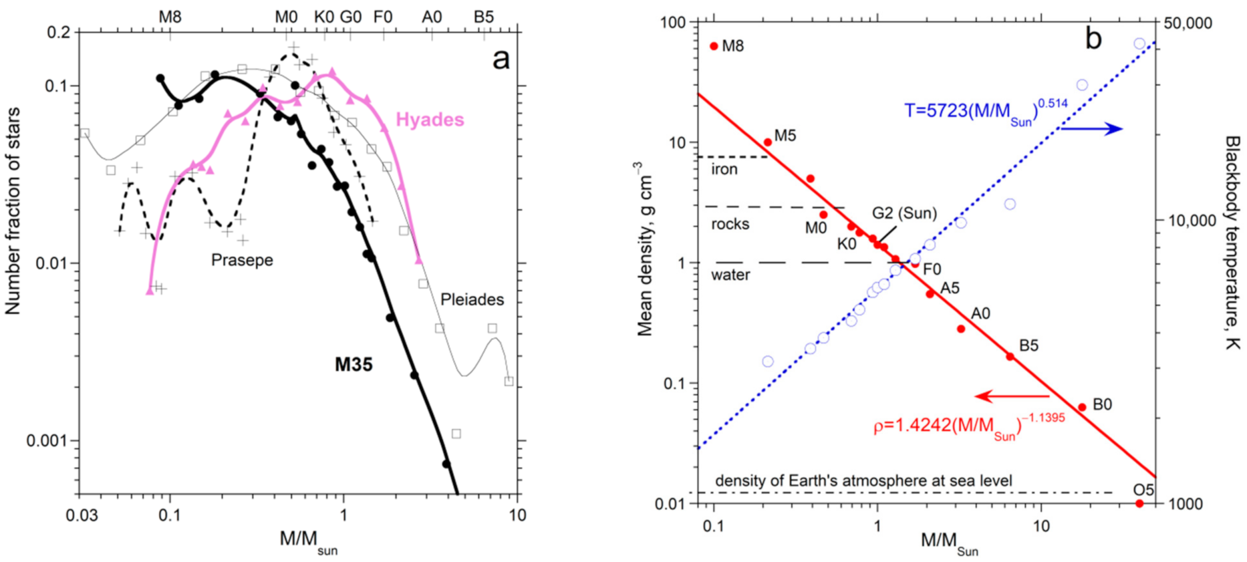
  • The I-trend reflects two factors other than aging of the star: namely, that Kepler missions have a maximum reliable period, and that M-type stars are volumetrically much more abundant than more massive stars (Figure 1a) and so statistically are likely to reveal a broader range of periods plus this upper limit.
  • Equations (4)–(6) require peculiar dimensions for their numerical constants, which results from color-period diagrams not depicting elapsed time.
To address known problems with gyrochronology models, recent studies propose more complicated multi-parameter models and “trends” in addition to C- and I-proposals (e.g., [11]). The age for our Sun is utilized, whereas other ages are gleaned from models. However, adding more equations and more parameters does not remedy the above flaws in gyrochronology, exemplified in Figure 2. These plots show that the slowest rotators detected depend on the maximum period that can be measured in finite duration missions (~25 days), whereas the fastest rotators detected (generally 0.1 to 0.5 days) depend on resolving periodicity from noise in the signal. Thus, the C- and I-trends largely reflect limitations of the measurements, not behavior of stars.
The remainder of our paper focuses on extracting a mass and time dependence from the measurements using an inverse approach. Skumanich’s simple proposal for the time-dependence of spin decay, which differs from the problematic gyrochronology formulations (Figure 2), is evaluated below.

3. Quantitative, Mathematical Analysis of Star Spin Histograms

Loss of spin of rotating stars with time is described by the general formula:
ω t = α ω n
where the exponent n can be non-integer. The proportionality constant α has units that depend on n. For the case of exponential decay (n = 1), τ = 1/α is the mean lifetime. If n = 0, then spin loss is controlled by factors other than spin, whereas n = 3 corresponds to Skumanich’s “rule”.
Solutions to Equation (7) are:
ω = ω 0 e α t   and   Π = Π 0 e + α t   [ for   n = 1 ]
ω1−n = ω01−n + (n−1)αt and Пn−1 = П0n−1 +(2π)n−1(n−1)αt [for n ≠ 1]
As in all previous studies, we assume that a star of a given mass starts its ignited life with a certain initial spin rate (ω0) corresponding to a certain period (П0) and then slows down with time. Below, we use available data to decipher the best value of n, for each of many clusters, that controls the rate at which spin is lost on average, and then evaluate possible effects of stellar mass on the rate law. Consistency of the results is used to establish the physical law governing spin-down.

3.1. Histogram Shapes Do Not Support Coeval Star Production with Random Initial Spins

This section analytically tests a key assumption underlying previous models for star spin-down (Table 2), namely that of simultaneous star formation in any given cluster. To probe the initial conditions, both ω and ω0 must be considered as variables. Equations (8) and (9) lead to:
ω ω 0 = ω ω 0 n
Let us define a parameter G in terms of the entire histogram with a large number Ntotal of stars: i.e., G = Ntotal × bin width/range of ω0. Assuming random ω0 and defining N as the number of stars in any one bin gives a relationship for incremental changes: Nδω = Gδω0. Rearranging and changing the increment to a derivative and then inserting Equation (10) gives:
N = ω 0 ω G = G ω 0 ω n
For constant G, differentiating Equation (11) and using Equation (10) provides:
N ω = n G ω ω 0 ω 2 n 1 ω 0 ω n
The quantity in square brackets is zero for n = 1, positive for n > 1, and negative for n < 1. The slope ∂N/∂ω is thus zero for the exponential form, whereas slopes are positive for n > 1 and n < 0, but negative for 0 < n < 1.
Figure 4 shows numerically generated synthetic histograms that represent coeval star production. First, at t = 0, random initial angular velocities are assumed to exist from 0 up to some limit (ω0 = 0 to 1 in arbitrary units). How this synthetic cluster would appear at two finite times is illustrated for two cases: n = 1 (exponential decay) and n = 3 (Skumanich’s proposal). The trends in the numerically generated histograms are fully consistent with Equations (11) and (12), confirming that these relationships are correct.
The synthetic shapes computed at finite times by assuming coeval production of stars with random initial spins (Figure 4) are unlike histograms of real data (Figure 3 and Figure 5). The synthetic histogram for n = 3 has a positive slope, which is completely at odds with the strong negative slopes observed for all large clusters that we examined (Figure 3 and Figure 5). Figure 5 represents datasets with more than 243 stars. Similarly, the synthetic histogram for n = 1 has a null slope at all times (Figure 4), so that clusters of all ages should have “boxcar” histograms if production were coeval, which is likewise unsupported. Clearly, all cluster stars are not produced at the same time; the differences between the data in Figure 3 (or Figure 5) and Figure 4 are so extreme that no statistical test is needed. Therefore, we begin by assuming steady-state production rate as an endmember case, because this is the simplest remaining possibility. Section 3.2 and Section 3.3 discuss the effect of relaxing this assumption on the rate law determined from the data.
Figure 4, coupled with (12), demonstrates theoretically that the general shape of the histogram does not change with time if, and only if, decay is exponential. That similar histogram shapes are found for clusters of various presumed ages (Figure 3 and Figure 5) points to exponential decay controlling spin-down, in agreement with the general discussion of Apostol [51]. This finding is irrespective of the details of fitting (Section 3.5 and Section 4) and also of assuming steady-state star-production, which permits an analytical approach (Section 3.3).

3.2. Analytical Approach to Deciphering the Rate Law for Constant Production

To derive the number of spins in a counting bin, we begin with the general rate law of Equation (7). Recasting the general solution for ω and for n ≠ 1 gives:
t = ω 1 n ω 0 1 n α ( n 1 )
Any bin on the histogram is bounded by two frequencies, ωa and ωb, and described by:
t a = ω a 1 n ω 0 1 n α ( n 1 )   and   t b = ω b 1 n ω 0 1 n α ( n 1 )
For several reasons, we assume a constant rate (γ) of production for the stars, i.e., a constant rate at which stars become ignited and their periods can be measured. (1) This assumption provides the philosophical alternative to episodic production, akin to the historical viewpoints of Uniformitarianism and Catastrophism; (2) This assumption allows us to provide an analytical formula and to develop a method to quantitatively analyze paired histogram data. (3) Because the consensus view of catastrophic (coeval) production was ruled out above, we posit steady-state production as a feasible alternative. (4) Most of the data is on young clusters (Table 1), for which steady-state production of tiny stars is reasonable. (5) This assumption can be relaxed and others can be considered via numerical analysis in future work, as the database on measured periods expands. Below, episodic production is considered qualitatively.
For constant production, the number of stars included in a given bin is the product of the production rate × the time interval, and thus:
N γ = t a t b = ω a 1 n ω b 1 n α ( n 1 )
The width of the bin is Δω = ωa − ωb. From Equations (14) and (15), combining the constants γ and α to provide a new constant (β = α/γ) provides:
N = ( ω b + Δ ω ) 1 n ω b 1 n β ( n 1 ) = ω b 1 n ( ω b + Δ ω ) 1 n ω b 1 n 1 β ( n 1 ) = ω b 1 n 1 + Δ ω ω b 1 n 1 β ( n 1 )
We now expand the series assuming that that the bin size is small:
N = ω b 1 n 1 + ( 1 n ) Δ ω / ω b 1 β ( n 1 ) = ω b 1 n ( 1 n ) Δ ω ω b β ( n 1 ) = Δ ω β ω b n
Dropping the subscript b provides the remarkably simple solution:
N ω = Δ ω β ω n
Although the above derivation considered n ≠ 1, the same result holds for the special case of n = 1. Specifically, for n = 1,
ω = ω0e−αt, so t = −(1/α)ln(ω/ω0) = [ln(ω0) − ln(ω)]/α.
Utilizing a Taylor series and following the steps described above provides Equation (18).
For periods, the starting point is Пn−1 = П0n−1 + (2π)n−1(n−1)αt for n ≠ 1. Note that the power is (n−1). Solving for t and following the procedure as above leads to:
N Π = 2 π 1 Δ Π β Π n 2
For the special case of n = 1, the procedure described for angular velocity, analogous to (19), is followed, which results in Equation (20).
In summary, if the stars constituting the histogram are produced at a constant rate, then for any power in the generalized rate law (Equation (7)), the number of stars in each bin of width Δω for the ω histogram is given by (18) while the number of stars for each bin of width ΔП for the П-histograms is given by (20). For both formulae, the constant β = α/γ describes the competition of spin loss to star production. For n = 1 only, both N(ω) and N(П) inversely depend on their variables, due to the special properties of exponential functions. Hence, similar shapes will exist in the П- and ω-histograms if and only if n = 1, consistent with the general analysis of Apostol [51]. Section 4 uses Equations (18) and (20) to directly determine n from data on well-studied clusters.
Note that for small ω and small П, the first bins in the histograms are under-populated because the null values for spin cannot exist in real datasets. Additionally, Equation (18) represents the bulk of the data for which ω is large compared to the increment Δω. Therefore, in comparing real data to the ideal curves, we omit the first bin, unless the cluster has a large number of stars, in which case under-population of the first bin is unimportant. For almost all clusters, we compare the data above ~2Δω and ~2ΔП to Equations (18) and (20). Section 4.4 presents an alternative, numerical analysis which avoids potential problems with the variables being smaller than the increments and with an under—populated first bin. Virtually identical results for n are obtained.

3.3. What If Stars Are Produced with Different Spin Values or Decay at Different Rates?

Importantly, Equations (18) and (20), which describe the number of stars having given spins as a function of spin period or angular velocity, do not depend on the initial period П0 or initial angular velocity ω0, even though these are prominent factors in the rate law solutions, Equations (8) and (9). Instead, the only requirement is that the stars are produced at steady state, with a distribution of initial spin values that likewise does not change with time. Therefore, for steady state production, the starting point (i.e., the specific initial spin for any given star) is immaterial to the histogram shape. Our analysis only presumes that once a star has ignited and is spinning, that it slows down according to a certain rate law. The possibility that this rate law may be mass-dependent is considered below.
The exponent n in the rate law (Equation (7)) is revealed by the shape of the histogram curves. It is only the histogram shape that is important to ascertaining n. Neither the interval, decay constant, production rate, nor initial spin rate are particularly influential.
These findings are important for several reasons. First, our analysis is independent of processes possible for very young stars, such as disk formation or star contraction. Likewise, very old stars, which can experience significant mass loss, also have negligible influence. Second, different clusters can be compared together, as long as these are governed by the same rate law. Third, this behavior permits comparison of stars with different starting points; the only requirement is that stars in any given histogram pair are produced at a steady state, and afterward follow the same rate law (Table 2).

3.4. Effect of Episodic Star Production

If stars in a cluster were produced over a narrow time interval and also with a restricted range in period, then the histograms would display a strong peak at some finite value of П (or ω = 2π/П). The range of initial distributions would control the breadth and shape of such a peak. Such behavior, if sufficiently strong, could interfere with ascertaining the rate law. However, only for the two oldest clusters do strong peaks exist (Figure 5k,l). A moderate peak does exist for the old Hyades cluster, but few stars were measured (Figure 6). In all other well-populated histograms (Figure 3 and Figure 5a–j), peaks are weak, if they exist and are associated with the larger stars. This is clearly the case for M34, which also has few data points (Figure 6b). Nevertheless, most fits are compatible with n = 1. For the sub-solar stars emphasized here, the histograms are consistent with nearly constant production, except possibly for the most ancient of clusters. Details are below.

3.5. Bin Size Has a Negligible Effect When Analyzing Paired Histograms

To test whether our choice of bin size affects our results, paired histograms for 4 large clusters with different model ages were fit to a wide range of bin sizes. Large datasets were considered because they permit the test to be conducted over a large range in bin size. The maximum number of bins allowed in our plotting program is 400, which permitted reaching very tiny bin sizes (e.g., 0.1 days). Regarding wide bins, we typically stopped at bin sizes of 5 days or 5 radians per day, which yielded only 10 wide bins (e.g., ~5 day widths). Figure 7 shows very consistent trends in the powers derived from fitting, as in Figure 3, Figure 5 and Figure 6. The average value of n from histogram pairs is always near unity.
As bin size approaches zero, the value of n for the angular velocity histogram decreases whereas the value of n for the period histograms increases. For the power fits shown, n varies from ~0 to ~2. The extracted values of n occupy a narrower range for all bin sizes. When the bin size is small, but not so small as to distort the shapes, n for each histogram type is near unity. Even the old cluster Praesepe, which has a strong peak (Figure 5k), behaves in this manner. Hence, the average n-value for the two fits is used to represent n. The bin size chosen has little effect on the determination of n for the rate law, as demonstrated by the crossover in Figure 7 near 0.2 to 1 widths. Our histograms typically used widths of 0.5 (Figure 3, Figure 5 and Figure 6).

4. Analysis of Histogram Data on Dwarf Star Spin

The primary goal is to determine the integer that best describes the underlying physical law (7). The secondary goal is to ascertain whether the same spin-down law holds for different star types (i.e., different mass ranges). The focus is on open clusters, most of which are active sites of star formation, as indicated by presence of nebulosity, dust, and large, short-lived B-types.

4.1. Individual Clusters

More than 243 stars have been measured in each of 11 clusters (Table 1). The next largest samplings (NGC 2547 and NGC 6811) have 176 and 171 data points, respectively. Figure 5 shows power law fits for the bin count as a function of both ω and П for 12 of these 13 clusters, which are ordered from youngest to oldest in terms of previously modeled cluster ages. Figure 3 shows similarly analyzed Pleiades data, which would place after M50 (Figure 5g). Figure 6 shows two clusters with 120–129 data points. The value of n for each cluster (Table 3) is ascertained by averaging the two fits to ω and П (Equations (8) and (9)).

4.1.1. Fits Are Slightly Affected by Star Mass and Sample Size

The number of measurements weakly affects the fits, showing that statistical significance is obtained for associations with ~200 stars. However, another factor exists: NCG 2547 and NGC 6811 similarly have ~173 data points, but only the former is fit well: the latter, which has only three M-type stars, is fit poorly, due to the presence of a peak in the period distribution (Figure 5l). That this peak is connected with larger stars, rather than with the number of measurements, is supported by comparing M34 to the Hyades (Figure 6), which have 120 and 129 data points, respectively: As above, M34 has a peak, no data on M-types, and does not conform well to a simple power law. Star mass is explored further below.
Notably, the Hyades measurements are highly accurate and yield tightly constrained fits. This finding is consistent with random errors being reduced either as accuracy improves or as sample size increases [71].

4.1.2. Bin Size and Depopulation of Bins near the Origin Have Little Effect

Behavior at short and long ω or П is not important to the analysis. In particular, we found that omitting the first bin does not significantly change the fit (i.e., the variation in n is ~0.1). Figure 7 supports this deduction, since these fits omitted no stars, and further shows that bin size has a negligible effect. Determination of n does not hinge on the values at high and low ω or П, mainly because the result for n depends on the curvature of the histogram. That is, fits mostly depend on bin counts for intermediate values of the variables. Hence, our results depend on the behavior of the majority of the stars, which are those in the “gap” of Figure 2, in contrast to previous work (Section 2.5). In addition, averaging the fits for ω and П to ascertain n reduces the importance of details.

4.1.3. Results of Fitting Individual Clusters

All individual clusters define fits with n near unity, with a range of 0.83 to 1.55. Fits for most clusters yield n between 1.0 and 1.2. The different values of n in the various fits of Figure 3, Figure 5 and Figure 6 are in part connected with zero bin size being impossible to attain. This is more important in fits of the period, since any slow rotators provide small ω. Additionally, applying the inverse relationship of ω with П converts the already broad peaks in П-histograms to very broad and weak peaks in ω-histograms, or adds a peak close to ω = 0, in which region of the histogram also depends on the maximum period measured. For these reasons, angular velocity histograms adhere to power laws more closely than П-histograms. Clearly, investigating pairs of histograms offsets imperfections in the datasets.
Star types of two clusters differ substantially from those of the other 13, but these two still follow exponential decay. Cepheus OB3b (Figure 5c) has some young stars possibly not on the main sequence, and considerable data on comparatively large stars (types F and G-type), see [73] (their Figure 13). Similarly, NGC 869 (Figure 5e) consists of fast (young) rotators and is dominated by type-G stars [15].
Two older clusters with much data (M37 and NGC 2516, Figure 5j,l) plus NGC 6811 with 171 measurements all have n ~ 1.5 (Figure 5k), which is further from unity than values found for younger clusters. Peaks in their distributions cause comparatively poor fits. NGC 681 lacks small M stars. Fitting only the M-types of the other two clusters provides better fits that yield n values closer to unity (Figure 8; Table 3), as is also the case for the Pleiades (Figure 3). Furthermore, peaks in period increase in height with the modeled age of the clusters for the older clusters (Figure 5g–l), whereas young clusters (Figure 5a–f) lack peaks. Middle-aged Pleiades (Figure 3) having a very weak peak is consistent with this finding. Existence of peaks in П, weak or strong, is linked to the presence of old, white dwarfs (Table 3).
The above findings are consistent with star production becoming less regular with time as gas is depleted and mass is stored in white dwarfs, which are not included in period measurements. Notably, peaks in the distribution of M-type stars are only associated with the oldest clusters. These findings show that strong departures from steady-state production affect our fits, but not weak departures. Importantly, n is roughly 1 for all clusters, so for sub-solar dwarfs, star mass does not affect the law for spin decay.
In summary, fits in Figure 3, Figure 5, Figure 6, Figure 7 rule out n < ½ and n > 3/2, and thus unequivocally rule out Skumanich’s rule (n = 3) for MKG stars. Crucially, rate laws with such values for n require that the appearances of the П- and ω-histograms differ substantially (details in Section 3.2), contrary to the copious observations. Exponential decay, proposed by Terndrup et al. [8], best represents the available spin data on dwarf stars in individual clusters. Moreover, production of small stars is continuous in the youngest clusters, but this condition becomes less appropriate for larger stars as the clusters evolve, whereas production of M-types departs from continuous behavior only for the oldest clusters.

4.2. Associations and the Solar Neighborhood

Star associations are less well-bound gravitationally than clusters. The Scorpious-Centaurus OB association [31] includes many young, large B and O stars. Many pre-main sequence stars were sampled: some of which appear to be accreting. Because the sample size (162) is marginally large for a statistical analysis and the data are limited to periods <9 days, the fits are less robust than those discussed above and similar to open clusters with inadequate sampling. Nonetheless, n near 1.1 is inferred (Figure 9a). A larger dataset on similarly young stars (Figure 9b) provides n = 1, within uncertainty. A long period for one star in μ Tau [32] tightly constrains n. The contrasting case of the Solar Neighborhood, which was culled to fast rotators with П < 4 days [33], provides a reasonable fit due to the large number of points (481). This culling removes the old, slow stars and apparently reduces the effect of episodic production.
Thus, two different associations and the Solar Neighborhood behave equivalently to the open clusters, and corroborate that spin decays exponentially with time (Table 3). The period measurements in these recent studies are considered more accurate (e.g., as in the Hyades [28]), which improves reliability of statistical analysis.

4.3. Ground-Based Measurements and a Comparison to Kepler Missions

Ground-based datasets [35,36] are accurate, can include slow rotators, and also provide n near unity (Figure 10). However, the stars sampled need not be related. Thus, observing M-types in the Southern Hemisphere (Figure 10a) provides a generalized sample of the Solar Neighborhood and reveals a peak in П near 100 days, which Kepler missions cannot probe (Figure 9c). This long-period peak is consistent with these M-types being on the order of 4.5 Ga old, like the Sun. Interestingly, the distribution is bimodal, consisting of fast and slow rotating M-types, yet histogram analysis still indicates exponential decay. Ground-based measurements differ from the remotely probed clusters and associations, where the curvature is controlled by the intermediate values, since bins for slow and fast rotators are underpopulated.
A very large sampling of nearby M-type field stars [34] from Kepler missions (Figure 8c) shows a strong peak at 30 days. As above, this dataset yields 1< n < 1.5, due to the peak being present. Plus, longer periods exist, but are not observed because the durations of the missions setting a cap on maximum П. In contrast, ground-based observations from the Northern hemisphere (Figure 10b) include more distant stars of various masses, but have only a few M-types. For larger stars, a constant production rate is less likely. The peak at 40 days influences the П fit, particularly as long periods are not present in this 100 member sampling. However, on average n = 1.
The datasets in Figure 8c, Figure 9c and Figure 10 thus represent nearby stars in complementary manners. All support exponential spin decay holding for stars with mass near solar and below, with perceived variations of n from unity and accuracy of fitting resulting from non-continuous production and the limitations of the various datasets.

4.4. Histograms of Stars from Open Clusters with Similar Mass

Because mass appears to govern the initial spin rate [74,75], mass may affect the decay constant α. Hence, we next analyze histograms where stars with similar mass in the various clusters are grouped together. The aggregates for M and K use data available prior to 2019, which were processed similarly: we used 362 measurements of Irwin et al. [26] for NGC 2516; 108 stars from Delorme et al. [76] plus Douglas et al. [53] for Hyades; and 71 stars from Meibom et al. [77] for NGC 6811. For the G stars, all studies of Table 1 were used to provide a larger dataset, exclusive of duplicate measurements.

4.4.1. Aggregated Data on M-Types with a Numerical Test

The distribution of M-type stars (i.e., with 0.03 < M/MSun < 0.48) from diverse clusters (Figure 11) exhibits the same strongly skewed pattern as observed for most individual clusters (Figure 3, Figure 5, Figure 6 and Figure 8). Integer values for n were assumed in least squares fitting. For type-M stars, n = 1 provides the best fit. Moreover, Figure 11 clearly shows that only the exponential rate law provides similar skewed shapes for both the ω- and П-histograms. Skumanich’s rule is clearly refuted by its unrealized prediction of a positive slope in the П-histogram.
To avoid assuming that Δω is smaller than the smallest measured ω, we now evaluate Equations (18) and (20) numerically. Figure 12a presents the ω histogram as N vs. 1/ω to place emphasis on the well-populated bins. By plotting against 1/ω, the under-populated initial bins (open symbols, which have values near the bin size in Figure 11) can be excluded from the fit, and young stars are still emphasized. Similarly, plotting N vs. 1/П emphasizes old stars and well-populated bins (Figure 12b). Figure 11 on type-M stars shows that the analytical relationship for periods of (20) is valid for all but the first two bins. Examining Equation (7) suggests that N should be initially a constant, which is consistent with the fits. Numerical analysis (Figure 12) corroborates that n = 1, exponential decay, holds over the lifetime of M-type stars.
The patterns shown in Figure 11 and Figure 12 are not caused by consolidating cluster data for two reasons.
  • Recent studies utilizing the Kepler 2 mission [21,29] largely describe M-types, and their histograms are likewise compatible only with n near 1 (Figure 3a and Figure 5k).
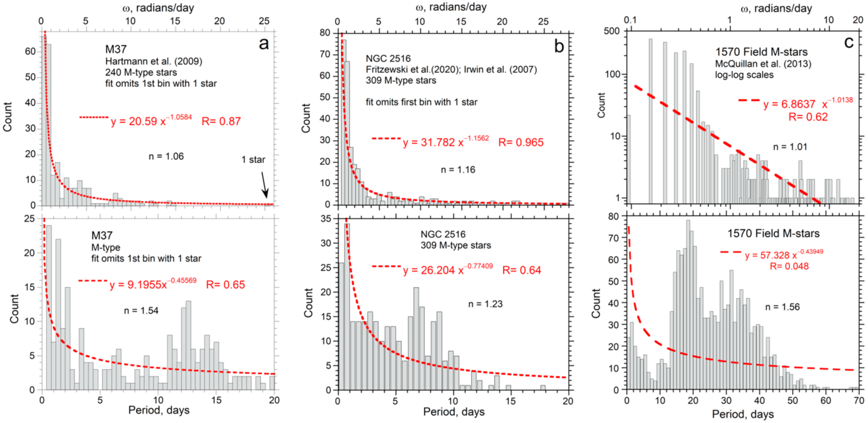
  • Periods of M stars in individual clusters behave similarly to the cluster as a whole (Figure 8a,b). Only M37 shows a peak at П = 12 d, which may represent episodic production. M37 is considered to be old and thus is most likely to depart from continuous production, since gas and dust are consumed with time.
In short, exponential spin-down describes M-type stars for any and all clusters, as well as M-types in star associations and in the Solar Neighborhood.

4.4.2. Type-K Stars

The most commonly sampled stars in missions previous to Kepler 2 are type-K’s. Histograms of K stars (Figure 13) have a secondary peak at П = 7 d. The corresponding broad peak expected at 0.9 radian d−1 in ω-histograms is not resolvable. Despite the moderate peak existing at П = 7 d, the overall best fit for both histograms on K-type stars is exponential decay (n~1). Cases n < ½ and n > 2 are ruled out.
To further explore the connection of histogram shape to mass, we constructed a histogram of small K-type stars (0.48 to 0.65 MSun; not shown). The appearance of the histogram pair for small type-K stars is intermediate to those of the M stars (Figure 11) and K stars (Figure 13), but with the weak and very broad peak at 7 days being split into two even weaker peaks at 5 and 10 days. For small K stars, decay is close to exponential, but as mass increases, a secondary peak develops which suggests a component of episodic production. Such episodic production causes departures of the measurements from n~1 behavior, since our mathematical analysis (Section 3) assumed constant production.
Because episodic production increases with mass, the largest K-types were not included in Figure 13. Instead, the largest K stars were grouped with type-G, discussed further below.

4.4.3. Type-G Stars

The clusters of Table 1 have varying numbers of type-G stars. To examine masses near solar and a large number of stars, Figure 14 includes the largest K’s and the smallest F’s in the clusters. The range of masses above and below solar is balanced in this manner, although very few F0-types were sampled. Despite production of these G stars having some episodic character, exponential decay of spin is supported.
Episodicity in production of large stars in the young cluster NGC 869 exists, but is slight. Unlike other young clusters of Table 1, solar mass stars constitute the largest fraction of measurements, and a statistically significant number of F-types were measured (Figure 15). Exponential decay describes the subgroups, recognizing that fitting period data with a peak and few data points typically gives n slightly larger than unity, and <1 for ω-histograms (not shown).

4.5. Laws Governing Spin Decay for MKG, and Probably F, Stars

Both ω-histograms and П-histograms for aggregated type-M and -K stars of all clusters in Table 1 combined are strongly skewed. This behavior also exists for type-M stars in individual clusters with many data points, except for old clusters (cf. Figure 3, Figure 5, Figure 7 and Figure 8), which have a peak in period that indicates some episodic production. The companion peak in ω-histograms is not resolved due to depopulation of the initial bins and/or the inverse relationship. Existence of a peak in П correlates with large stellar mass (Figure 14), suggesting that star production either becomes more episodic as mass increases or that production of the large stars slows with time. The former explanation is consistent with older cluster populations having a greater fraction of the larger type-G stars.
Small M stars do not show evidence of episodic production, except for the oldest cluster and for members of the Solar Neighborhood, which is circa 4.5 Ga, based on meteorite ages. For this reason, the best fits are found for clusters with many measurements of smaller stars (Figure 3 and Figure 5; Table 3).
The better match existing for small stars is attributed to their continuous production, consistent with their formation requiring only tiny volumes of gas and dust. The match for individual clusters, plus aggregated data on type-M and small K (Figure 11 and Figure 12) unequivocally rules out the exponents of n < 1/2 and n > 1.8 in Equations (18) and (20), and points to exponential decay of spin for the smallest dwarf stars. Even for older clusters or those with larger stars (Figure 5e,j,k), exponential decay is suggested by the data whereas n = 3 is ruled out. Skumanich’s 1972 proposal of n = 3 is inconsistent with the ω-histograms and completely incompatible with the П-histograms.

5. Mechanisms for Spin-Down

5.1. Fundamental Problems with the Magnetic Braking Hypothesis

Skumanich’s rule has found support in models of magnetic braking associated with ionized stellar winds (e.g., [78,79]). Regardless of whether flux or field strengths are considered, the principle underlying magnetic braking is that a moving charge experiences a sideways force (F) in a magnetic field (B) according to Lorentz’s force law:
F = qv × B
where v is the velocity vector and q is charge.
For two independent reasons, the net force (or torque) should be negligible on average:
  • Our Sun’s magnetic field reverses polarity every 11 years, which is accompanied by its sunspot cycle. Forces for the two polarities would act in opposite directions (21), thus providing alternate braking and acceleration. Hence, magnetic braking cancels magnetic acceleration over very short-term of 22 yr. This 22 yr cycle is unchanged over ~400 years of observations [80,81].
  • The sideways force depends on charge q, not on the mass of the charged particles. The stellar wind should be composed of roughly equal numbers of negatively and positively charged particles. Otherwise, the star would develop a net charge with time which then would preferentially retain the oppositely charged particles and restore charge balance. No net torques would arise.
Magnetic braking is not a feasible cause of spin-down if charge is conserved or if stars have reversals. Both behaviors are likely.

5.2. Viscous Dissipation as the Mechanism of Spin-Down

Viscous stress in a Newtonian fluid creates a force, F = Aμ∂vx/∂y where A = area, μ = the coefficient of viscosity, and flow is along the x direction [82]. The equatorial region dominates, so y ~ R, vx ~ Rω, and A is some function of R2, where R = radius. Using torque = R × F = I∂ω/∂t, where I = JMR2 and J is the reduced moment of inertia, and ∂ω/∂R = 0 for a solid body gives:
ω t = R F J M R 2 ~   R μ A J M R 2 ω ~   μ R J M ω ~ f ω  
which has the same form as Equation (7) for n = 1 and f = α. The function f combines the mass dependence of all variables.
Shear existing in stars is evident in the long-known latitudinal dependence of the rotation rate of our Sun, and also in the super-rotation of its core [83]. Differential rotation is also known in other stars: notably, part of the K2 mission was intended to explore differential rotation (e.g., [84]). Thus, viscous dissipation is a straightforward and logical explanation for progressive loss of stellar spin.

6. New Isochrones from Histogram Analysis

Quantifying spin-down using (7) requires both an initial angular velocity (or initial period) and a time constant for at least two stellar masses. We set limits, as follows.
The maximum initial spin rate is set by of the Virial Theorem, which relates gravitational potential energy (Ug) to rotational kinetic energy (R.E.):
2 R.E. spin = − Ug.
Equation (23) restricts the spin at formation for homogeneous density as:
ω0 = (2πρ0GN)½,
where GN is Newton’s gravitational constant [75]. Although internal densification has some effect (see [85] for examples including polytropes), constant density suffices for the present purposes.
Equation (24) provides П0 = 0.095 d for M = MSun which agrees with the fastest spinning type-G stars found in four different clusters (Figure 16). The t = 0 line must include the origin, since for null mass, the period is zero initially and remains zero for all time. Using the origin provides a linear equation for initial period of П0 = 0.095M/MSun days (Figure 16) which agrees with the fastest-spinning stars known [5,6]. The initial spin is also confirmed by Solar System trends [74,75]. Our t = 0 trend is further supported by the observation that many spin at slightly slower rates, denoted as the breakup velocity = (MG/R)½, e.g., [86].
The only information available to establish lifetime is the Sun’s current age (4.54 Ga) and period (24.5 d at the equator), which provide τ = 0.82 × 10⁹ yr. Consequently, we suggest the following dependence of period on age:
Π ( t ) = 0.095   days M M s u n p exp t 0.82   Ga
Combining the fit for density in Figure 1b with (24) suggests that power p = 0.57 (Figure 16c,d). This value assumes uniform density inside a star. We also consider p = 1 (Figure 16a,b). When M is near solar, p is immaterial. Thus, both cases for Equation (25) represent stars similar to our type-G2 Sun. As a first approximation, we assume (25) holds for main sequence M to F stars (Figure 16). Isochrones from (25) are thus defined by t = τ ln(П/П0).

6.1. Implications of Our Isochrones on Ages of Small Stars

Comparing Equation (25) to period data (Figure 16) shows that ages of main sequence dwarf stars in clusters mostly range from ~2 to 4.5 Ga. This finding is influenced by Kepler mission measurements of G-types being impacted by an upper limit of 25 to 32 days for reliable periods [60]. Ground-based measurements reach much larger П of 225 days [35] and indicate ages approaching 8 Ga for M-types if p = 1 or 7 Ga if p = 0.57, whereas the maximum ages for K and G stars observed from Mount Wilson (e.g., [36]) are less, ~5.5 Ga for either choice of p, as masses are near solar. Nearby stars are thus only a little older than the Sun. This finding is consistent with progressively larger stars having shorter life spans, as is well-known. Thus, our isochrones are supported by ground-based data.
Data on old open clusters are also consistent with the isochrones (Figure 16a). First, young stars are present only in Praesepe, which has the most measurements. Moreover, nebular gas is also absent, evolved stars exist, and the number of stars is few (Table 3). Finally, trends of period with mass for the oldest stars in evolved clusters which also have many measurements (Hyades, Praesepe, and NGC 6811) are parallel to the trend for ground-based data on the oldest, slowest stars (Figure 16a).
These parallel trends for the slowest star at any given mass describe destabilization of main sequence stars at old age. Destabilization at a certain period is explained qualitatively by fluid mechanics. Patterns of fluid flow in large rotating bodies depend on the relative effectiveness of inertial and Coriolis forces [82] so decreasing spin diminishes the latter, possibly triggering events which move the star off of the main sequence. Density and temperature both monotonically changing with mass (Figure 1b) are consistent with destabilization depending on mass.
Clusters with moderate model ages, all of which have white dwarfs (Table 1), also possess many young stars and rather few old stars (Figure 16b). Except for NGC 2516, a pile-up near the Sun’s position is not seen. This cluster also has fewer young stars than the others with similar model ages.
Clusters with young model ages and nebulae have many young stars, but also have ancient members of 4 Ga (Figure 16c). The trends of individual clusters are nearly parallel to the isochrons, particularly if p = 0.57, and so stellar demise is not evident in the period statistics. None of these clusters are described as having white dwarfs. Greater ages in Figure 16c than 16b is consistent with their population becoming older, but very few members have left the main sequence trend.
Figure 16d compares well-measured clusters with different ages to nearby field M-types and to Equation (25) with p = 0.57. The maximum age of 5.8 Ga for field M’s is greater than that of Praesepe members, with a parallel trend. Because the number of measurements in a restricted mass range is high (1570), McQuillan et al.’s [34] data reveal the maximum reliable periods for the Kepler missions. This maximum of ~50 days for 0.4 MSun is consistent with the reliability study of solar masses (<32 days [60]) and larger stars having shorter lifetimes. Ground-based measurements have large ages of 7 Ga for M-types (Figure 16a), corroborating that the maximum periods in the oldest clusters from Kepler mission datasets are underestimated. Maximum ages for the clusters in Figure 16b,c are not affected, because very few members reach the limits of measurable periods.
Because star ages are most accurate near the solar mass, Table 3 lists mean and maximum ages for the G-types. Because very fast rotators are under-represented in the measurements, Table 3 includes the minimum age for all stars in each group.

6.2. Implications of Our Isochrones on Ages and Evolution of Clusters

Cluster ages are estimated from trends in type-G ages (Table 3) as follows. The cluster must be at least as old as its oldest stars. Even the youngest, actively producing clusters have type-G stars with average ages near 3.3 Ga, as well as some old stars approaching 5 Ga. However, measurements cannot reliably resolve long periods and thus large ages. The ages of the oldest stars of any type in any cluster correlate roughly with age of its youngest star (Figure 17a). Because the upper age of stars involves the former demise of ancient population, the cluster age is set by adding 3 Ga to the age of the average G-type. The additive constant is based on the mean of 3.3 Ga for all clusters being close to half of the age of the oldest type-G star (5.3 Ga in the Mt Wilson group: Table 3).
The resulting age for the cluster is slightly greater than the oldest stars, which are almost always M-types (Figure 17a). This offset is consistent with periods being limited by the duration of the Kepler campaigns.
The clusters have similar ages (Table 3) because all are located in essentially the same part of the immense Milky Way (Table 1). The oldest clusters have little gas and few remaining stars, while the youngest clusters have nebulosity or molecular clouds and lack white dwarfs. These findings are supported by the weak correlations of star age with distance from the Sun (Figure 17b) and the scatter plot of star age with modeled cluster age (Figure 17c). Previous inferences of cluster age (Table 1) depend on modeled ages of their younger, large main sequence stars.

7. Conclusions

This paper provides an inverse method to extract the physical law governing the loss of star spin with time from histograms of spin period and its reciprocal, angular velocity. All available data on large open clusters that each have >120 measured light curves provide histogram pairs with similar shapes, indicating that exponential decay best describes spin-down of stars smaller than three Solar masses. Superimposed peaks in the ω- and П-histograms are attributed to episodic production. Skumanich’s formula and the previous gyrochronology model are contra-indicated. Our deduction of exponential spin-down is independent of the initial spin for the stars and is robust against the measurements being underpopulated for very short and very long periods.
If coeval production of all stars in open clusters is assumed, our forward models yield histogram shapes that are unlike any observed, regardless of what rate law is considered. The replacement of a coeval theory for star production with one assuming steady state production of small stars is parallel with the catastrophism vs. uniformitarianism dilemma faced by pioneer geologists (ca. 1785 to 1830), with the latter explanation ultimately prevailing for numerous processes.
Importantly, period measurements are made of small stars on the main sequence, which describes these dwarfs over most of their lifetime, while the star is stable. The exponential rate law likely applies to all stable stars of any size. The associated time constant probably depends on mass, but ascertaining this is beyond the scope of the present report.
Diverse phenomena are controlled by exponential attenuation, such as absorption of light by matter, radioactive decay, heat flow (Newton’s law of cooling), capacitor discharge, or vibrational damping. Based on exponential spin-down, we constructed isochrones using the known age of the Sun and its estimated initial spin (Figure 16). Our isochrones are most accurate for stars with ages of several billion years and masses near or slightly below solar.

7.1. Astrophysical Implications

Figure 16d suggests that type-B6 stars can attain much greater ages than previously considered. Additional statistical analysis of data on large stars would be useful, and is possible using Doppler measurements. Nonetheless, the trend suggests a resolution to the puzzle as to how a young, large B8-O0 star could orbit an old black hole [87]. Specifically, the orbiter could be far older than assumed.
The Sun spins slowly compared to those near-solar-mass stars in open clusters and nearby regions of the Milky Way (Table 1 lists the many studies). This fact, combined with histogram analyses of the present report, points to it not being middle-aged as commonly assumed (Figure 3, Figure 4, Figure 5, Figure 6, Figure 7, Figure 8, Figure 9, Figure 14 and Figure 16). The Sun numbers among the oldest type-G stars (Figure 17). From the Mt. Wilson study, maximum ages of G-types increase from 5 to 5.6 Ga as mass decreases (Figure 16a). Our finding, combined with the 4.5 Ga time-span on Earth for humanoids to develop, offers a resolution to Fermi’s paradox. Namely, the requirement for star longevity coupled with planet habitability significantly reduces the frequency of possible civilizations.

7.2. General Applicability

Histograms are commonly used to represent a key variable of a population. Our mathematical formulation can be applied to other phenomena. The variable does not need not be angular momentum, or even to have a meaningful reciprocal (e.g., period), but can be any physical attribute. The limitation is that the primary variable must be described by a power law similar to Equation (7), which covers many possibilities, since n can be non-integer. Note that the independent variable does not need to be time.

Author Contributions

Methodology, R.E.C.; validation, A.M.H. All other aspects of were shared equally. All authors have read and agreed to the published version of the manuscript.

Funding

This research received no external funding.

Acknowledgments

We thank Sandor Frey for inviting this submission.

Conflicts of Interest

The authors declare no conflict of interest.

References

  1. Soderblom, F.T. The ages of stars. Ann. Rev. Astron. Astrophys. 2010, 48, 581–629. [Google Scholar] [CrossRef] [Green Version]
  2. Strobel, N. Astronomy Notes; XanEdu: Ann Arbor, MI, USA, 2020. [Google Scholar]
  3. Amand, L.; Palacio, A.; Charbonnel, C.; Gallet, F.; Georgy, C.; Lagarde, N.; Siess, L. First grids of low-mass stellar models and isochrones with self-consistent treatment of rotation from 0.2 to 1.5M at seven metallicities from PMS to TAMS. Astron. Astro. 2019, 631, A77. [Google Scholar] [CrossRef] [Green Version]
  4. Gilmour, J. The extinct radionuclide timescale of the early solar system. Space Sci. Rev. 2000, 92, 123–132. [Google Scholar] [CrossRef]
  5. Dufton, P.L.; Dunstall, P.R.; Evans, C.J.; Brott, I.; Cantiello, M.; De Koter, A.; de Mink, S.; Fraser, M.; Hénault-Brunet, V.; Howarth, I.D.; et al. The VLT-FLAMES tarantula survey: The fastest rotating O-type star and shortest period LMC pulsar—remnants of a supernova disrupted binary? Astrophys. J. 2011, 743, L22. [Google Scholar] [CrossRef] [Green Version]
  6. Müller, A.; van den Ancker, M.E.; Launhardt, R.; Pott, J.U.; Fedele, D.; Henning, T. HD 135344B: A young star has reached its rotational limit. Astron. Astrophys. 2011, 530, A85. [Google Scholar] [CrossRef]
  7. Skumanich, A. Time scales for Ca II emission decay, rotational braking, and lithium depletion. Astrophys. J. 1972, 171, 565–567. [Google Scholar] [CrossRef]
  8. Terndrup, D.M.; Stauffer, J.R.; Pinsonneault, M.H.; Sills, A.; Yuan, Y.; Jones, B.F.; Fischer, D.; Krishnamurthi, A. Rotational velocities of low-mass stars in the Pleiades and Hyades. Astrophys. J. 2000, 119, 1303–1316. [Google Scholar] [CrossRef] [Green Version]
  9. Strassmeier, K.G. Starspots. Astron. Astrophys. Rev. 2009, 17, 251–308. [Google Scholar] [CrossRef] [Green Version]
  10. Finley, A.J.; Hewitt, A.L.; Matt, S.P.; Owers, M.; Pinto, R.F.; Veville, V. Direct detection of solar angular momentum loss with the Wind spacecraft. Astrophys. J. Lett. 2019, 885, L30. [Google Scholar] [CrossRef] [Green Version]
  11. Angus, R.; Morton, T.D.; Foreman-Mackey, D.; Van Saders, J.; Curtis, J.; Kane, S.R.; Bedell, M.; Kiman, R.; Hogg, D.W.; Brewer, J. Toward precise stellar ages: Combining isochrone fitting with empirical gyrochronology. Astron. J. 2019, 158, 173. [Google Scholar] [CrossRef]
  12. Chandrasekhar, S.; Münch, G. On the integral equation governing the distribution of the true and apparent rotational velocities of stars. Astrophys. J. 1950, 111, 142–156. [Google Scholar] [CrossRef]
  13. Henderson, C.B.; Stassun, K.G. Time-series photometry of stars in and around the Lagoon nebula. I. Rotation periods of 290 low-mass pre-main-sequence stars in NGC 6530. Astrophys. J. 2012, 747, 51. [Google Scholar] [CrossRef] [Green Version]
  14. Lamm, M.; Mundt, H.R.; Bailer-Jones, C.A.L.; Herbst, W. Rotational evolution of low mass stars: The case of NGC 2264. Astron. Astrophys. 2012, 430, 1005–1026. [Google Scholar] [CrossRef]
  15. Littlefair, S.P.; Naylor, T.; Mayne, N.J.; Saunders, E.S.; Jeffries, R.D. Rotation of young stars in Cepheus OB3b. Mon. Not. R. Astron. Soc. 2010, 403, 545–557. [Google Scholar] [CrossRef] [Green Version]
  16. Irwin, J.; Hodgkin, J.S.; Aigrain, S.; Bouvier, J.; Hebb, L.; Irwin, M.; Moraux, E. The Monitor project: Rotation of low-mass stars in NGC 2362—testing the disc regulation paradigm at 5 Myr. Mon. Not. R. Astron. Soc. 2008, 384, 675–686. [Google Scholar] [CrossRef] [Green Version]
  17. Moraux, E.; Artemenko, S.; Bouvier, J.; Irwin, J.; Ibrahimov, M.; Magakian, T.; Grankin, K.; Nikogossian, E.; Cardoso, C.; Hodgkin, S.; et al. The Monitor project: Stellar rotation at 13 Myr. Astron. Astrophys. 2013, 560, A13. [Google Scholar] [CrossRef] [Green Version]
  18. Irwin, J.; Hodgkin, S.; Aigrain, S.; Bouvier, J.; Hebb, L.; Moraux, E. The Monitor project: Rotation of low-mass stars in the open cluster NGC 2547. Mon. Not. R. Astron. Soc. 2008, 383, 1588–1602. [Google Scholar] [CrossRef] [Green Version]
  19. Irwin, J.; Aigrain, S.; Bouvier, J.; Hebb, L.; Hodgkin, S.; Irwin, M.; Moraux, E. The Monitor project: Rotation periods of low-mass stars in M50. Mon. Not. R. Astron. Soc. 2009, 392, 1456–1466. [Google Scholar] [CrossRef] [Green Version]
  20. Hartman, J.D.; Bakos, G.A.; Kovacs, G.; Noyes, R.W. A large sample of photometric rotation periods for FGK Pleiades stars. Mon. Not. R. Astron. Soc. 2010, 408, 475–489. [Google Scholar] [CrossRef] [Green Version]
  21. Rebull, L.M.; Stauffer, J.R.; Bouvier, J.; Cody, A.M.; Hillenbrand, L.A.; Soderblom, D.R.; Valenti, J.; Barrado, D.; Bouy, H.; Ciardi, D.; et al. Rotation in the Pleiades with K2. I. Data and first results. Astron. J. 2016, 152, 113. [Google Scholar] [CrossRef] [Green Version]
  22. Covey, K.R.; Agueros, M.A.; Law, N.M.; Liu, J.; Ahmadi, A.; Laher, R.; Levitan, D.; Sesar, B.; Surace, J. Why are rapidly rotating M dwarfs in the Pleiades so (infra) red? New period measurements confirm rotation-dependent color offsets from the cluster sequence. Astrophys. J. 2016, 822, 81. [Google Scholar] [CrossRef]
  23. Meibom, S.; Mathieu, R.D.; Stassun, K.G. Stellar rotation in M35: Mass–period relations, spin-down rates, and gyrochronology. Astrophys. J. 2009, 695, 679–694. [Google Scholar] [CrossRef]
  24. Fritzewsky, D.J.; Barnes, S.A.; James, D.J.; Strassmeier, K.G. The rotation period distribution of the rich Pleiades-age southern open cluster NGC2516. Aston. Astrophys. 2020, 641, A51. [Google Scholar] [CrossRef]
  25. Irwin, J.; Hodgkin, S.; Aigrain, S.; Hebb, L.; Bouvier, J.; Clark, C.; Moraux, E.; Bramich, D.M. The Monitor project: Rotation of low-mass stars in the open cluster NGC 2516. Mon. Not. R. Astron. Soc. 2007, 377, 741–755. [Google Scholar] [CrossRef] [Green Version]
  26. Meibom, S.; Mathieu, R.D.; Stassun, K.G.; Liebesny, P.; Saar, S.H. The color–period diagram and stellar rotational evolution—new rotation period measurements in the open cluster M34. Astrophys. J. 2011, 733, 115. [Google Scholar] [CrossRef] [Green Version]
  27. Hartman, J.D.; Gaudi, B.S.; Holman, M.J.; McLeod, B.A.; Stanek, K.Z.; Barranco, J.A.; Pinsonneault, M.H.; Kalirai, J.S. Deep MMT transit survey of the open cluster M37. II. Variable stars. Astrophys. J. 2009, 675, 1254–1277. [Google Scholar] [CrossRef] [Green Version]
  28. Douglas, S.T.; Curtis, J.L.; Agüeros, M.A.; Cargile, P.A.; Brewer, J.M.; Meibom, S.; Jansen, T. K2 Rotation periods for low-mass Hyads and a quantitative comparison of the distribution of slow rotators in the Hyades and Praesepe. Astrophys. J. 2019, 879, 100. [Google Scholar] [CrossRef]
  29. Douglas, S.T.; Agüeros, M.A.; Covey, K.R.; Kraus, A. Poking the beehive from space: K2 rotation periods for Praesepe. Astrophys. J. 2017, 842, 83. [Google Scholar] [CrossRef] [Green Version]
  30. Curtis, J.L.; Agüeros, M.A.; Douglas, S.T.; Meibom, S. A temporary epoch of stalled spin-down for low-mass stars: Insights from NGC 6811with Gaia and Kepler. Astrophys. J. 2019, 879, 49. [Google Scholar] [CrossRef]
  31. Mellon, S.N.; Mamajek, E.E.; Oberst, T.E.; Pecaut, M.J. Angular momentum evolution of young stars in the nearby Scorpius–Centaurus OB Association. Astrophys. J. 2017, 844, 66. [Google Scholar] [CrossRef] [Green Version]
  32. Gagne, J.; David, T.J.; Mamajek, E.E.; Manon, A.W.; Faherty, J.K.; Bedard, A. The μ Tau Association: A 60 Myr old coeval group at 150 pc from the Sun. Astrophys. J. 2020, 903, 96. [Google Scholar] [CrossRef]
  33. Saylor, D.; Lepine, S.; Crossfield, I.; Petigura, E. Light-curve modulation of low-mass stars in K2. I. Identification of 481 fast rotators in the Solar Neighborhood. Astrophys. J. 2018, 155, 23. [Google Scholar]
  34. McQuillan, A.; Aigrain, S.; Mazeh, T. Stellar rotation periods of the Kepler objects of interest: A dearth of close-in planets around fast rotators. Mon. Not. R. Astron. Soc. 2013, 432, 1203–1216. [Google Scholar] [CrossRef] [Green Version]
  35. Newton, E.R.; Mondrik, N.; Irwin, J.; Winters, J.G.; Charbonneau, D. New rotation period measurements for M Dwarfs in the Southern Hemisphere: An abundance of slowly rotating, fully convective stars. Astron. J. 2018, 156, 217. [Google Scholar] [CrossRef]
  36. Baliunas, S.; Sokoloff, D.; Soon, W. Magnetic field and rotation in lower main-sequence stars: An empirical time-dependent magnetic Bode’s relation? Astrophys. J. 1996, 457, L99–L102. [Google Scholar] [CrossRef] [Green Version]
  37. Pecaut, M.C.; Mamajec, E.E. Intrinsic colors, temperatures, and bolometric corrections of pre-main-sequence stars. Astrophys. J. Supp. 2013, 208, 9. [Google Scholar] [CrossRef]
  38. Zombeck, M.V. Handbook of Space Astronomy and Astrophysics; Cambridge Univ. Press: Cambridge, UK, 2007; pp. 105–109. [Google Scholar]
  39. Leonard, P.J.T.; Merritt, D. The mass of the open star cluster M35 as derived from proper motions. Astrophys. J. 1989, 339, 195–208. [Google Scholar] [CrossRef]
  40. Barrado y Navascués, D.; Stauffer, J.R.; Bouvier, J.; Martín, E.L. From the top to the bottom of the main sequence: A complete mass function of the young open cluster M35. Astrophys. J. 2001, 546, 1006–1018. [Google Scholar] [CrossRef] [Green Version]
  41. Moraux, E.; Bouvier, J.; Stauffer, J.R.; Cuillandre, J.C. Brown dwarfs in the Pleiades cluster: Clues to the substellar mass function. Astron. Astrophys. 2003, 400, 891–902. [Google Scholar] [CrossRef] [Green Version]
  42. Moraux, E.; Kroupa, P.J.; Bouvier, J. The Pleiades mass function: Models versus observations. Astron. Astrophys. 2004, 426, 75–80. [Google Scholar] [CrossRef] [Green Version]
  43. Bouvier, J.; Kendall, T.; Meeus, G.; Testi, L.; Moraux, E.; Stauffer, J.R.; James, D.; Cuillandre, J.-C.; Irwin, J.; McCaughrean, M.J.; et al. Brown dwarfs and very low mass stars in the Hyades cluster: A dynamically evolved mass function. Astron. Astrophys. 2008, 481, 661–672. [Google Scholar] [CrossRef]
  44. Williams, D.M.; Rieke, G.H.; Stauffer, J.R. The stellar mass function of praesepe. Astrophys. J. 1995, 445, 359–366. [Google Scholar] [CrossRef]
  45. Wang, W.; Boudreault, S.; Goldman, B.; Henning, T.; Caballero, J.A.; Bailer-Jones, C.A.L. The substellar mass function in the central region of the open cluster Praesepe from deep LBT observations. Astron. Astrophys. 2011, 531, A164. [Google Scholar] [CrossRef]
  46. Transtrum, M.K.; Machta, B.B.; Brown, K.S.; Daniels, B.C.; Myers, C.R.; Sethna, J.P. Perspective, sloppiness and emergent theories in physics, biology, and beyond. J. Chem. Phys. 2015, 143, 010901. [Google Scholar] [CrossRef] [PubMed]
  47. Groetsch, C.W. Inverse Problems: Activities for Undergraduates; Cambridge University Press: Cambridge, UK, 1999. [Google Scholar]
  48. Kirsch, A. An Introduction to the Mathematical Theory of Inverse Problems; Springer: New York, NY, USA, 1966. [Google Scholar]
  49. Armbartsumian, V. On the derivation of the frequency function of space velocities of the stars from the observed radial velocities. Mon. Not. R. Astron. Soc. 1936, 96, 172–178. [Google Scholar]
  50. Criss, R.E.; Hofmeister, A.M. Density Profiles of 51 galaxies from parameter-free inverse models of their measured rotation curves. Galaxies 2020, 8, 19. [Google Scholar] [CrossRef] [Green Version]
  51. Apostol, T.M. Calculus: Multi-variable Calculus and Linear Algebra, with Applications to Differential Equations and Probability; Xerox College Publishing: Waltham, MA, USA, 1969. [Google Scholar]
  52. Jackson, R.J.; Jeffries, R.D. Chromospheric activity among fast-rotation M dwarfs in the open cluster NGC 2516. Mon. Not. R. Astron. Soc. 2010, 407, 465–478. [Google Scholar] [CrossRef] [Green Version]
  53. Douglas, S.T.; Agüeros, M.A.; Covey, K.R.; Cargile, P.A.; Barclay, T.; Cody, A.; Howell, S.B.; Kopytova, T. K2 rotation periods for low-mass Hyads and the implications for gyrochronology. Astrophys. J. 2016, 822, 47. [Google Scholar] [CrossRef] [Green Version]
  54. Cui, K.; Liu, J.; Yang, S.; Gao, Q.; Yang, H.; Soria, R.; He, L.; Wang, S.; Bai, Y.; Yang, F. Long rotation period main-sequence stars from Kepler SAP light curves. Mon. Not. R. Astron. Soc. 2019, 413, 2218–2234. [Google Scholar] [CrossRef] [Green Version]
  55. McQuillan, A.; Mazeh, T.; Aigrain, S. Rotation periods of 34,030 Kepler main-sequence stars: The full autocorrelation sample. Astrophys. J. Suppl. Ser. 2014, 211, 24. [Google Scholar] [CrossRef] [Green Version]
  56. Affer, L.; Micela, G.; Favata, F.; Flaccomio, E.; Bouvier, J. Rotation in NGC 2264: A study based on CoRoT photometric observations. Mon. Not. R. Astron. Soc. 2013, 430, 1433–1446. [Google Scholar] [CrossRef] [Green Version]
  57. Scholz, A.; Eislöffel, J.; Mundt, R. Long-term monitoring in IC4665: Fast rotation and weak variability in very low mass objects. Astron. Astrophys. 2009, 400, 1548–1562. [Google Scholar] [CrossRef] [Green Version]
  58. James, D.J.; Barnes, S.A.; Meibom, S.; Lockwood, G.W.; Levine, S.E.; Deliyannis, C.; Platais, I.; Steinhauer, A.; Hurley, B.K. New rotation periods in the open cluster NGC 1039 (M34), and a derivation of its gyrochronology age. Astron. Astrophys. 2010, 515, A100. [Google Scholar] [CrossRef]
  59. Reiners, A.; Joshi, N.; Goldman, B. A catalog of rotation and activity in early-M stars. Astrophys. J. 2012, 143, 93. [Google Scholar] [CrossRef] [Green Version]
  60. Esselstein, R.; Aigrain, S.; Vanderburg, A.; Smith, J.C.; Meibom, S.; Van Saders, J.; Mathieu, R. The K2 M67 study: Establishing the limits of stellar rotation period measurements in M67 with K2 campaign 5 cata. Astrophys. J. 2018, 859, 167. [Google Scholar] [CrossRef] [Green Version]
  61. Finlay, W.H. Concise Catalog of Deep-Sky Objects; Springer: London, UK, 2003. [Google Scholar]
  62. Kraft, R.P. Studies of Stellar Rotation. V. The dependence of rotation on age among solar-type stars. Astrophys. J. 1967, 150, 551–571. [Google Scholar] [CrossRef]
  63. Soderblom, F.T. Rotational studies of late-type stars. II—Ages of solar-type stars and the rotational history of the Sun. Astrophys. J. Suppl. Ser. 1982, 53, 1–15. [Google Scholar] [CrossRef]
  64. Barnes, S.A. On the rotational evolution of solar- and late-type stars, its magnetic origins, and the possibility of stellar gyrochronology. Astrophys. J. 2003, 586, 464–479. [Google Scholar] [CrossRef] [Green Version]
  65. Barnes, S.A. Ages for illustrative field stars using gyrochronology: Viability, limitations, and errors. Astrophys. J. 2007, 669, 1167–1189. [Google Scholar] [CrossRef] [Green Version]
  66. Cargile, P.A.; James, D.L.; Pepper, J.; Kuhn, R.B.; Siverd, R.; Stassun, K.G. Evaluating gyrochronology on the zero-age-main-sequence: Rotation periods in the southern open cluster Blanco 1 from the Kelt-south survey. Astrophys. J. 2014, 782, 29. [Google Scholar] [CrossRef] [Green Version]
  67. Epstein, C.R.; Pinsonneault, M.H. How good a clock is rotation? The stellar rotation–mass–age relationship for old field stars. Astrophys. J. 2014, 780, 159. [Google Scholar] [CrossRef] [Green Version]
  68. Twarog, B.A.; Carraro, G.; Anthony-Twarog, B.J. Evidence for extended star formation in the old, metal-rich open cluster, NGC 6791? Astrophys. J. Lett. 2011, 727, L7. [Google Scholar] [CrossRef]
  69. Geisler, D.; Villanova, S.; Carraro, G.; Pilachowski, C.; Cummings, J.; Johnson, C.I.; Bresolin, F. The unique Na: Abundance distribution in NGC 6791: The first open(?) cluster with multiple populations. Astrophys. J. Lett. 2012, 756, L40. [Google Scholar] [CrossRef] [Green Version]
  70. Van Saders, J.L.; Pinsonneault, M.H.; Barbieri, M. Forward modeling of the Kepler stellar rotation period distribution: Interpreting periods from mixed and biased stellar populations. Astrophys. J. 2019, 872, 128. [Google Scholar] [CrossRef] [Green Version]
  71. Bevington, P.R. Data Reduction and Error Analysis for the Physical Sciences; McGraw-Hill: New York, NJ, USA, 1969. [Google Scholar]
  72. Collier Cameron, A.; Davidson, V.A.; Hebb, L.; Skinner, G.; Anderson, D.R.; Christian, D.J.; Clarkson, W.I.; Enoch, B.; Irwin, J.; Joshi, Y.; et al. The main-sequence rotation–Colour relation in the Coma Berenices open cluster. Mon. Not. R. Astron. Soc. 2009, 400, 451–462. [Google Scholar] [CrossRef] [Green Version]
  73. Kovács, G.; Hartman, J.D.; Bakos, G.A.; Quinn, S.N.; Penev, K.; Latham, D.W.; Bhatti, W.; Csubry, Z.; de Val-Borro, M. Stellar rotation periods in planet hosting open cluster Praesepe. Mon. Not. R. Astron. Soc. 2014, 442, 2081–2093. [Google Scholar] [CrossRef] [Green Version]
  74. Hofmeister, A.M.; Criss, R.E. A thermodynamic model for formation of the Solar System via 3-dimensional collapse of the dusty nebula. Planet. Space Sci. 2012, 62, 111–131. [Google Scholar] [CrossRef]
  75. Hofmeister, A.M.; Criss, R.E. Spatial and symmetry constraints as the basis of the virial theorem and astrophysical implications. Can. J. Phys. 2016, 94, 380–388. [Google Scholar] [CrossRef]
  76. Delorme, P.; Collier Cameron, A.; Hebb, L.; Rostron, J.; Lister, T.A.; Norton, A.J.; Pollacco, S.; West, R.G. Stellar rotation in the Hyades and Praesepe: Gyrochronology and braking time-scale. Mon. Not. R. Astron. Soc. 2011, 413, 2218–2234. [Google Scholar] [CrossRef] [Green Version]
  77. Meibom, S.; Barnes, S.A.; Latham, D.W.; Batalha, N.; Borucki, W.J.; Koch, D.G.; Basri, G.; Walkowicz, L.M.; Janes, K.A.; Jenkins, J.; et al. The Kepler cluster study: Stellar rotation in NGC 6811. Astrophys. J. Lett. 2011, 733, L9. [Google Scholar] [CrossRef]
  78. Bouvier, J.; Forestini, M.; Allain, S. The angular momentum evolution of low-mass stars. Astron. Astrophys. 1997, 326, 1023–1043. [Google Scholar]
  79. Reiners, A.; Mohanty, S. Radius-dependent angular momentum evolution in low-mass stars. I. Astrophys. J. 2012, 746, 43. [Google Scholar] [CrossRef] [Green Version]
  80. SILSO. World Data Center—Sunspot Number and Long-Term Solar Observations from the Royal Observatory of Belgium, on-Line Sunspot Number Catalogue. Covering 1749 to 2020. Available online: http://www.sidc.be/silso/datafiles (accessed on 16 May 2020).
  81. Hoyt, D.V.; Schatten, K.H. Group sunspot numbers: A new solar activity reconstruction. Part 2. Solar Phys. 1998, 181, 491–512. [Google Scholar] [CrossRef]
  82. Tritton, D.J. Physical Fluid Dynamics; Van Nostrand Reinhold Co.: New York, NY, USA, 1977. [Google Scholar]
  83. Fossat, E.; Boumier, P.; Fossat, E.; Corbard, T.; Provost, J.; Salabert, D.; Schmider, F.X.; Gabriel, A.H.; Grec, G.; Renaud, C.; et al. Asymptotic g modes: Evidence for a rapid rotation of the solar core. Astron. Astrophys. 2017, 604, A40. [Google Scholar] [CrossRef] [Green Version]
  84. Karoff, C.; Metcalfe, T.S.; Chaplin, W.J.; Elsworth, Y.; Kjeldsen, H.; Arentoft, T.; Buzasi, D. New rotation periods in the open cluster NGC 1039 (M 34), and a derivation of its gyrochronology age. Mon. Not. R. Astron. Soc. 2009, 399, 914–923. [Google Scholar] [CrossRef] [Green Version]
  85. Hofmeister, A.M.; Criss, R.E. Implications of geometry and the theorem of Gauss on Newtonian gravitational systems and a caveat regarding Poisson’s equation. Galaxies 2017, 5, 89–100. [Google Scholar] [CrossRef] [Green Version]
  86. Slettebak, A. On the axial rotation of brighter O and B stars. Astrophys. J. 1949, 110, 498–514. [Google Scholar] [CrossRef]
  87. Ghez, A.M.; Duchêne, G.; Matthews, K.; Hornstein, S.D.; Tanner, A.; Larkin, J.; Morris, M.; Becklin, E.E.; Salim, S.; Kremenek, T.; et al. The first measurement of spectral lines in a short-period star bound to the galaxy’s central black hole: A paradox of youth. Astrophys. J. 2003, 586, L127–L131. [Google Scholar] [CrossRef]
Figure 1. Cluster and star properties vs. normalized star mass: (a) Observed star fractions in well–studied open clusters. Stellar types are shown on the upper axis. Curves are to guide the eye. Dots and heavy curve = M35 [39,40]. Open squares and fine curve = Pleiades [41,42]. Grey triangles and grey curve = Hyades [43]. Filled diamonds and dashed = Praesepe [44,45]; (b) Density (red color and left axis) and blackbody temperature (blue color and right axis) of main sequence stars. Symbols are the values listed in the summary tables of Zombeck [38]. Lines are least square fits of each dataset assuming a power law dependence on mass: each line is labeled with its fits. Horizontal lines show ambient densities for select materials. Main sequence star classifications (labels M8 to O5) are based on color which encapsulates all properties, except spin, of main sequence stars.
Symmetry 13 01519 g001
Figure 2. Gyrochronology models: (a) Scatter plot of star rotation period vs. their B-V spectroscopic character for 3 different datasets on the Pleiades cluster, showing that the C- and I-trends from 2003 [64] are not supported by larger, subsequent data sets [20,21]. Upper x-axis shows star mass. This graph has no connection with star age; (b) Comparison of data on periods near 0.3 MSun to the I- and C-trends, calculated using Equations (5) and (6) with model cluster ages. Various symbols show individual clusters, see Table 1 for details. Pleiades stars are black cross symbols; (c) As above, but for 1 solar mass. These plots provide no support for Equations (5) and (6).
Symmetry 13 01519 g002
Figure 3. Histograms of angular velocity (top) and periods (bottom) for the well-studied Pleiades cluster have similar shapes: (a) The first large datasets on Pleiades open cluster [20]; (b) Data obtained during a recent mission [21], where the points are plotted at the top center of each bin; (c) A study focused on small, fast-spinning stars [22]. Histogram bins are shown as a symbol at the top of the bin in its middle. Black curve = least squares fit with the fit as indicated and n from the model developed in Section 3. If stated, the de-populated first bin was omitted in fitting.
Symmetry 13 01519 g003
Figure 4. Theoretical time evolution of histograms for a group of coeval stars with random initial spins, up to a normalized upper limit: (left) = histogram of 1000 stars with random initial spins; (middle) = histograms after moderate time has elapsed (αt = 0.4) for exponential decay (top) and Skumanich’s rule (bottom); (right) = histograms after significant time has elapsed (αt = 1) for the same n values. No measurement set provides similar shapes (see Figure 3 and Figure 5).
Symmetry 13 01519 g004
Figure 5. Paired histograms for all individual open clusters with >170 measurements on small stars, excluding the Pleiades. See Figure 3 for symbols and Pleiades data. All but two clusters (parts f,l) have >243 data points. Clusters are ordered from (al) using previous models for cluster age, listed in Table 1, along with data sources of spin. Panels (a,d,i,l) show the histograms in gray.
Symmetry 13 01519 g005aSymmetry 13 01519 g005b
Figure 6. Paired histograms of clusters with ~125 members. Symbols as in Figure 5: (a) Hyades, for which data from [28] are highly accurate and cover a wide range of periods; (b) M34 data from [26], which sampled K- and G-types, with few periods exceeding 15 days.
Symmetry 13 01519 g006
Figure 7. Effect of bin size on determinations of the power law exponent. The four largest datasets of Table 1 were explored as these allow examination of the largest range in bin size. Least squares fits are shown. All evaluations point to n~1: (a) Data from [31]; (b) Data from [21]; (c) Data from [19]; (d) Data from [29].
Symmetry 13 01519 g007
Figure 8. Fits for M-type stars. Symbols described in Figure 5: (a) M37 (data from [27]) has a peak at 12 days, but is fit reasonably well; (b) NGC 2516 (data from [24]) has more M-types, in number and proportion, but this distribution also have a peak; (c) Small field stars close to the Sun: data from [34]. Note that the angular momentum panel is on a log-log scale. These stars are not related, need not be produced continuously, and their distribution is poorly represented by a power law.
Symmetry 13 01519 g008
Figure 9. Histograms of recently measured associations of stars. Panels are ordered by increasing sample size. Symbols as in Figure 5: (a) Pre-main sequence stars of the Scorpious-Centaurus OB association from [31]; (b) A wide range of masses in the μ Tau association, which includes a B2 star and pre-main sequence stars [32]. Arrow points to the slow rotator; (c) Fast rotators in the Solar Neighborhood [33]. Adding the Sun makes little difference to the fits.
Symmetry 13 01519 g009
Figure 10. Histograms of ground-based observations. Symbols as in Figure 5: (a) Nearby M stars in the Southern Hemisphere [35] possess a unique distribution; (b) Compilation [36] of long-standing data on well-characterized stars.
Symmetry 13 01519 g010
Figure 11. Histogram pairs for aggregated M-type stars (M < 0.48Msun). Fits shown in this plot assumed various, fixed values for n in (17) and (19), as labeled. Counts for bins near the origin not included in fitting are indicated. Exponential decay (n = 1) provides the best fit for both visualizations.
Symmetry 13 01519 g011
Figure 12. Numerical analysis of histogram data using (18) and (20). Dots = count in Figure 11 for M-types: (a) Analysis of ω-histograms using bin size of 0.5 radians/day. By plotting count against 1/ω, the under-populated initial bins (open symbols) can be excluded from the fit, and young stars are emphasized; (b) Analysis of П-histograms using a bin size of 0.5 days. Bin #1 is off scale with N = 8 and 1/П = 11 d−1. This approach does not assume that ω (or П) is large compared to bin size. The linear trends show that spin attenuation is exponential (n = 1).
Symmetry 13 01519 g012
Figure 13. Histograms for K-type stars (0.48 < M/Msun < 0.8). The largest K stars (0.8 to 0.9 solar masses are excluded, see text. Fits shown in this plot assumed various, fixed values for n in Equations (18) and (20), as labeled. Counts for bins near the origin not included in fitting are indicated. No curves provide optimal fits due to episodic production, particularly for M37. Nonetheless, the two plots constrain ~1/2 < n < 2.
Symmetry 13 01519 g013
Figure 14. Combined histograms of light curve data on angular velocity (left) and periods (right) for mostly G-type stars. A mass range of 0.8 < M/MSun < 1.2 was used for balance. Fits shown in this plot assumed various, fixed values for n in (18) and (20), as labeled. Counts for bins near the origin not included in fitting are indicated. Coefficients are shown for the exponential case (red curves and text. None of the fits are optimal due to episodic production. However, n ≥ 2 can be ruled out based on period data. For angular velocity, n from 1 to 2 provides the best fits. The best fits to a floating power are: n = 0.74 for П and n = 1.37 for ω.
Symmetry 13 01519 g014
Figure 15. Period histograms of large star types in NGC 869. Only 56 M-types (0.32 to 0.48 MSun) were measured [17], which are too few for a statistical analysis: (a) Masses from 0.48 to 0.8 solar; (b) Masses from 0.8 to 1.2 solar; (c) Masses from 1.2 to 1.5 solar. No larger stars were measured.
Symmetry 13 01519 g015
Figure 16. Period data vs. normalized mass of stars compared to our isochrons. For all panels, individual clusters are colored. Black symbols are reference points: square in circle = the Sun and a “young” Herbig object [6]. Solid lines = proposed isochrones, ages as labeled, where the upper panels consider p = 1 in (24) while the lower use p = 0.57. Dotted line = initial spin from the Virial theorem (see text) which is confirmed by the Herbig object and the fastest known O-star, with M = 22Msun and a period of 0.88 days [5]. Heavy red arrow on the upper axis indicates a typical observational cutoff. Stars in any open cluster have many ages: (a) Open clusters considered to be old, plus 29 stars in Coma Berenices (red-brown dots) [72] and 30 slow rotators in M67 (light pink dots) [60]; (b) Clusters with moderate model ages. Most stars are ~3 Ga old, which a substantial portion of young stars, and some evidence for stellar demise in NGC 2516, which lacks fast rotators; (c) Clusters with young ages, plus data on 20 fast rotators in the young cluster IC4665 (pale blue-gray triangles) [57]. The average age is near 4 Ga, and no evidence exists for stellar demise; (d) Comparison of one large dataset for each of old, moderate, and young model ages to field M-types (grey dots). Note that the x-axis is shifted from that in the other panels. The trend for field stars [34] indicates that periods of M-types in the missions are limited to 40-60 days. Large green dots = data on 3 Be stars in Pleiades, which are consistent with the young ages of smaller members.
Symmetry 13 01519 g016
Figure 17. Graphical representation of the various ages from Table 3, with the addition of the maximum for M-types using p = 1: (a) Dependence of various star ages on the age of the youngest star in each group or cluster. Convergence of the average (black dots) and oldest (open squares) type-G stars at ~4.5 Ga is consistent with constant production until nebula gas runs out and G stars die. M stars are typically the oldest members of any cluster (diamonds). The green line is the average age of the G star in the cluster plus 3 Ga (see text); Agreement of this line with the oldest stars provides the best estimate for the cluster ages; (b) Dependence of star ages on the distance of the group from the Sun. Trends are controlled by NGC 869, whose database is limited to large M’s, and is the most distant cluster; (c) Dependence of star ages on previous models for cluster age (Table 1). These trends rest solely on the 38 reliable measurements of M67 [60].
Symmetry 13 01519 g017
Table 1. Published information on clusters and groups examined in this report.
ObjectNo. DataModel Age MaDistance
pc
Total StarsStar TypesM/MSunReference; Notes
Open clusters probed in Kepler missions
NGC 653024411330850M-F[13]; In Lagoon nebula
NGC 226440528001000M-KR-I[14]; Has nebulosity
Cep OB3b7044–55801000M-F[15]; Molecular cloud; O, B stars
NGC 236225151480>500M-G[16]; Near a nebula
NGC 8695861323003700M0-F[17]; B stars
NGC 254717640433>300M-G[18]; B-types
M50812701000~15,000M-F[19]; White dwarfs
Pleiades 383
768
132
1001359100M-F
M-A ‡
M-K

V-K §
[20]
[21]
[22]; Be stars, dust, white dwarfs
M35421150900~24,000M-AB-V[23]; White dwarfs
NGC 2516308 + 247150346>1300M-F
M
B-V
[24]
[25]; White dwarfs
M34120225470400K-GB-V[26]; White dwarfs
M3757535014001500M-FB-V[27]; White dwarfs
Hyades129 †62546500M-G[28]; White dwarfs
Praesepe6776501701000M-G ‡[29]; White dwarfs
NGC 6811171 ||10001215>1000K-F5 ||[30]; Red giants
Various Kepler missions of nearby stars and associations
Sco-Cen
OB Assoc.
16210–20120–145>260M0-F3[31]; Pre-main sequence; O, B stars
μ Tau Assoc.20160150>500M5-B2#[32]; Pre-main sequence; O, B stars
Solar Neighborhood481n.a.<500~26,000M-G#[33]
Field M stars1570n.a.<120>1600M[34]
Ground-based measurements
South Hemisp281n.a.<400>3000M[35]
Mt.Wilson 100n.a.32–1646>30,000K-FB-V[36]
Notes: “No. data” refers to period measurements in the cited studies. Cluster age (modeled in 106 annum), distance, and total star numbers are estimates from the cited references and various other sources. Spectral type refers to the measurements. Values of mass and radius reported by the authors are indicated by √. Unless noted otherwise, B-V or R-I indicates that these indices were used to estimate M/Msun, see text. “Type” indicates that spectral type was used to infer M/Msun. Notes include whether the cluster has dust or gas (which generally accompany each other), white dwarfs or other evolved star types. † For the Hyades cluster, we used the online data table of Douglass et al. [28] who provided over 90 new and accurate measurements and supplemented these with data from earlier studies; see Figure 3 in [28]. ‡ Predominantly small M stars from 0.15 to 0.3 Msun. ¶ Mass was not tabulated but was shown graphically by Littlefair et al. [15]. To examine periods of type-G stars, we digitized this figure. For the K and M stars, points on their figure overlapped, so we could not accurately ascertain period-mass pairings for these smaller stars. § Mass was calculated using the tabulation of Pecaut and Mamajec [37]. || The total of 171 also includes 3 M-type stars. # Mass or color was not evident from the online data tables.
Table 2. Model assumptions.
ModelAssumptions
GyrochronologyCoeval (catastrophic) formation of dwarf stars occurs in any open cluster.
The initial spin rate of stars is random.
A physical law for spin decay is independent of star mass but depends on spin values.
Star age can be inferred from a rate law that describes only the slowest dwarf stars (the I-trend), whereas the rate law describing the fast stars (the C-trend) is not relevant.
A t ½ dependence is assumed for the I-trend, which rests on model ages of clusters.
The I- and C-trends can be discerned visually from period vs. a temperature-color
index scatter plot.
That most stars fall between these two trends and are not described by either rate law
is not germane.
Analytical inverse model
(this paper)
Steady-state production approximates formation of sub-solar mass stars.
A physical law for spin decay exists, and may or may not vary with star mass.
Table 3. Powers from histogram fits and ages in Ga from our new model.
ObjectPower (n)Mean G AgeMax G AgeNo. GsMin AgeCluster Age
NGC 65301.04 ± 0.143.04.3460.36.0
NGC 22641.10 ± 0.243.2 a4.1 a29 a26.2
Cep OB3b1.0 ± 0.43.24571.76.2
NGC 23621.16 ± 0.363.34.6731.25.6
NGC 8691.01 ± 0.232.64.222705.9
NGC 25470.94 ± 0.063.14.2260.85.9
M501.02 ± 0.502.94.56205.9
Pleiades, M-F †1.22 ± 0.162.941290.75.9
Pleiades, mostlyM’s ‡1.03 ± 0.17 ¶3.13.7760.46.0
M350.83 ± 0.172.84.521705.8
NGC 25161.18 ± 0.253.23.71011.06.2
NGC 2516 309 M’s1.19 ± 0.04 ¶n.a.n.a.n.a.n.a.n.a.
M341.12 ± 0.2 *3.34.0200.16.3
M37 All 5751.55 ± 0.33.54.2771.86.5
M37 240 M’s1.30 ± 0.2 ¶n.a.n.a.n.a.1.8n.a.
Coma B. #n.a.3.74293.56.7
Hyades1.07 ± 0.023.84211.96.8
Praesepe1.16 ± 0.023.44.71140.36.4
NGC 68111.5 ± 0.3 *3.94.2671.96.9
M67 §n.a.4.75304.27.7
Averages1.07 ± 0.12 * ¶3.3 ± 0.54.2 ± 0.376 ± 621.7 ± 26.3 ± 0.5
Sco-Cen OB Assoc.1.09 ± 0.332.53.8470.25.5
μ Tau association0.94 ± 0.06???0<5.5
Solar Neighborhood1.12 ± 0.20???1.5n.a.
Field M’s1.3 ± 0.3n.a.n.a.01.5~6.7
South Hemisphere1.22 ± 0.45n.a.n.a.02~8
Mt. Wilson1.11 ± 0.364.15.3622.4~6.2
Notes: Values for the power (n) are the average of the least-squares fits to period and angular velocity, shown in Figure 3, Figure 5 and Figure 6, where n.a. (not applicable) indicates clusters with <50 stars. Uncertainties are estimated from the spread between fitting to period or angular velocity. Mean and maximum star ages are from Equation (25) for mostly G-types (0.8 < M/MSun < 1.2) or as noted.No. G = the number of type-G stars reported. Minimum age describes all stars in the cluster group. Cluster age was estimated, see Section 6.1. a For stars 0.6 to 0.7 M/MSun. * M34 and NGC6811 were not used to compute the average n, because their datasets are limited to few stars (120 to 176: Table 1) and these measurements [26,30] include only 4 M-type stars. ¶ Fits for type-M stars of Pleiades, NGC 2516, and M37 clusters were included in the average n, because the larger stars may not be produced at a constant rate. Using the datasets with the large stars and including M34 andNGC 6811 provides n = 1.13 ± 0.19. Averages for the various ages refer to all 17 clusters. † Refers to the dataset on 383 stars of Hartman et al. [20]. ‡ Refers to the dataset of 786 stars of Rebull et al. [21], who focused on tiny stars. § Based on Esselstein et al. [60], who ascertained reliable (>80%) periods in earlier data on M67, with few stars. # Data set of Collier Cameron et al. [72], with <50 stars.
Publisher’s Note: MDPI stays neutral with regard to jurisdictional claims in published maps and institutional affiliations.

