Schrödinger Equations in Electromagnetic Fields: Symmetries and Noncommutative Integration

Abstract

We study symmetry properties and the possibility of exact integration of the time-independent Schrödinger equation in an external electromagnetic field. We present an algorithm for constructing the first-order symmetry algebra and describe its structure in terms of Lie algebra central extensions. Based on the well-known classification of the subalgebras of the algebra $\mathfrak{e}\left(3\right)$, we classify all electromagnetic fields for which the corresponding time-independent Schrödinger equations admit first-order symmetry algebras. Moreover, we select the integrable cases, and for physically interesting electromagnetic fields, we reduced the original Schrödinger equation to an ordinary differential equation using the noncommutative integration method developed by Shapovalov and Shirokov.

1. Introduction

The main object of our study is the time-independent Schrödinger equation for a charged particle in an external electromagnetic field. Namely, we investigate the symmetry of this equation and the possibility of its application to the exact integrability problem.

The symmetry of the Schrödinger equation (both time-independent and time-dependent) has always attracted the attention of specialists in theoretical and mathematical physics, and therefore, research in this scientific area has a long history. With a certain degree of confidence, we can say that the purposeful study of this equation symmetry began with the series of works by Niederer [1,2,3], in which he partially recovered and reworked results obtained for the heat equation as early as the end of the 19th century by Sophus Lie. In particular, Niederer found the maximal “kinematical” invariance groups of the free Schrödinger equation [1], and then, the Schrödinger equation with an arbitrary scalar potential [3]. Moreover, he also showed that the invariance group of the Schrödinger equation with the harmonic oscillator potential is isomorphic to the invariance group of the free equation [2]. Concurrently with the last work by Niederer, Boyer calculated the maximal “kinematical” invariance groups of two- and three-dimensional Schrödinger equations also with arbitrary scalar potentials [4]. In parallel with Niederer, a group of Russian specialists (Bagrov with co-authors) was engaged in similar studies, but from a slightly different position; searching for symmetries was carried out from the viewpoint of constructing a complete set of symmetry operators that allows one to separate variables in the corresponding Schrödinger equation [5,6].

In our opinion, one of the first attempts to systematically study symmetries of the time-independent Schrödinger equation and classify external electromagnetic fields that admit these symmetries belongs to Bakers with co-authors. In their work [7], the exhaustive classification of continuous subgroups of the group $E\left(3\right)$ was obtained and the most general forms of vector and scalar potentials that are invariant under these subgroups were found. However, simple examples show that their classification is quite incomplete; there are physically interesting examples of electromagnetic fields with geometric symmetries that are not included in this classification (for example, a magnetic monopole field with the $SO\left(3\right)$-symmetry). Therefore, studies focused on finding new classes of electromagnetic fields that admit certain symmetries of both time-independent and time-dependent Schrödinger equations continue to remain relevant [8,9,10,11,12,13].

Despite that the symmetries of the Schrödinger equation play an important role in solving various problems of quantum mechanics, the fact remains undeniable that they are most useful in constructing its exact solutions.

We recall that the classical approach to integrating Schrödinger equations is based on the concept of separation of variables using symmetries associated with first- and second-order symmetry differential operators [14]. It is known that the first-order symmetry operators correspond to the explicit geometric symmetries of the problem, whereas the second-order operators correspond to the so-called “hidden” symmetries. To find such second-order operators, one requires the use of additional conditions which significantly complicate the calculations. The application of high order “hidden” symmetries is also characteristic for the concept of the so-called superintegrability that takes place for quantum systems with the number of degrees of freedom less than the number of existing integrals of motion [15]. It is clear that searching for such higher symmetries is associated with even greater technical difficulties than the construction of the second-order symmetries for the method of separation of variables.

In the mid-1990s, another approach to integrating linear partial differential equations, called the noncommutative integration method, was developed. Proposed by Shapovalov and Shirokov in their works [16,17], this method was then successfully applied to construct exact solutions of Dirac and Klein–Gordon equations in curved spacetimes [18,19], as well as to find the semiclassical spectrum of the quantum asymmetric top [20]. Unlike other approaches, the noncommutative integration method is not limited to considering only commuting symmetry operators, and therefore uses the whole symmetry algebra of a differential equation more effectively. In some cases, this method allows one to construct exact solutions using only the first-order symmetry operators; as a rule, such solutions have a more simple form compared to ones constructed by the method of separation of variables.

The purpose of our study is to demonstrate the potential of the noncommutative integration method as applied to the construction of exact solutions for the Schrödinger equation. Below it will be shown that this method allows one to construct exact solutions for a quite wide class of such equations. The second aim of our study is to obtain an exhaustive classification of time-independent electromagnetic fields for which the corresponding Schrödinger equations admit first-order symmetry operators. Just like the authors of [7], we use an approach based on the classification of subgroups of the group $E\left(3\right)$; however, the correspondence “subgroup–electromagnetic field” is more subtle in our case. In particular, we involve some cohomological considerations that allow one to describe the structures of the corresponding symmetry algebras for Schrödinger equations in general. We note that the present classification of electromagnetic fields was partially obtained in our earlier work [10], in which, however, several cases were missing. In this work, we eliminate this shortcoming by supplementing the previously obtained results with several additional classes.

The structure of this paper is as follows. In Section 2, we remind the necessary information about the symmetry algebra of the time-independent Schrödinger equation in an external electromagnetic field. Based on the system of determining equations for its first-order symmetry operators, we propose an algorithm for constructing the symmetry algebra and describe its structure in terms of Lie algebra central extensions. In Section 3, we recall the classification of inequivalent subalgebras of the algebra $\mathfrak{e}\left(3\right)$, which is the Lie algebra of the 3D Euclidean motion group $E\left(3\right)$. Using this classification, we obtain a list of all electromagnetic fields for which the corresponding Schrödinger equations admit nontrivial first-order symmetry algebras, and also explicitly write out the generating operators of these algebras. In Section 4, we examine the integrability problem for the time-independent Schrödinger equation in an external electromagnetic field. We note that by integrability of this equation, we mean the possibility of solving the equation by reducing it to some ordinary differential or algebraic equations, as it is understood in the theory of separation of variables. Using the condition of noncommutative integrability, we find all the integrable cases and, for the subalgebras that are interesting from a physical viewpoint, and we reduce the original Schrödinger equation to an ordinary differential equation.

2. Symmetries of Schrödinger Equations

Let us consider the time-independent Schrödinger equation

$$\widehat{H}\psi =E\psi ,$$

(1)

where $\widehat{H}$ is the Hamiltonian of a spinless particle with mass m and electric charge e interacting with a constant electromagnetic field with a scalar potential $\phi \left(x\right)$ and a vector potential $A_i\left(x\right)$:

$$\widehat{H}=\frac{{\widehat{p}}^2}{2m}+e\phi .$$

(2)

Here, ${\widehat{p}}^2={\widehat{p}}_1^2+{\widehat{p}}_2^2+{\widehat{p}}_3^2$, ${\widehat{p}}_k=-i{\partial }_k-e{A}_k$ are the components of the kinetic momentum operator of the particle, ${\partial }_k\equiv \partial /\partial x^k$, $k=1,2,3$. (We use units in which $c=ħ=1$). We note that the commutation rule for the operators ${\widehat{p}}_k$ has the form

$$[{\widehat{p}}_i,{\widehat{p}}_j]=ie{F}_{ij},$$

where $F_{ij}={\partial }_i{A}_j-{\partial }_j{A}_i$ are the components of the magnetic field tensor. For our further purposes, it is more convenient to associate the tensor $F_{ij}$ and the vector potential $A_i$ with the closed differential 2-form $F=\frac{1}{2}{F}_{ij}d{x}^i\wedge d{x}^j$ and the 1-form $A=A_i\left(x\right)d{x}^i$, respectively. It is assumed that forms F and A can be defined only in some open set from ${\mathbb{R}}^3$.

The symmetry of the Hamiltonian $\widehat{H}$ is generated by those operators $\widehat{X}$ that commute with the operator $\widehat{H}$ [21]:

$$[\widehat{H},\widehat{X}]\equiv \widehat{H}\widehat{X}-\widehat{X}\widehat{H}=0.$$

(3)

The set of such operators forms a Lie algebra called the symmetry algebra of the Hamiltonian $\widehat{H}$. Since the main purpose of our study is to demonstrate the possibilities of the noncommutative integration method as applied to the exact integration of the Schrödinger Equation (1), we will focus on first-order symmetries mainly used in this method. In other words, we will consider the symmetry operators of the form

$$\widehat{X}={\xi }^k\left(x\right){\widehat{p}}_k+e\chi \left(x\right),$$

(4)

where ${\xi }^k\left(x\right)$ and $\chi \left(x\right)$ are some functions of the spatial coordinates $x=(x^1,x^2,x^3)$. (Here and below, the summation over repeated indices is implied, and the raising and lowering of indices is performed using the Euclidean metric $g_{ij}={\delta }_{ij}$.)

It is clear that the set of all symmetry operators of the form (4) forms a subalgebra in the symmetry algebra of the Hamiltonian; we will denote this subalgebra by $\widehat{\mathcal{G}}$ throughout our study. In the sequel, the term “symmetry algebra” will always refer to the Lie algebra $\widehat{\mathcal{G}}$.

Substituting Equations (2) and (4) into Equation (3), we obtain an operator equation whose coefficients of ${\widehat{p}}_i{\widehat{p}}_j$, ${\widehat{p}}_i$, and 1 must be zero. As a result, after simple algebraic manipulations, we come to the following system of determining equations for the unknown functions ${\xi }^i\left(x\right)$ and $\chi \left(x\right)$:

$$\frac{\partial {\xi }_j}{\partial x^i}+\frac{\partial {\xi }_i}{\partial x^j}=0,1\le i\le j\le 3;$$

(5)

$$\frac{\partial \chi }{\partial x^i}=F_{ij}{\xi }^j,i=1,2,3;$$

(6)

$${\xi }^i\frac{\partial \phi }{\partial x^i}=0.$$

(7)

The system of Equations (5)–(7) is a necessary and sufficient condition that the operator (4) is the symmetry operator of the Hamiltonian (2).

The vector fields $\xi ={\xi }^i\left(x\right){\partial }_i$ whose components satisfy Equation (5) are called Killing vectors of the Euclidean space ${\mathbb{R}}^3$. It is well known that any Killing vector is a linear combination of six vector fields, namely three generators of translations $P_1,P_2,P_3$ and three generators of rotation $J_1,J_2,J_3$:

$$P_i=\frac{\partial }{\partial x^i},J_i={\epsilon }_{ikj}{x}_j\frac{\partial }{\partial x^k},i=1,2,3.$$

(8)

The vector fields (8) form the basis of a six-dimensional Lie algebra with the commutation relations

$$[P_i,P_j]=0,[P_i,J_j]={\epsilon }_{ijk}{P}_k,[J_i,J_j]={\epsilon }_{ijk}{J}_k.$$

This algebra is the Lie algebra $\mathfrak{e}\left(3\right)$ of the isometry group $E\left(3\right)$ of the Euclidean space ${\mathbb{R}}^3$.

Let $\xi ={\xi }^i\left(x\right){\partial }_i$ be a Killing vector. It is easy to show that the solvability conditions for the system of Equation (6) takes the form

$${\mathcal{L}}_{\xi }{F}_{ij}\equiv {\xi }^k\frac{\partial F_{ij}}{\partial x^k}+F_{kj}\frac{\partial {\xi }^k}{\partial x^i}+F_{ik}\frac{\partial {\xi }^k}{\partial x^j}=0,$$

(9)

where ${\mathcal{L}}_{\xi }$ is the Lie derivative in the $\xi$-direction. We will call Killing vectors $\xi$ satisfying the conditions (7) and (9) admissible. It is clear that for any admissible Killing vector $\xi$ there exists (at least locally) a scalar function $\chi$ that is a solution to the system of Equations (6). In some neighborhood of a point $x_0\in {\mathbb{R}}^3$, this solution can be written in the form

$$\chi \left(x\right)=\underset{x_0}{\overset{x}{\int }}{F}_{ij}\left(y\right){\xi }^j\left(y\right)d{y}^i,$$

(10)

where the integral is taken along an arbitrary curve connecting a point $x_0$ to x.

Admissible Killing vectors form a subalgebra $\mathcal{G}$ in the Lie algebra $\mathfrak{e}\left(3\right)$. This follows from the fact that the correspondence $\xi \to {\mathcal{L}}_{\xi }$ is a Lie algebra homomorphism, that is, ${\mathcal{L}}_{[{\xi }_1,{\xi }_2]}=[{\mathcal{L}}_{{\xi }_1},{\mathcal{L}}_{{\xi }_2}]$ for any vector fields ${\xi }_1$ and ${\xi }_2$. The subalgebra $\mathcal{G}$ will be called the admissible subalgebra. It is easy to see that for $F_{ij}=0$ and $\phi =0$, we obtain $\mathcal{G}=\mathfrak{e}\left(3\right)$. Another special case corresponds to the electromagnetic field in general position, when $\mathcal{G}=\left\{0\right\}$. Further, these two special cases will not be considered.

Let $\mathcal{G}\subset \mathfrak{e}\left(3\right)$ be a proper admissible subalgebra, $1\le n\equiv dim\mathcal{G}<dim\mathfrak{e}\left(3\right)=6$. In the algebra $\mathcal{G}$, we choose a basis ${\xi }_a={\xi }_a^i\left(x\right){\partial }_i$ ($a=1,\dots ,n$) and associate with each ${\xi }_a$ the differential operator

$${\widehat{X}}_a={\xi }_a^i\left(x\right){\widehat{p}}_i+e{\chi }_a\left(x\right),a=1,\dots ,dim\mathcal{G},$$

(11)

where ${\chi }_a\left(x\right)$ is some particular solution of the system of Equation (6) corresponding to the admissible Killing vector ${\xi }_a$. By construction, the operators ${\widehat{X}}_a$ commute with the operator $\widehat{H}$, but, in the general case, they do not form the whole symmetry algebra $\widehat{\mathcal{G}}$. Indeed, if the basis vector fields of the subalgebra $\mathcal{G}$ commute according to the rule $[{\xi }_a,{\xi }_b]=C_{ab}^c{\xi }_c$, then the commutation relations between the operators (11) take the form

$$[{\widehat{X}}_a,{\widehat{X}}_b]=-i\left(C_{ab}^c{\widehat{X}}_c+e{\mathbb{F}}_{ab}\right),$$

(12)

where we have introduced the notation

$${\mathbb{F}}_{ab}\equiv F_{ij}{\xi }_a^i{\xi }_b^j-C_{ab}^c{\chi }_c.$$

(13)

The quantities ${\mathbb{F}}_{ab}$ do not depend on the spatial coordinates, because, by virtue of the Jacobi identity, there must be $[\widehat{H},[{\widehat{X}}_a,{\widehat{X}}_b]]=0$, that implies the equality $[\widehat{H},{\mathbb{F}}_{ab}]=0$ or ${\mathbb{F}}_{ab}=\mathrm{const}$. It follows from the commutation relations (12) that the commutator of any pair of basis symmetry operators ${\widehat{X}}_a$ and ${\widehat{X}}_b$, being a symmetry operator from $\widehat{\mathcal{G}}$, is a linear combination of the operators ${\widehat{X}}_1,\dots ,{\widehat{X}}_n$ and the trivial symmetry operator ${\widehat{X}}_0\equiv e$. Thus, we can claim that the algebra $\widehat{\mathcal{G}}$ is an $(n+1)$-dimensional Lie algebra isomorphic to a one-dimensional central extension of the admissible subalgebra $\mathcal{G}$. The basis of $\widehat{\mathcal{G}}$ is formed by n operators of the form (11) and the trivial operator ${\widehat{X}}_0$, which belongs to the center of the Lie algebra $\widehat{\mathcal{G}}$.

Remark 1.

It should be noted that the above results have a gauge-independent form, that is, they do not change under transformations of the form $A\to A^{\prime }=A-df$, $\phi \to {\phi }^{\prime }=\phi -C$, where $f\left(x\right)$ is an arbitrary function depending only on the spatial coordinates, and C is an arbitrary constant. It follows from the gauge independence of the kinetic momentum operators:

$${\widehat{p}}_k^{\prime }=-i{\partial }_k-e{A}_k^{\prime }=e^{-ief}{\widehat{p}}_k{e}^{ief}=e^{-ief}\left(-i{\partial }_k-e{A}_k\right)e^{ief}.$$

Remark 2.

It is obvious that the solution χ of the system of Equations (6) is not uniquely defined; any other solution can be obtained by adding a constant to χ. Actually, this is the ambiguity in our choice of a basis in the Lie algebra $\widehat{\mathcal{G}}$: a new set of functions ${\chi }_a^{\prime }={\chi }_a+{\lambda }_a$ leads to a new basis of $\widehat{\mathcal{G}}$, given by the operators ${\widehat{X}}_a^{\prime }={\widehat{X}}_a+{\lambda }_a{\widehat{X}}_0$, $a=1,\dots ,n$. In general, the commutation relations (12) change under such a change of basis, since the quantities (13) are transformed as

$$[{\widehat{X}}_a^{\prime },{\widehat{X}}_b^{\prime }]=-i\left(C_{ab}^c{\widehat{X}}_c+e{\mathbb{F}}_{ab}^{\prime }\right),{\mathbb{F}}_{ab}^{\prime }={\mathbb{F}}_{ab}-C_{ab}^c{\lambda }_c.$$

Sometimes, by choosing special values of the parameters ${\lambda }_a$, one can make all the quantities ${\mathbb{F}}_{ab}$ vanish. For example, this can always be done for a semisimple admissible subalgebra $\mathcal{G}$ [22]. In this case, the structure of the symmetry algebra is especially simple: the Lie algebra $\widehat{\mathcal{G}}$ is isomorphic to a direct sum of the admissible subalgebra $\mathcal{G}$ and a one-dimensional algebra $\langle {\widehat{X}}_0\rangle \simeq \mathbb{R}$. Such central extensions are called trivial or split extensions.

Remark 3.

The above results can be naturally interpreted in terms of Lie algebra cohomologies [23,24]. The set of quantities ${\mathbb{F}}_{ab}$ defined by Formula (13) defines a 2-cocycle of the Lie algebra $\mathcal{G}$ that takes its values in a trivial module $\mathbb{R}$. Indeed, it can be shown that these quantities satisfy the condition

$$C_{ab}^d{\mathbb{F}}_{dc}+C_{bc}^d{\mathbb{F}}_{da}+C_{ca}^d{\mathbb{F}}_{db}=0,a,b,c=1,\dots ,n.$$

Thus, to each magnetic field $F=\frac{1}{2}{F}_{ij}d{x}^i\wedge d{x}^j$ and each electric field with a potential φ, there corresponds an admissible subalgebra $\mathcal{G}$ and its 2-cocycle ${\mathbb{F}}_{ab}$ defined by Formula (13). In turn, the pair $(\mathcal{G},{\mathbb{F}}_{ab})$ uniquely determines a one-dimensional central extension of the Lie algebra $\mathcal{G}$ which is isomorphic to the algebra $\widehat{\mathcal{G}}$ with the commutation relations (12). We also note that the classes of isomorphic extensions of the Lie algebra $\mathcal{G}$ are in one-to-one correspondence with the classes of their 2-cohomologies $H^2(\mathcal{G},\mathbb{R})$, that is, with the classes of 2-cocycles of the form ${\mathbb{F}}_{ab}+C_{ab}^c{\lambda }_c$, where ${\lambda }_c$ are arbitrary constants.

3. Classification of Schrödinger Equations with Symmetry Algebras

In the previous section, we described the structure of the symmetry algebra $\widehat{\mathcal{G}}$ for the Schrödinger equation and, in fact, gave a recipe for its construction in the case when the external electromagnetic field is specified. The corresponding construction includes two stages: calculating the admissible subalgebra $\mathcal{G}\subset \mathfrak{e}\left(3\right)$ and finding scalar functions ${\chi }_a$ that are solutions to the system of Equations (6). However, one can also consider the inverse problem of classifying all the time-independent Schrödinger equations of the form (1) admitting nontrivial symmetry algebras $\widehat{\mathcal{G}}$. This problem was solved in our previous work [10]. In order to keep the presentation closed, we repeat here the main stages of this classification.

It follows from the theory developed in the previous section that the solution of the classification problem is divided into two steps.

(1)

Listing all proper subalgebras $\mathcal{G}$ of the Lie algebra $\mathfrak{e}\left(3\right)$.

(2)

Calculating the most general forms of electromagnetic fields for which the subalgebras $\mathcal{G}$ are admissible.

The second step, in fact, is reduced to finding the general solution $(F,\phi )$ of the linear system of equations:

$${\mathcal{L}}_{{\xi }_a}F=0,{\xi }_a\phi =0,a=1,\dots ,dim\mathcal{G}.$$

Finally, the classification is completed by constructing bases of symmetry algebras $\widehat{\mathcal{G}}$ in accordance with Formula (11).

It is convenient to introduce the following equivalence relation, to effectively implement the above classification program. Two electromagnetic fields $(F,\phi )$ and $(F,{\phi }^{\prime })$ are equivalent if, up to adding some constant to the potential $\phi$, they are connected by a transformation from the isometry group $E\left(3\right)$:

$$F_{ij}\left(x\right)={\Lambda }_i^k{\Lambda }_j^l{F}_{kl}^{\prime }(Ox+a),\phi \left(x\right)={\phi }^{\prime }(Ox+a)+C.$$

(14)

Here, $O\in O\left(3\right)$, $a\in {\mathbb{R}}^2$, $C\in \mathbb{R}$. It immediately follows from Equations (6) and (7) that the admissible subalgebras of equivalent electromagnetic fields are conjugate under the group $E\left(3\right)$ and, vice versa, conjugate subalgebras in $E\left(3\right)$ correspond to the classes of electromagnetic fields related by the transformation (14). Thus, we do not need to list all subalgebras of $\mathfrak{e}\left(3\right)$; instead, we can restrict ourselves to representatives of the corresponding conjugacy classes in $\mathfrak{e}\left(3\right)$.

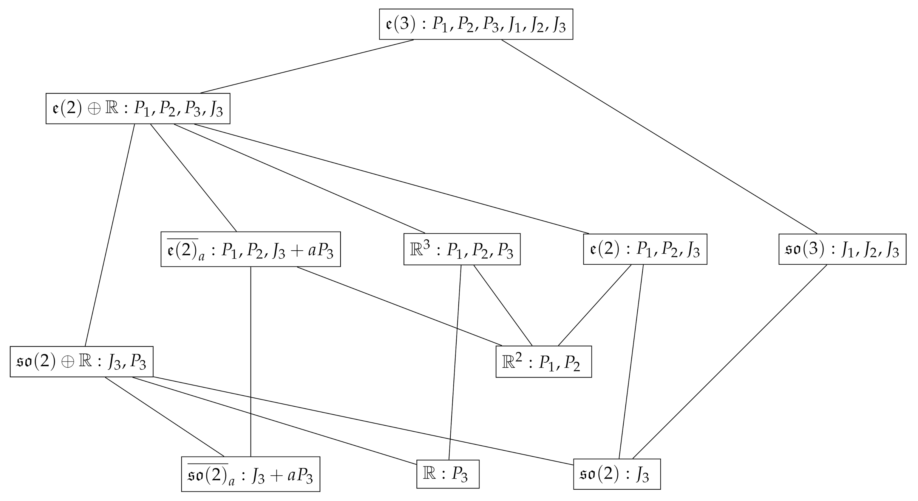
At present time, the classification of all subalgebras of the algebra $\mathfrak{e}\left(3\right)$ up to conjugacy classes of $E\left(3\right)$ is well known (see, for example, [7]); the corresponding Hasse diagram is shown in Figure 1. The diagram is the graph whose vertices correspond to the inequivalent subalgebras in $\mathfrak{e}\left(3\right)$, and the edges indicate the presence of the inclusion relation between the subalgebras.

Let us give some comments on the subalgebras indicated in Figure 1.

The subalgebra $\langle J_3\rangle \simeq \mathfrak{so}\left(2\right)$ generates the group $SO\left(2\right)$ of rotations about the $x_3$-axis, while the subalgebra $\langle P_3\rangle \simeq \mathbb{R}$ corresponds to the subgroup $T^1$ of translations along the same axis. The set of subalgebras $\langle J_3+a{P}_3\rangle \simeq {\overline{\mathfrak{so}\left(2\right)}}_a$ parameterized by the real parameter $a>0$ generates the family of one-dimensional subgroups ${\overline{SO\left(2\right)}}_a$ which are the universal covering groups of $SO\left(2\right)$. The orbits of these subgroups are helices of pitch $2\pi a$.

The subalgebra $\langle P_1,P_2\rangle \simeq {\mathbb{R}}^2$ generates the two-dimensional group $T^2$ of translations in the $x_1{x}_2$-plane. The subalgebra $\langle J_3,P_3\rangle \simeq \mathfrak{so}\left(2\right)\oplus \mathbb{R}$ is associated with the two-dimensional Abelian subgroup in $E\left(3\right)$ whose transformations are rotations about the $x_3$-axis, translations along the same axis, and their combinations.

The three-dimensional algebra $\langle J_1,J_2,J_3\rangle \simeq \mathfrak{so}\left(3\right)$ is the Lie algebra of the rotation group $SO\left(3\right)$, while the Abelian algebra $\langle P_1,P_2,P_3\rangle \simeq {\mathbb{R}}^3$ is the Lie algebra of the translation group $T^3$. The subalgebra $\langle P_1,P_2,J_3\rangle \simeq \mathfrak{e}\left(2\right)$ generates a three-dimensional subgroup in $E\left(3\right)$ which is isomorphic to the isometry group $E\left(2\right)$ of the Euclidean plane. The three-dimensional subgroups ${\overline{E\left(2\right)}}_a$ generated by the family of subalgebras $\langle P_1,P_2,J_3+a{P}_3\rangle \simeq {\overline{\mathfrak{e}\left(2\right)}}_a$ are the universal covering groups of $E\left(2\right)$; all these subgroups act transitively in ${\mathbb{R}}^3$ due to the requirement $a>0$.

The single four-dimensional subalgebra $\langle P_1,P_2,P_3,J_3\rangle \simeq \mathfrak{e}\left(2\right)\oplus \mathbb{R}$ is associated with the subgroup in $E\left(3\right)$ which is the direct product of the translation group $T^3$ and the rotation group $SO\left(2\right)$ about the $x_3$-axis.

There are no five-dimensional subalgebras of the Lie algebra $\mathfrak{e}\left(3\right)$.

For our further purposes, it is necessary to specify a local coordinate system in the Euclidean space ${\mathbb{R}}^3$ and rewrite, in these coordinates, basis Killing vectors ${\xi }_a$ for each subalgebra $\mathcal{G}$ in Figure 1. Due to the fact that we are interested in finding closed 2-forms F such that

$${\mathcal{L}}_{{\xi }_a}F=0,a=1,\dots ,dim\mathcal{G},$$

(15)

it is natural to use a coordinate system in which ${\xi }_a$ have the simplest form. Next, we use four types of local coordinate systems:

(1)

the Cartesian coordinates $(x_1,x_2,x_3)$ for the subalgebras $\mathbb{R}$, ${\mathbb{R}}^2$, ${\mathbb{R}}^3$, $\mathfrak{e}\left(2\right)$, ${\overline{\mathfrak{e}\left(2\right)}}_a$, $\mathfrak{e}\left(2\right)\oplus \mathbb{R}$;

(2)

the cylindrical coordinates $(\rho ,\varphi ,z)$ for the subalgebras $\mathfrak{so}\left(2\right)$ and $\mathfrak{so}\left(2\right)\oplus \mathbb{R}$:

$$\rho ={\left(x_1^2+x_2^2\right)}^{1/2},\varphi =arctan\left(\frac{x_2}{x_1}\right),z=x_3;$$

(3)

the spherical coordinates $(r,\varphi ,\theta )$ for the subalgebra $\mathfrak{so}\left(3\right)$:

$$r={\left(x_1^2+x_2^2+x_3^2\right)}^{1/2},\theta =arccos\left(\frac{x_3}{{\left(x_1^2+x_2^2+x_3^2\right)}^{1/2}}\right),\varphi =arctan\left(\frac{x_2}{x_1}\right);$$

(16)

(4)

the helical coordinates $(\rho ,\varphi ,\zeta )$ for the subalgebra ${\overline{\mathfrak{so}\left(2\right)}}_a$:

$$\rho ={\left(x_1^2+x_2^2\right)}^{1/2},\varphi =arctan\left(\frac{x_2}{x_1}\right),\zeta =x_3+aarctan\left(\frac{x_2}{x_1}\right).$$

(17)

In

Table 1. Inequivalent subalgebras $\mathcal{G}$ of the Lie algebra $\mathfrak{e}\left(3\right)$ and the corresponding electromagnetic fields $(F,\phi )$.

Subalg.	Infinitesimal Generators ${\mathit{X}}_{\mathit{a}}$	Closed 2-Form F Satisfying Equation (15)	Scalar Pot. $\mathit{\phi }$
$\mathbb{R}$	$X_1={\partial }_3$	$f_1(x_1,x_2)d{x}_1\wedge d{x}_2+d{x}_3\wedge d{f}_2(x_1,x_2)$	$f_3(x_1,x_2)$
$\mathfrak{so}\left(2\right)$	$X_1=-{\partial }_{\varphi }$	$f_1(\rho ,z)d\rho \wedge dz+d\varphi \wedge d{f}_2(\rho ,z)$	$f_3(\rho ,z)$
${\overline{\mathfrak{so}\left(2\right)}}_a$	$X_1=-{\partial }_{\varphi }$	$f_1(\rho ,\zeta )d\rho \wedge d\zeta +d\varphi \wedge d{f}_2(\rho ,\zeta )$	$f_3(\rho ,\zeta )$
${\mathbb{R}}^2$	$X_1={\partial }_1,X_2={\partial }_2$	$f_1\left(x_3\right)d{x}_1\wedge d{x}_3+f_2\left(x_3\right)d{x}_2\wedge d{x}_3$	$f_3\left(x_3\right)$
		$\hspace{1em}\hspace{1em}\hspace{1em}\hspace{1em}\hspace{1em}\hspace{1em}\hspace{1em}\hspace{1em}\hspace{1em}\hspace{1em}\hspace{1em}\hspace{1em}\hspace{1em}\hspace{1em}\hspace{1em}+\mu d{x}_1\wedge d{x}_2$
$\mathfrak{so}\left(2\right)\oplus \mathbb{R}$	$X_1=-{\partial }_{\varphi },X_2={\partial }_z$	$f_1\left(\rho \right)d\rho \wedge d\varphi +f_2\left(\rho \right)d\rho \wedge dz$	$f_3\left(\rho \right)$
		$\hspace{1em}\hspace{1em}\hspace{1em}\hspace{1em}\hspace{1em}\hspace{1em}\hspace{1em}\hspace{1em}\hspace{1em}\hspace{1em}\hspace{1em}\hspace{1em}\hspace{1em}\hspace{1em}\hspace{1em}\hspace{1em}\hspace{1em}\hspace{1em}+\mu d\varphi \wedge dz$
${\mathbb{R}}^3$	$X_1={\partial }_1,X_2={\partial }_2,X_3={\partial }_3$	${\mu }_{1}d{x}_1\wedge d{x}_2+{\mu }_{2}d{x}_1\wedge d{x}_3$	0
		$\hspace{1em}\hspace{1em}\hspace{1em}\hspace{1em}\hspace{1em}\hspace{1em}\hspace{1em}\hspace{1em}\hspace{1em}\hspace{1em}\hspace{1em}\hspace{1em}\hspace{1em}\hspace{1em}\hspace{1em}\hspace{1em}\hspace{1em}+{\mu }_{3}d{x}_2\wedge d{x}_3$
$\mathfrak{e}\left(2\right)$	$X_1={\partial }_1,X_2={\partial }_2,$	$\mu d{x}_1\wedge d{x}_2$	$f\left(x_3\right)$
	$X_3=x_2{\partial }_1-x_1{\partial }_2$
${\overline{\mathfrak{e}\left(2\right)}}_a$	$X_1={\partial }_1,X_2={\partial }_2,$	$\left[{\mu }_2\cos \left(\frac{x_3}{a}\right)+{\mu }_3\sin \left(\frac{x_3}{a}\right)\right]d{x}_1\wedge d{x}_3$	0
		$\hspace{1em} \hspace{1em}\hspace{1em}-\left[{\mu }_2\sin \left(\frac{x_3}{a}\right)-{\mu }_3\cos \left(\frac{x_3}{a}\right)\right]d{x}_2\wedge d{x}_3$
	$X_3=x_2{\partial }_1-x_1{\partial }_2+a{\partial }_3$	$\hspace{1em}\hspace{1em}\hspace{1em}\hspace{1em}\hspace{1em}\hspace{1em}\hspace{1em}\hspace{1em}\hspace{1em}\hspace{1em}\hspace{1em}\hspace{1em}+{\mu }_{1}d{x}_1\wedge d{x}_2$
$\mathfrak{so}\left(3\right)$	$X_1=\cos \left(\varphi \right)cot\left(\theta \right){\partial }_{\varphi }+\sin \left(\varphi \right){\partial }_{\theta }$	$\mu \sin \left(\theta \right)d\varphi \wedge d\theta$	$f\left(r\right)$
	$X_2=\sin \left(\varphi \right)cot\left(\theta \right){\partial }_{\varphi }-\cos \left(\varphi \right){\partial }_{\theta }$
	$X_3=-{\partial }_{\varphi }$
$\mathfrak{e}\left(2\right)\oplus \mathbb{R}$	$X_1={\partial }_1,X_2={\partial }_2,X_3={\partial }_3,$	$\mu d{x}_1\wedge d{x}_2$	0
	$X_4=x_2{\partial }_1-x_1{\partial }_2$

, we write out the basis Killing vectors ${\xi }_a$ for each subalgebra $\mathcal{G}$ in the chosen local coordinates (see Figure 1). We also specify the most general forms of closed 2-forms F and scalar potentials $\phi$ (up to addition of an arbitrary constant) satisfying the conditions (15) and (7), respectively. Here, $f,f_1,f_2,f_3$ denote arbitrary smooth functions of their arguments, and $\mu ,{\mu }_1,{\mu }_2,{\mu }_3$ are arbitrary constants.

Remark 4.

As already noted, if two admissible subalgebras $\mathcal{G}$ and ${\mathcal{G}}^{\prime }$ belong to the same conjugacy class in the algebra $\mathfrak{e}\left(3\right)$, then the corresponding classes of electromagnetic fields $\left\{\right(F,\phi \left)\right\}$ and $\left\{(F^{\prime },{\phi }^{\prime })\right\}$ are uniquely transformed into each other by a transformation of the form (14). However, it will be incorrect to say that the electromagnetic fields corresponding to non-conjugate admissible subalgebras are inequivalent. As an example, we point out the electromagnetic fields corresponding to the admissible subalgebras ${\mathbb{R}}^3$ and $\mathfrak{e}\left(2\right)\oplus \mathbb{R}$ in Table 1. These subalgebras are not conjugate in $\mathfrak{e}\left(3\right)$ (since they have different dimensions), but lead to equivalent families of constant electromagnetic fields. This follows from the fact that any constant 2-form in ${\mathbb{R}}^3$ can be reduced to the form $F=\mu d{x}^1\wedge d{x}^2$, $\mu \in \mathbb{R}$, by an orthogonal transformation from $O\left(3\right)$.

Now, we are able to list the possible symmetry algebras $\widehat{\mathcal{G}}$ of time-independent Schrödinger equations in constant electromagnetic fields. To do this, we need to calculate scalar functions ${\chi }_a$ for each Killing vector ${\xi }_a$ in Table 1 (see Equation (10)) and write out the corresponding operators ${\widehat{X}}_a$ according to Formula (11). Below, we list the results of these calculations. For each symmetry algebra $\widehat{\mathcal{G}}$, we also present the matrix $\Vert {\mathbb{F}}_{ab}\Vert$ of the corresponding 2-cocycle (13) and nonzero commutation relations between the constructed symmetry operators. It should be noted that the operators ${\widehat{X}}_a$ have been written out in a gauge-independent form.

3.1. One-Dimensional Subalgebras

3.1.1. Subalgebra $\mathbb{R}\simeq \langle P_3\rangle$

$${\widehat{X}}_0=e,{\widehat{X}}_1={\widehat{p}}_3+e{f}_2(x_1,x_2).$$

3.1.2. Subalgebra $\mathfrak{so}\left(2\right)\simeq \langle J_3\rangle$

$${\widehat{X}}_0=e,{\widehat{X}}_1=-{\widehat{p}}_{\varphi }-e{f}_2(\rho ,z).$$

3.1.3. Subalgebra ${\overline{\mathfrak{so}\left(2\right)}}_a\simeq \langle J_3+a{P}_3\rangle$

$${\widehat{X}}_0=e,{\widehat{X}}_1=-{\widehat{p}}_{\varphi }-e{f}_2(\rho ,\zeta ).$$

In all these cases, the symmetry algebra $\widehat{\mathcal{G}}=\langle {\widehat{X}}_0,{\widehat{X}}_1\rangle$ is isomorphic to a trivial one-dimensional extension of the one-dimensional Abelian Lie algebra $\mathbb{R}$.

3.2. Two-Dimensional Subalgebras

3.2.1. Subalgebra ${\mathbb{R}}^2\simeq \langle P_1,P_2\rangle$

$${\widehat{X}}_0=e,$$

$${\widehat{X}}_1={\widehat{p}}_1-e\mu x_2-e\int f_1\left(x_3\right)d{x}_3,{\widehat{X}}_2={\widehat{p}}_2+e\mu x_1-e\int f_2\left(x_3\right)d{x}_3,$$

$$\Vert {\mathbb{F}}_{ab}\Vert =\left(\begin{array}{cc}0& \mu \\ -\mu & 0\end{array}\right);$$

$$[{\widehat{X}}_1,{\widehat{X}}_2]=-i\mu {\widehat{X}}_0.$$

The symmetry algebra $\widehat{\mathcal{G}}=\langle {\widehat{X}}_0,{\widehat{X}}_1,{\widehat{X}}_2\rangle$ is a one-dimensional central extension of the two-dimensional Abelian Lie algebra ${\mathbb{R}}^2$. This extension is nontrivial for $\mu \ne 0$.

3.2.2. Subalgebra $\mathfrak{so}\left(2\right)\oplus \mathbb{R}\simeq \langle J_3,P_3\rangle$

$${\widehat{X}}_0=e,$$

$${\widehat{X}}_1=-{\widehat{p}}_{\varphi }+e\mu z-e\int f_1\left(\rho \right)d\rho ,{\widehat{X}}_2={\widehat{p}}_z+e\mu \varphi +e\int f_2\left(\rho \right)d\rho ,$$

$$\Vert {\mathbb{F}}_{ab}\Vert =\left(\begin{array}{cc}0& -\mu \\ \mu & 0\end{array}\right);$$

$$[{\widehat{X}}_1,{\widehat{X}}_2]=i\mu {\widehat{X}}_0.$$

The symmetry algebra $\widehat{\mathcal{G}}=\langle {\widehat{X}}_0,{\widehat{X}}_1,{\widehat{X}}_2\rangle$ is a one-dimensional central extension of the two-dimensional Abelian Lie algebra $\mathfrak{so}\left(2\right)\oplus \mathbb{R}$. This extension is nontrivial for $\mu \ne 0$.

3.3. Three-Dimensional Subalgebras

3.3.1. Subalgebra ${\mathbb{R}}^3\simeq \langle P_1,P_2,P_3\rangle$

$${\widehat{X}}_0=e,$$

$${\widehat{X}}_1={\widehat{p}}_1-e\left({\mu }_1{x}_2+{\mu }_2{x}_3\right),{\widehat{X}}_2={\widehat{p}}_2+e\left({\mu }_1{x}_1-{\mu }_3{x}_3\right),{\widehat{X}}_3={\widehat{p}}_3+e\left({\mu }_2{x}_1+{\mu }_3{x}_2\right),$$

$$\Vert {\mathbb{F}}_{ab}\Vert =\left(\begin{array}{ccc}0& {\mu }_1& {\mu }_2\\ -{\mu }_1& 0& {\mu }_3\\ -{\mu }_2& -{\mu }_3& 0\end{array}\right);$$

$$[{\widehat{X}}_1,{\widehat{X}}_2]=-i{\mu }_1{\widehat{X}}_0,[{\widehat{X}}_1,{\widehat{X}}_3]=-i{\mu }_2{\widehat{X}}_0,[{\widehat{X}}_2,{\widehat{X}}_3]=-i{\mu }_3{\widehat{X}}_0.$$

The symmetry algebra $\widehat{\mathcal{G}}=\langle {\widehat{X}}_0,{\widehat{X}}_1,{\widehat{X}}_2,{\widehat{X}}_3\rangle$ is a one-dimensional central extension of the three-dimensional Abelian Lie algebra ${\mathbb{R}}^3$. This extension is nontrivial for ${\mu }_1^2+{\mu }_2^2+{\mu }_3^2\ne 0$.

3.3.2. Subalgebra $\mathfrak{e}\left(2\right)\simeq \langle P_1,P_2,J_3\rangle$

$${\widehat{X}}_0=e,$$

(18)

$${\widehat{X}}_1={\widehat{p}}_1-e\mu x_2,{\widehat{X}}_2={\widehat{p}}_2+e\mu x_1,{\widehat{X}}_3=x_2{\widehat{p}}_1-x_1{\widehat{p}}_2-\frac{1}{2}e\mu \left(x_1^2+x_2^2\right),$$

(19)

$$\Vert {\mathbb{F}}_{ab}\Vert =\left(\begin{array}{ccc}0& \mu & 0\\ -\mu & 0& 0\\ 0& 0& 0\end{array}\right);$$

$$[{\widehat{X}}_1,{\widehat{X}}_2]=-i\mu {\widehat{X}}_0,[{\widehat{X}}_1,{\widehat{X}}_3]=i{\widehat{X}}_2,[{\widehat{X}}_2,{\widehat{X}}_3]=-i{\widehat{X}}_1.$$

The symmetry algebra $\widehat{\mathcal{G}}=\langle {\widehat{X}}_0,{\widehat{X}}_1,{\widehat{X}}_2,{\widehat{X}}_3\rangle$ is a one-dimensional central extension of the three-dimensional Lie algebra $\mathfrak{e}\left(2\right)$. This extension is nontrivial for $\mu \ne 0$.

3.3.3. Subalgebra ${\overline{\mathfrak{e}\left(2\right)}}_a\simeq \langle P_1,P_2,J_3+a{P}_3\rangle$

$${\widehat{X}}_0=e,$$

(20)

$${\widehat{X}}_1={\widehat{p}}_1+ea\left[{\mu }_3\cos \left(\frac{x_3}{a}\right)-{\mu }_2\sin \left(\frac{x_3}{a}\right)\right]-e{\mu }_1{x}_2,$$

(21)

$${\widehat{X}}_2={\widehat{p}}_2-ea\left[{\mu }_2\cos \left(\frac{x_3}{a}\right)+{\mu }_3\sin \left(\frac{x_3}{a}\right)\right]+e{\mu }_1{x}_1,$$

(22)

$$\begin{array}{c}{\widehat{X}}_3=x_2{\widehat{p}}_1-x_1{\widehat{p}}_2+a{\widehat{p}}_3+\hfill \\ \hspace{1em}\hspace{1em}\hspace{1em}\hspace{1em}ea\left[({\mu }_2{x}_1+{\mu }_3{x}_2)\cos \left(\frac{x_3}{a}\right)+({\mu }_3{x}_1-{\mu }_2{x}_2)\sin \left(\frac{x_3}{a}\right)\right]-\frac{1}{2}e{\mu }_1\left(x_1^2+x_2^2\right),\hfill \end{array}$$

(23)

$$\Vert {\mathbb{F}}_{ab}\Vert =\left(\begin{array}{ccc}0& {\mu }_1& 0\\ -{\mu }_1& 0& 0\\ 0& 0& 0\end{array}\right);$$

$$[{\widehat{X}}_1,{\widehat{X}}_2]=-i{\mu }_1{\widehat{X}}_0,[{\widehat{X}}_1,{\widehat{X}}_3]=i{\widehat{X}}_2,[{\widehat{X}}_2,{\widehat{X}}_3]=-i{\widehat{X}}_1.$$

The symmetry algebra $\widehat{\mathcal{G}}=\langle {\widehat{X}}_0,{\widehat{X}}_1,{\widehat{X}}_2,{\widehat{X}}_3\rangle$ is a one-dimensional central extension of the three-dimensional Lie algebra ${\overline{\mathfrak{e}\left(2\right)}}_a$. This extension is nontrivial for ${\mu }_1\ne 0$.

3.3.4. Subalgebra $\mathfrak{so}\left(3\right)\simeq \langle J_1,J_2,J_3\rangle$

$${\widehat{X}}_0=e,$$

(24)

$${\widehat{X}}_1=\cos \left(\varphi \right)cot\left(\theta \right){\widehat{p}}_{\varphi }+\sin \left(\varphi \right){\widehat{p}}_{\theta }-e\mu \sin \left(\theta \right)\cos \left(\varphi \right),$$

(25)

$${\widehat{X}}_2=\sin \left(\varphi \right)cot\left(\theta \right){\widehat{p}}_{\varphi }-\cos \left(\varphi \right){\widehat{p}}_{\theta }-e\mu \sin \left(\theta \right)\sin \left(\varphi \right),$$

(26)

$${\widehat{X}}_3=-{\widehat{p}}_{\varphi }-e\mu \cos \left(\theta \right),$$

(27)

$$\Vert {\mathbb{F}}_{ab}\Vert =\left(\begin{array}{ccc}0& 0& 0\\ 0& 0& 0\\ 0& 0& 0\end{array}\right);$$

$$[{\widehat{X}}_1,{\widehat{X}}_2]=-i{\widehat{X}}_3,[{\widehat{X}}_1,{\widehat{X}}_3]=i{\widehat{X}}_2,[{\widehat{X}}_2,{\widehat{X}}_3]=-i{\widehat{X}}_1.$$

The symmetry algebra $\widehat{\mathcal{G}}=\langle {\widehat{X}}_0,{\widehat{X}}_1,{\widehat{X}}_2,{\widehat{X}}_3\rangle$ is a trivial one-dimensional central extension of the three-dimensional Lie algebra $\mathfrak{so}\left(3\right)$ for any values of the constant $\mu$.

3.4. Four-Dimensional Subalgebras

Subalgebra $\mathfrak{e}\left(2\right)\oplus \mathbb{R}\simeq \langle P_1,P_2,P_3,J_3\rangle$

$${\widehat{X}}_0=e,$$

(28)

$${\widehat{X}}_1={\widehat{p}}_1-e\mu x_2,{\widehat{X}}_2={\widehat{p}}_2+e\mu x_1,{\widehat{X}}_3={\widehat{p}}_3,{\widehat{X}}_4=x_2{\widehat{p}}_1-x_1{\widehat{p}}_2-\frac{1}{2}e\mu \left(x_1^2+x_2^2\right).$$

(29)

$$\Vert {\mathbb{F}}_{ab}\Vert =\left(\begin{array}{cccc}0& \mu & 0& 0\\ -\mu & 0& 0& 0\\ 0& 0& 0& 0\\ 0& 0& 0& 0\end{array}\right);$$

$$[{\widehat{X}}_1,{\widehat{X}}_2]=-i\mu {\widehat{X}}_0,[{\widehat{X}}_1,{\widehat{X}}_4]=i{\widehat{X}}_2,[{\widehat{X}}_2,{\widehat{X}}_4]=-i{\widehat{X}}_1.$$

The symmetry algebra $\widehat{\mathcal{G}}=\langle {\widehat{X}}_0,{\widehat{X}}_1,{\widehat{X}}_2,{\widehat{X}}_3,{\widehat{X}}_4\rangle$ is a one-dimensional central extension of the four-dimensional Lie algebra $\mathfrak{e}\left(2\right)\oplus \mathbb{R}$. This extension is nontrivial for $\mu \ne 0$.

4. Noncommutative Integration of the Schrödinger Equation

Let us show how to make use of the symmetry algebra $\widehat{\mathcal{G}}$ to construct exact solutions of the Schrödinger equation (1).

Traditionally, to solve this problem, one uses the well-known method of separation of variables. For the applicability of this method, one assumes that the Hamiltonian $\widehat{H}$ belongs to a three-dimensional commutative algebra of first- or second-order symmetry operators ${\widehat{Y}}_{\alpha }$ [14]. In this case, a basis of solutions to the Schrödinger equation can be found from the eigenvalue problem

$${\widehat{Y}}_{\alpha }\psi =J_{\alpha }\psi ,\alpha =1,2,3,$$

(30)

where ${\widehat{Y}}_1=\widehat{H}$, $J_1=E$ and $[{\widehat{Y}}_{\alpha },{\widehat{Y}}_{\beta }]=0$ for all $\alpha ,\beta =1,2,3$. The basic difficulty here is that the algebra $\widehat{\mathcal{G}}$ is, in general, noncommutative, and there is no guarantee that it contains two-dimensional commutative subalgebras, which, together with the Hamiltonian, can be used to solve the eigenvalue problem (30). In practice, this difficulty is overcome by the extension of the symmetry algebra $\widehat{\mathcal{G}}$ to the universal enveloping algebra $U\left(\widehat{\mathcal{G}}\right)$, in which a pair of second-order commuting operators is sought.

There is, however, an alternative way to construct exact solutions of the Schrödinger Equation (1), which does not involve the use of higher-order symmetry operators and deals only with the original noncommutative symmetry algebra $\widehat{\mathcal{G}}$. This is the so-called noncommutative integration method of linear PDEs [16,17,18] developed by Shapovalov and Shirokov by analogy with the noncommutative integration method of finite-dimensional Hamiltonian systems [25]. This section aims to demonstrate this method as a basis for a unified and effective approach to constructing exact solutions of time-independent Schrödinger equations with nontrivial symmetry algebras.

Before proceeding further, let us clarify what we mean by the “integrability” of the Schrödinger equation.

Definition 1.

The Schrödinger equation (Equation (1)) is called integrable if constructing a basis of its solution space is reduced to solving systems of ordinary differential equations and using quadratures.

Remark 5.

In quantum mechanics, the term “basis” commonly refers to a certain Hilbert space of global solutions of the Schrödinger equation. The construction of such global solutions proceeds by “gluing” local ones and requires an analysis of the additional topological properties of the corresponding underlying manifold. However, within the framework of our approach, we will not consider the global aspect and the term “basis” will be used only in the following local sense. By a basis of the solution space of the Schrödinger Equation (1), we will mean a parametric family of particular solutions ${\psi }_J(x,q)$ with the property of local completeness in the sense that a formal expansion of the general solution can be constructed using ${\psi }_J(x,q)$.

Let us suppose that Equation (1) admits an $(n+1)$-dimensional symmetry algebra $\widehat{\mathcal{G}}$ with the basis

$${\widehat{X}}_0=e,{\widehat{X}}_1={\xi }_1^i\left(x\right){\widehat{p}}_i+e{\chi }_1\left(x\right),\dots ,{\widehat{X}}_n={\xi }_n^i\left(x\right){\widehat{p}}_i+e{\chi }_n\left(x\right).$$

(31)

We have shown in Section 2 that this algebra is isomorphic to a one-dimensional central extension of an n-dimensional Lie algebra $\mathcal{G}$ of admissible Killing vectors ${\xi }_a={\xi }_a^i\left(x\right){\partial }_i$.

We consider a family of operator-irreducible representations of the Lie algebra $\widehat{\mathcal{G}}$ parameterized by real parameters $J=(J_1,\dots ,J_s)$ and realized by the first-order differential operators ${\widehat{\ell }}_a(q,{\partial }_q;J)$ acting on a space of functions on variables $q=(q^1,\dots ,q^m)$ [26]:

$${\widehat{\ell }}_0=-e,{\widehat{\ell }}_a(q,{\partial }_q;J)={\zeta }_a^{\gamma }\left(q\right)\frac{\partial }{\partial q^{\gamma }}+{\vartheta }_a(q;J),a=1,\dots ,dim\mathcal{G},$$

(32)

$$[{\widehat{\ell }}_a,{\widehat{\ell }}_b]=-i\left(C_{ab}^c{\widehat{\ell }}_c-e{\mathbb{F}}_{ab}\right).$$

Here, $C_{ab}^c$ are the structure constants of the admissible Lie subalgebra $\mathcal{G}$, ${\mathbb{F}}_{ab}$ are components of its 2-cocycle, which is defined by an electromagnetic field from Formula (13). Moreover, $s={\mathrm{ind}}_{\mathbb{F}}\mathcal{G}$ and $m=\frac{1}{2}\left(dim\mathcal{G}-{\mathrm{ind}}_{\mathbb{F}}\mathcal{G}\right)$, where the nonnegative integer ${\mathrm{ind}}_{\mathbb{F}}\mathcal{G}$ is called the cohomological index of the admissible Lie algebra $\mathcal{G}$ [19,27]:

$${\mathrm{ind}}_{\mathbb{F}}\mathcal{G}\equiv dim\mathcal{G}-\underset{f\in {\mathcal{G}}^{*}}{sup}\mathrm{rank}\Vert {\mathbb{F}}_{ab}+C_{ab}^c{f}_c\Vert .$$

(33)

Due to the operator-irreducibility of the representation (32), any Casimir operator of $\widehat{\mathcal{G}}$ is a multiple of the unit operator:

$$K\left(\widehat{\ell }(q,{\partial }_q;J)\right)=\kappa \left(J\right)·\mathrm{id}.$$

(34)

The quantities $J_{\mu }$, which parameterize the operators ${\widehat{\ell }}_a(q,{\partial }_q;J)$, can take both continuous and discrete values. It follows from the equality (34) that they, in fact, parameterize a spectrum of Casimir operators of the algebra $\widehat{\mathcal{G}}$.

The operator-irreducible representation of the Lie algebra $\widehat{\mathcal{G}}$ satisfying the above conditions is called the λ-representation of the algebra $\widehat{\mathcal{G}}$. As we will see, it plays a key role in the noncommutative integration method of the Schrödinger Equation (1). It is important to note that the problem of constructing $\lambda$-representations of Lie algebras is directly related to the structure of coadjoint orbits of the corresponding Lie groups and, in each particular case, can be constructively solved by methods of linear algebra (see, for example, [18,20,26]).

Let us now describe a method for reducing the number of independent variables in Schrödinger equations by using symmetry algebras $\widehat{\mathcal{G}}$. We consider the linear system of first-order equations

$${\widehat{X}}_a(x,{\partial }_x){\psi }_J(x,q)=-{\widehat{\ell }}_a(q,{\partial }_q;J){\psi }_J(x,q),a=1,\dots ,dim\mathcal{G},$$

(35)

where ${\widehat{X}}_a(x,{\partial }_x)$ are the basis non-trivial operators from $\widehat{\mathcal{G}}$ and ${\widehat{\ell }}_a(q,{\partial }_q;J)$ are the corresponding operators of $\lambda$-representation for this algebra. The unknown complex-valued function ${\psi }_J(x,q)$ is a function of the variables x and q, which depends on the quantities J as on parameters.

It is not difficult to verify that the system (35) is compatible since the sets of operators $\left\{{\widehat{X}}_a\right\}$ and $\left\{{\widehat{\ell }}_a\right\}$ form representations of the same Lie algebra. Because (35) is the first-order system of partial differential equations, it can be easily integrated using quadratures, for example, by the method of characteristics. The corresponding general solution can always be written in the form

$${\psi }_J(x,q)={\Phi }_J\left(u(x,q)\right)e^{i{R}_J(x,q)},$$

(36)

where $R_J(x,q)$ is a function determined by the system of Equation (35), ${\Phi }_J$ is an arbitrary function, $u(x,q)=(u^1(x,q),\dots ,u^k(x,q))$ are functionally independent first integrals of the corresponding homogeneous system.

We substitute the general solution (36) into the Schrödinger equation (1):

$$\widehat{H}{\psi }_J(x,q)=E{\psi }_J(x,q).$$

(37)

Since the operators ${\widehat{X}}_a$ commute with $\widehat{H}$, the solution space of the system (35) is invariant under the Hamiltonian. This means that the action of $\widehat{H}$ on ${\psi }_J(x,q)$ can be written as

$$\widehat{H}{\psi }_J(x,q)=\widehat{H}\left({\Phi }_J\left(u(x,q)\right)e^{i{R}_J(x,q)}\right)={\tilde{\Phi }}_J\left(u(x,q)\right)e^{i{R}_J(x,q)},$$

(38)

where ${\tilde{\Phi }}_J$ is a new function on the characteristics $u(x,q)$. Defining a linear operator ${\widehat{h}}_J$ by

$${\widehat{h}}_J{\Phi }_J\equiv e^{-i{R}_J}\widehat{H}{\Phi }_J{e}^{i{R}_J},$$

we have ${\tilde{\Phi }}_J={\widehat{h}}_J{\Phi }_J$ and hence Equation (37) is reduced to the linear partial differential equation

$${\widehat{h}}_J{\Phi }_J=E{\Phi }_J,$$

(39)

which is called the reduced Schrödinger equation.

It is easy to see that the operator ${\widehat{h}}_J$, as well as the Hamiltonian $\widehat{H}$, is the second-order differential operator; it acts on functions of k variables $u(x,q)=(u^1(x,q),\dots ,u^k(x,q))$ considered now as independent. Thus, we have shown that the function (36) satisfies the Schrödinger Equation (1) if and only if the function ${\Phi }_J$ is a solution of the reduced Schrödinger Equation (39). The quantities q and J can be regarded as a set of “quantum numbers”, which together with E parameterize the constructed family of solutions.

Let us calculate the number k of the functionally independent first integrals of the system (35), which is equal to the number of independent variables in the reduced Schrödinger equation. For this, we note that the first integrals are functions $u(x,q)$ satisfying the homogeneous system of differential equations

$${\xi }_a^i\left(x\right)\frac{\partial u(x,q)}{\partial x^i}+{\zeta }_a^{\gamma }\left(q\right)\frac{\partial u(x,q)}{\partial q^{\gamma }}=0,a=1,\dots ,n=dim\mathcal{G},$$

(40)

where ${\xi }_a^i\left(x\right)$ are the components of basis admissible Killing vectors, ${\zeta }_a^{\gamma }\left(q\right)$ are the coefficients of derivatives $\partial /\partial q^{\gamma }$ in $\lambda$-representation operators of the symmetry algebra $\widehat{\mathcal{G}}$ (see Equation (32)). In order to avoid several technical complications, we assume that there are no identities for Killing vectors ${\xi }_a$ from the admissible subalgebra, that is, nontrivial relations of the form $c^{a_1{a}_2\dots a_l}{\xi }_{a_1}^{i_1}\left(x\right){\xi }_{a_2}^{i_2}\left(x\right)\dots {\xi }_{a_l}^{i_l}\left(x\right)\equiv 0$, where $c^{a_1{a}_2\dots a_l}$ are constants. (Only such cases arise in this study.) Then, we can claim that the number of functionally independent solutions of the homogeneous system (40) is equal to

$$k=3+\frac{1}{2}\left(dim\mathcal{G}-{\mathrm{ind}}_{\mathbb{F}}\mathcal{G}\right)-dim\mathcal{G}=3-\frac{1}{2}\left(dim\mathcal{G}+{\mathrm{ind}}_{\mathbb{F}}\mathcal{G}\right).$$

(Recall that the number of variables q is equal to $m=\frac{1}{2}\left(dim\mathcal{G}-{\mathrm{ind}}_{\mathbb{F}}\mathcal{G}\right)$.) In particular, the reduced Schrödinger equation is an ordinary differential (or algebraic) equation in the case of $k\le 1$ that leads to the condition

$$dim\mathcal{G}+{\mathrm{ind}}_{\mathbb{F}}\mathcal{G}\ge 4.$$

(41)

Thus, if the corresponding admissible subalgebra $\mathcal{G}$ and its 2-cocycle (13) satisfy the condition (41), then the Schrödinger equation (1) is integrable in the sense of Definition 1.

In Section 3, we have listed all time-independent electromagnetic fields for which the corresponding Schrödinger equations admit nontrivial symmetry algebras. As shown above, the equivalence classes of such fields are given by inequivalent subalgebras of the Lie algebra $\mathfrak{e}\left(3\right)$; the latter are just the possible admissible subalgebras. Now, using the condition (41), we can select among the admissible subalgebras $\mathcal{G}\subset \mathfrak{e}\left(3\right)$ those for which the Schrödinger equation can be solved by the noncommutative integration method. The results of this classification are shown in

Table 2. Integrable cases of the Schrödinger equation.

Subalgebra	$dim\mathcal{G}$	${\mathbf{ind}}_{\mathbb{F}}\mathcal{G}$	k	Integrability
$\mathbb{R}$	1	1	2	No
$\mathfrak{so}\left(2\right)$	1	1	2	No
${\overline{\mathfrak{so}\left(2\right)}}_a$, $a>0$	1	1	2	No
${\mathbb{R}}^2$	2	0, if $\mu \ne 0$	2	No
		2, if $\mu =0$	1	Yes
$\mathfrak{so}\left(2\right)\oplus \mathbb{R}$	2	0, if $\mu \ne 0$	2	No
		2, if $\mu =0$	1	Yes
${\mathbb{R}}^3$	3	1, if $\sum {\mu }_i^2\ne 0$	1	Yes
		3, if $\sum {\mu }_i^2=0$	0
$\mathfrak{e}\left(2\right)$	3	1	1	Yes
${\overline{\mathfrak{e}\left(2\right)}}_a$	3	1	1	Yes
$\mathfrak{so}\left(3\right)$	3	1	1	Yes
$\mathfrak{e}\left(2\right)\oplus \mathbb{R}$	4	1	0	Yes

, where for each subalgebra $\mathcal{G}$, we indicate its dimension $dim\mathcal{G}$, cohomological index ${\mathrm{ind}}_{\mathbb{F}}\mathcal{G}$, number of independent variables q in a reduced equation which is equal to $k=3-\left(dim\mathcal{G}+{\mathrm{ind}}_{\mathbb{F}}\mathcal{G}\right)/2$ and, finally, indicate whether the Schrödinger equation with the corresponding symmetry algebra $\widehat{\mathcal{G}}$ is integrable or not.

Remark 6.

Of course, there exist integrable cases of the time-independent Schrödinger equation that are not covered by condition (41). In particular, this happens in the case when there are the so-called “hidden” symmetries of Equation (1) associated with higher-order symmetry operators, which do not belong to the universal enveloping algebra $U\left(\widehat{\mathcal{G}}\right)$. However, we are not considering such cases here.

4.1. Reduction of Schrödinger Equations to Ordinary Differential Equations

Let us demonstrate how the noncommutative integration method allows one to reduce Schrödinger equations in electromagnetic fields with the admissible subalgebras $\mathfrak{e}\left(2\right)$, ${\overline{\mathfrak{e}\left(2\right)}}_a$, $\mathfrak{so}\left(3\right)$, and $\mathfrak{e}\left(2\right)\oplus \mathbb{R}$ to ordinary differential equations. We do not consider here the integrable cases with the subalgebras ${\mathbb{R}}^2$ and $\mathfrak{so}\left(2\right)\oplus \mathbb{R}$ ($\mu =0$) as trivial; for both of these situations, it is easy to reduce the original Schrödinger equation to an ordinary differential equation using a pair of commuting first-order symmetry operators. Below, we also do not discuss the case of the admissible subalgebra ${\mathbb{R}}^3$ because the corresponding class of electromagnetic fields is equivalent to a class of fields with the admissible subalgebra $\mathfrak{e}\left(2\right)\oplus \mathbb{R}$ (see Remark 4).

4.1.1. Case $\mathfrak{e}\left(2\right)$

In the Cartesian coordinates, the basis vector fields of the admissible subalgebra $\mathfrak{e}\left(2\right)$ are written as

$${\xi }_1=\frac{\partial }{\partial x_1},{\xi }_2=\frac{\partial }{\partial x_2},{\xi }_3=x_2\frac{\partial }{\partial x_1}-x_1\frac{\partial }{\partial x_2}.$$

The class of electromagnetic fields determined by this subalgebra is given by the magnetic 2-form F and the scalar potential $\phi$ of the form (see Table 1):

$$F=\mu d{x}_1\wedge d{x}_2,\phi =f\left(x_3\right),$$

where $\mu$ is a constant, $f\left(x_3\right)$ is an arbitrary function depending only on the $x_3$-coordinate. Thus, the electric and magnetic components of this field are directed along the $O{x}_3$-axis; the magnetic field is uniform, but the electric field generally depends on the $x_3$-coordinate.

Choosing the magnetic field potential in the form $A=\mu \left(-x_{2}d{x}_1+x_{1}d{x}_2\right)/2$, we obtain the corresponding Schrödinger equation

$$-\frac{1}{2m}\Delta \psi +\frac{ie\mu }{2m}\left(x_1\frac{\partial \psi }{\partial x_2}-x_2\frac{\partial \psi }{\partial x_1}\right)+\frac{e^2{\mu }^2}{8m}\left(x_1^2+x_2^2\right)\psi +ef\left(x_3\right)\psi =E\psi ,$$

(42)

where $\Delta ={\partial }_1^2+{\partial }_2^2+{\partial }_3^2$ is the Laplace operator. The symmetry algebra $\widehat{\mathcal{G}}$ of this equation is generated by the operators (18) and (19); for the chosen gauge, these are written in the form

$${\widehat{X}}_0=e,{\widehat{X}}_1=-i\frac{\partial }{\partial x_1}-\frac{1}{2}e\mu x_2,{\widehat{X}}_2=-i\frac{\partial }{\partial x_2}+\frac{1}{2}e\mu x_1,{\widehat{X}}_3=-i\left(x_2\frac{\partial }{\partial x_1}-x_1\frac{\partial }{\partial x_2}\right).$$

(43)

Let us realize the Lie algebra $\widehat{\mathcal{G}}$ by the $\lambda$-representation operators ${\widehat{\ell }}_a(q,{\partial }_q;J)$ acting in the space of holomorphic functions of complex variable $q\in \mathbb{C}$ and parameterized by the continuous real parameter $J\in (-\infty ,+\infty )$:

$${\widehat{\ell }}_0=-e,{\widehat{\ell }}_1=\frac{1}{2}\frac{\partial }{\partial q}-e\mu q,{\widehat{\ell }}_2=\frac{i}{2}\frac{\partial }{\partial q}+ie\mu q,{\widehat{\ell }}_3=-q\frac{\partial }{\partial q}+J;$$

(44)

$$[{\widehat{\ell }}_1,{\widehat{\ell }}_2]=-i\mu {\widehat{\ell }}_0,[{\widehat{\ell }}_1,{\widehat{\ell }}_2]=i{\widehat{\ell }}_2,[{\widehat{\ell }}_2,{\widehat{\ell }}_3]=-i{\widehat{\ell }}_3,$$

The corresponding Casimir operator is

$$K\left(\widehat{\ell }\right)={\widehat{\ell }}_1^2+{\widehat{\ell }}_2^2-2\mu e{\widehat{\ell }}_3=-e\mu \left(2J+1\right).$$

Solving the first-order linear system (35), we easily find its general solution

$${\psi }_J(x_1,x_2,x_3;q)={\Phi }_J\left(u\right){\left[x_1+i\left(x_2+2q\right)\right]}^{J}exp\left[\frac{e\mu (x_1^2+x_2^2)}{4}+e\mu q(i{x}_1+x_2)\right],$$

(45)

where $u=x_3$, ${\Phi }_J\left(u\right)$ is an arbitrary function of its argument. This solution is not a single-valued function of coordinates. Indeed, if we let $q=0$ and $x+iy=\rho e^{i\phi }$, we obtain the expression

$${\psi }_J(\rho \cos \phi ,\rho \sin \phi ,x_3,0)={\Phi }_J\left(x_3\right){\rho }^J{e}^{iJ\phi }exp\left(\frac{e\mu {\rho }^2}{4}\right),$$

which, generally speaking, is not a single-valued function due to the multiplier $e^{iJ\phi }$. The requirement that this function is single-valued leads to the “quantization condition” according to that the parameter J must be an integer.

Substituting the function (45) into Equation (42), we come, after simple transformations, to the reduced Schrödinger equation (Equation (39)):

$${\widehat{h}}_J{\Phi }_J\left(u\right)\equiv \left[-\frac{1}{2m}\frac{d^2}{d{u}^2}-\frac{e\mu }{2m}\left(2J+1\right)+ef\left(u\right)\right]{\Phi }_J\left(u\right)=E{\Phi }_J\left(u\right),$$

(46)

Thus, the original Equation (42) is reduced to a one-dimensional Schrödinger equation with the effective potential:

$$V_J\left(u\right)=e\left[f\left(u\right)-\frac{e\mu }{2m}\left(2J+1\right)\right].$$

Due to the arbitrariness of the function $f\left(u\right)$, the solutions of the ordinary differential equation (46) are not expressed in terms of known special functions in the general case.

4.1.2. Case ${\overline{\mathfrak{e}\left(2\right)}}_a$

Let us transform the Cartesian coordinates $(x^1,x^2,x^3)$ to the helical coordinates$(\rho ,\varphi ,\zeta )$ (see Equation (17)). The basis vector fields ${\xi }_a\in {\overline{\mathfrak{e}\left(2\right)}}_a$ in these coordinates have the form

$${\xi }_1=\cos \left(\varphi \right)\frac{\partial }{\partial \rho }-\frac{\sin \left(\varphi \right)}{\rho }\left(\frac{\partial }{\partial \varphi }+a\frac{\partial }{\partial \zeta }\right),{\xi }_2=\sin \left(\varphi \right)\frac{\partial }{\partial \rho }+\frac{\cos \left(\varphi \right)}{\rho }\left(\frac{\partial }{\partial \varphi }+a\frac{\partial }{\partial \zeta }\right),{\xi }_3=-\frac{\partial }{\partial \varphi }.$$

The corresponding class of electromagnetic fields is determined by the closed 2-form

$$\begin{array}{c}F={\mu }_1\rho d\rho \wedge d\varphi +a\left[{\mu }_2\cos \left(\frac{\zeta }{a}\right)-{\mu }_3\sin \left(\frac{\zeta }{a}\right)\right]d\rho \wedge d\varphi +\hfill \\ \hspace{1em}\hspace{1em}\hspace{1em}\hspace{1em}\hspace{1em}\hspace{1em}\hspace{1em}+\left[{\mu }_2\cos \left(\frac{\zeta }{a}\right)+{\mu }_3\sin \left(\frac{\zeta }{a}\right)\right]d\rho \wedge d\zeta -\rho \left[{\mu }_2\sin \left(\frac{\zeta }{a}\right)-{\mu }_3\cos \left(\frac{\zeta }{a}\right)\right]d\varphi \wedge d\zeta ,\hfill \end{array}$$

and the scalar potential $\phi =0$ (see Table 1), where ${\mu }_1$, ${\mu }_2$, ${\mu }_3$ are arbitrary constants, $a>0$. We introduce the notation

$${\mu }_1=\mu ,{\mu }_2=B_0\cos \theta ,{\mu }_3=B_0\sin \theta ,$$

where $\mu$, $B_0$ and $\theta$ are new constants; moreover, $B_0>0$, $0\le \theta <2\pi$. By rotations in the $x^1{x}^2$-plane, we can achieve that $\theta =0$ (we recall that hlthe electromagnetic fields up to the equivalence relation (14) are considered). Thus, we will actually study a class of magnetic fields of the form

$$F=\mu \rho d\rho \wedge d\varphi +B_0\left[\cos \left(\frac{\zeta }{a}\right)d\rho \wedge \left(d\zeta -ad\varphi \right)-\rho \sin \left(\frac{\zeta }{a}\right)d\varphi \wedge d\zeta \right].$$

It is easy to see that this magnetic field is a superposition of a uniform magnetic field directed along the $x_3$-axis and a magnetic field whose direction is everywhere parallel to the current density vector (the so-called force-free field).

Let us choose the magnetic field potential in the following form

$$A=\frac{\mu {\rho }^2}{2}d\varphi +B_0\rho \cos \left(\frac{\zeta }{a}\right)(d\zeta -ad\varphi ).$$

(47)

In this gauge fixing, the Schrödinger Equation (1) is written as

$$\begin{array}{c}-\frac{1}{2m}\Delta \psi +\frac{ie\mu }{2m}\frac{\partial \psi }{\partial \varphi }+\frac{ie}{2m}\left[a\mu +2B_0\rho \cos \left(\frac{\zeta }{a}\right)\right]\frac{\partial \psi }{\partial \zeta }\hfill \\ \hspace{1em}\hspace{1em}\hspace{1em}\hspace{1em}\hspace{1em}\hspace{1em}\hspace{1em}\hspace{1em}\hspace{1em}\hspace{1em}\hspace{1em}\hspace{1em}\hspace{1em}\hspace{1em}+\frac{e\rho }{2ma}\left[ea{B}_0^2\rho {\cos }^2\left(\frac{\zeta }{a}\right)-i{B}_0\sin \left(\frac{\zeta }{a}\right)+\frac{ea{\mu }^2\rho }{4}\right]\psi =E\psi ,\hfill \end{array}$$

(48)

where $\Delta$ is the Laplace operator in the helical coordinates (17):

$$\Delta =\frac{1}{\rho }\frac{\partial }{\partial \rho }\left(\rho \frac{\partial }{\partial \rho }\right)+\frac{1}{{\rho }^2}\left[\frac{{\partial }^2}{\partial {\varphi }^2}+2a\frac{{\partial }^2}{\partial \varphi \partial \zeta }+(a^2+{\rho }^2)\frac{{\partial }^2}{\partial {\zeta }^2}\right].$$

The symmetry algebra $\widehat{\mathcal{G}}$ for Equation (48) is given by the operators (20)–(23) whose explicit form in the coordinates $\rho$, $\varphi$ and $\zeta$ is as follows:

$${\widehat{X}}_1=-i\left[\cos \left(\varphi \right)\frac{\partial }{\partial \rho }-\frac{\sin \left(\varphi \right)}{\rho }\left(\frac{\partial }{\partial \varphi }+a\frac{\partial }{\partial \zeta }\right)\right]-e\left[\frac{\mu \rho }{2}\sin \left(\varphi \right)+a{B}_0\sin \left(\frac{\zeta }{a}-\varphi \right)\right],$$

$${\widehat{X}}_2=-i\left[\sin \left(\varphi \right)\frac{\partial }{\partial \rho }+\frac{\cos \left(\varphi \right)}{\rho }\left(\frac{\partial }{\partial \varphi }+a\frac{\partial }{\partial \zeta }\right)\right]+e\left[\frac{\mu \rho }{2}\cos \left(\varphi \right)-a{B}_0\cos \left(\frac{\zeta }{a}-\varphi \right)\right],$$

$${\widehat{X}}_3=i\frac{\partial }{\partial \varphi },{\widehat{X}}_0=e.$$

Because these operators satisfy the same commutation relations as the operators (43), we can choose the representation by the operators (44) as a $\lambda$-representation of the algebra $\widehat{\mathcal{G}}$ again.

Solving the system of equations (35), we obtain the expression for a function ${\psi }_J(\rho ,\varphi ,\zeta ,q)$

$${\psi }_J(\rho ,\varphi ,\zeta ,q)={\Phi }_J\left(u\right)·exp\left[iJ\left(\varphi -\frac{\zeta }{a}\right)+ie\mu \rho \left(q{e}^{-i\varphi }-\frac{i\rho }{4}\right)+ie{B}_{0}a\rho \sin \left(\frac{\zeta }{a}\right)\right].$$

where $u=e^{\frac{i\zeta }{a}}\left(\rho +2iq{e}^{-i\varphi }\right)$, ${\Phi }_J$ is an arbitrary function of its argument. Substituting this expression into the original Equation (48), after simple algebraic manipulations, we come to the reduced Schrödinger equation:

$$\begin{array}{c}{\widehat{h}}_J{\Phi }_J\left(u\right)=\left\{\frac{u^2}{2m{a}^2}\frac{d^2}{d{u}^2}+\left[\frac{e{B}_{0}a}{m}-\frac{2J-1+2e\mu a^2}{2m{a}^2}u\right]\frac{d}{du}\right.\hfill \\ \hspace{1em}\hspace{1em}\hspace{1em}\hspace{1em}\hspace{1em}\hspace{1em}\hspace{1em}\hspace{1em}\hspace{1em}\hspace{1em}\hspace{1em}\hspace{1em}\hspace{1em}\hspace{1em}\hspace{1em}\hspace{1em}\left.-\frac{e^2{B}_0\mu a}{2m}u+\frac{e^2{B}_0^2{a}^4-e\mu a^2+J^2}{2m{a}^2}\right\}{\Phi }_J\left(u\right)=E{\Phi }_J\left(u\right).\hfill \end{array}$$

In the general case, solutions of this ordinary differential equation are not expressed in terms of known special functions.

4.1.3. Case $\mathfrak{so}\left(3\right)$

In the spherical coordinates (16), the basis vector fields of the subalgebra $\mathfrak{so}\left(3\right)$ are written as follows

$${\xi }_1=\cos \left(\varphi \right)cot\left(\theta \right)\frac{\partial }{\partial \varphi }+\sin \left(\varphi \right)\frac{\partial }{\partial \theta },{\xi }_2=\sin \left(\varphi \right)cot\left(\theta \right)\frac{\partial }{\partial \varphi }-\cos \left(\varphi \right)\frac{\partial }{\partial \theta },{\xi }_3=-\frac{\partial }{\partial \varphi }.$$

The class of electromagnetic fields determined by this admissible subalgebra is given by the magnetic 2-form

$$F=\mu \sin \left(\theta \right)d\varphi \wedge d\theta ,$$

(49)

and the electric potential $\phi =f\left(r\right)$. Here, $\mu$ is an arbitrary constant, $f\left(r\right)$ is an arbitrary function depending on r. This electromagnetic field can be interpreted as the superposition of a magnetic monopole field with the magnetic charge $\mu$ and a spherically symmetric electric field with the potential $f\left(r\right)$.

Let us choose a gauge for which the magnetic potential has the form

$$A=\mu \cos \left(\theta \right)d\varphi .$$

(50)

Then, the Schrödinger equation in the considered electromagnetic field is written as

$$\widehat{H}\psi =\left[-\frac{1}{2m}\Delta +\frac{ie\mu }{m{r}^2}\frac{cot\theta }{\sin \theta }\frac{\partial }{\partial \varphi }+\frac{e^2{\mu }^2}{2m{r}^2}{cot}^2\theta +ef\left(r\right)\right]\psi =E\psi ,$$

(51)

where $\Delta$ is the Laplace operator in the spherical coordinates:

$$\Delta =\frac{1}{r^2}\frac{\partial }{\partial r}\left(r^2\frac{\partial }{\partial r}\right)+\frac{1}{r^2{\sin }^2\left(\theta \right)}\frac{{\partial }^2}{\partial {\varphi }^2}+\frac{1}{r^2\sin \left(\theta \right)}\frac{\partial }{\partial \theta }\left(\sin \left(\theta \right)\frac{\partial }{\partial \theta }\right).$$

The symmetry algebra $\widehat{\mathcal{G}}$ of Equation (51) is given by the operators (24)–(27). Taking into account Equation (50), we write out these operators in the explicit form:

$${\widehat{X}}_1=-i\left[\cos \left(\varphi \right)cot\left(\theta \right)\frac{\partial }{\partial \varphi }+\sin \left(\varphi \right)\frac{\partial }{\partial \theta }\right]-\frac{e\mu \cos \left(\varphi \right)}{\sin \left(\theta \right)},$$

$${\widehat{X}}_2=-i\left[\sin \left(\varphi \right)cot\left(\theta \right)\frac{\partial }{\partial \varphi }-\cos \left(\varphi \right)\frac{\partial }{\partial \theta }\right]-\frac{e\mu \sin \left(\varphi \right)}{\sin \left(\theta \right)},{\widehat{X}}_3=i\frac{\partial }{\partial \varphi },{\widehat{X}}_0=e.$$

Let us realize the $\lambda$-representation of the Lie algebra $\mathfrak{so}\left(3\right)$ by the family of operators

$${\widehat{\ell }}_0=-e,{\widehat{\ell }}_1=-\sin q\frac{\partial }{\partial q}+J\cos q,{\widehat{\ell }}_2=-\cos q\frac{\partial }{\partial q}-J\sin q,{\widehat{\ell }}_3=-i\frac{\partial }{\partial q}.$$

$$K\left(\widehat{\ell }\right)={\widehat{\ell }}_1^2+{\widehat{\ell }}_2^2+{\widehat{\ell }}_3^2=J(J+1).$$

Here, $q\in \mathbb{C}$ is a $2\pi$-periodic complex variable, $J>0$. In this case, the general solution for the system of Equation (35) has the form

$${\psi }_J(r,\varphi ,\theta ;q)={\Phi }_J\left(r\right){\left[\cos \left(\theta \right)-i\sin \left(\theta \right)\sin (q+\varphi )\right]}^J{\left[\frac{\sin \left(\frac{\theta }{2}\right)+e^{i(q+\varphi )}\cos \left(\frac{\theta }{2}\right)}{\cos \left(\frac{\theta }{2}\right)-e^{i(q+\varphi )}\sin \left(\frac{\theta }{2}\right)}\right]}^{e\mu },$$

(52)

where ${\Phi }_J\left(r\right)$ is an arbitrary function of its argument.

Substituting the function (52) into the Schrödinger Equation (51), we obtain the ordinary differential equation for the unknown function ${\Phi }_J\left(r\right)$:

$${\widehat{h}}_J{\Phi }_J\left(r\right)=\frac{1}{2m{r}^2}\frac{d}{dr}\left(r^2\frac{d{\Phi }_J\left(r\right)}{dr}\right)-\frac{J(J+1)-e^2{\mu }^2}{2m{r}^2}{\Phi }_J\left(r\right)-ef\left(r\right){\Phi }_J\left(r\right)=E{\Phi }_J\left(r\right).$$

It is clear that solutions of this reduced Schrödinger equation cannot be expressed in terms of known special functions without specifying the function $f\left(r\right)$. Up to the redefinition of the potential $\phi \left(r\right)\to \phi \left(r\right)+\frac{e^2{\mu }^2}{r^2}$, this equation is given in the book [28], where some of its general properties are also discussed in detail.

Remark 7.

An important remark is that the chosen vector potential (50) has a singularity on the $x_3$-axis, which reflects the well-known fact that a magnetic monopole field does not have a globally defined magnetic potential. As we have already emphasized, we restrict ourselves here to considering the local aspect of the integrability problem demonstrating only the possibility of constructing exact solutions for the Schrödinger equation in a neighborhood of some point. On the other hand, the key nontrivial property of the field (49) is just global in nature; to a more careful consideration of this case, it is required to cover the space ${\mathbb{R}}^3$ by two local charts in each of that the monopole magnetic potential is well-defined. The subsequent “gluing” of solutions for the Schrödinger equation in these charts leads to quantization conditions for the parameter J and electric charge e. A more detailed discussion of this problem can be found in the well-known works [29,30].

4.1.4. Case $\mathfrak{e}\left(2\right)\oplus \mathbb{R}$

In the Cartesian coordinates, the basis vector fields ${\xi }_a$ of the subalgebra $\mathfrak{e}\left(2\right)\oplus \mathbb{R}$ have the form

$${\xi }_1=\frac{\partial }{\partial x_1},{\xi }_2=\frac{\partial }{\partial x_1},{\xi }_3=\frac{\partial }{\partial x_1},{\xi }_4=x_2\frac{\partial }{\partial x_1}-x_1\frac{\partial }{\partial x_1}.$$

The corresponding class of electromagnetic fields is given by zero scalar potential and the 2-form (see Table 1)

$$F=\mu d{x}_1\wedge d{x}_2,$$

(53)

where $\mu$ is an arbitrary constant. In this case, the electromagnetic field has only the constant and uniform magnetic component whose direction coincides with the $x_3$-axis.

Let us choose the electromagnetic potential corresponding to the 2-form (53) in the symmetric gauge:

$$A=\frac{\mu }{2}\left(-x_{2}d{x}_1+x_{1}d{x}_2\right).$$

(54)

The time-independent Schrödinger equation (1) for the vector potential (54) has the following explicit form:

$$\widehat{H}\psi =\left[-\frac{1}{2m}\Delta +\frac{ie\mu }{2m}\left(x_1\frac{\partial }{\partial x_2}-x_2\frac{\partial }{\partial x_1}\right)+\frac{e^2{\mu }^2}{8m}\left(x_1^2+x_2^2\right)\right]\psi =E\psi .$$

(55)

The symmetry algebra $\widehat{\mathcal{G}}$ for Equation (55) is defined by the operators (28)–(29). Taking into account Equation (54), these operators can be written as

$${\widehat{X}}_1=-i\frac{\partial }{\partial x_1}-\frac{1}{2}e\mu x_2,{\widehat{X}}_2=-i\frac{\partial }{\partial x_2}+\frac{1}{2}e\mu x_1,{\widehat{X}}_3=-i\frac{\partial }{\partial x_3},$$

$${\widehat{X}}_4=-i\left(x_2\frac{\partial }{\partial x_1}-x_1\frac{\partial }{\partial x_2}\right),{\widehat{X}}_0=e.$$

The operators of the $\lambda$-representation for the algebra $\mathfrak{e}\left(2\right)\oplus \mathbb{R}$ act in the space of holomorphic functions in the complex plane $\mathbb{C}$:

$${\widehat{\ell }}_1=-i\frac{\partial }{\partial q}-\frac{1}{2}ie\mu q,{\widehat{\ell }}_2=\frac{\partial }{\partial q}-\frac{1}{2}e\mu q,{\widehat{\ell }}_3=J_2,{\widehat{\ell }}_4=-q\frac{\partial }{\partial q}+J_1,{\widehat{\ell }}_0=-e.$$

$$K_1\left(\widehat{\ell }\right)={\widehat{\ell }}_3=J_1,K_2\left(\widehat{\ell }\right)={\widehat{\ell }}_1^2+{\widehat{\ell }}_2^2-2e\mu {\widehat{\ell }}_4=-e\mu (2J_1+1).$$

Here, $q\in \mathbb{C}$, $J_1\in (0,+\infty )$, $J_2\in \mathbb{R}$.

Solving the system of Equation (35), we obtain

$${\psi }_{J_1,J_2}(x_1,x_2,x_3,q)=C{(x_1+i{x}_2-q)}^{J_1}exp\left[\frac{e\mu }{4}\left(x_1^2+x_2^2+2q(i{x}_2-x_1)\right)+i{J}_1{x}_3\right],$$

(56)

where C is a constant. Note that for $q=0$, $x_1=\rho \cos \varphi$, $x_2=\rho \sin \varphi$, we have

$${\psi }_{J,p_3}(x_1,x_2,x_3,0)=C{\rho }^{J_1}exp\left[i{J}_1\varphi +i{J}_2{x}_3+\frac{e\mu {\rho }^2}{4}\right].$$

Obviously, this function is single-valued if the real parameter $J_1$ is an integer.

Substituting the function (56) into Equation (55), we arrive at the condition for the parameter E:

$$E=\frac{J_2^2}{2m}-\frac{e\mu }{m}\left(J_1+\frac{1}{2}\right).$$

(57)

Because the parameter E is the energy of the particle, it must be nonnegative and, therefore, we have the additional restriction on the possible integer values of the parameter $J_1$:

• if $e\mu >0$, then $J_1=-n-1$, where $n=0,1,2,\dots$;
• if $e\mu <0$, then $J_1=n$, where $n=0,1,2,\dots$.

Thus, we have the condition

$$E=\frac{J_2^2}{2m}+\frac{\left|e\mu \right|}{m}\left(n+\frac{1}{2}\right),n=0,1,2,\dots .$$

We note that this expression for the energy spectrum of a charged particle in the uniform magnetic field is well-known (see, for example, [28]). However, it should be emphasized that the eigenfunctions of this problem are expressed in terms of Hermite polynomials usually, but, in the framework of our approach, they are expressed in terms of elementary functions (see Formula (56)).

5. Discussion

Let us discuss the results obtained in this study. Using the system of determining equations for the first-order symmetry operators of the time-independent Schrödinger equation in an external electromagnetic field (Equations (5)–(7)), we have given an algorithm for constructing these operators and described the structure of the corresponding symmetry algebra in terms of Lie algebra central extensions. These results allowed us to suggest a symmetry-based approach to the classification of time-independent electromagnetic fields for which the corresponding Schrödinger equations admit nontrivial first-order symmetry algebras. As a result, we have obtained the complete list of all such electromagnetic fields (see Table 1) based on the well-known classification of inequivalent subalgebras of the Lie algebra $\mathfrak{e}\left(3\right)$. Moreover, we have explicitly constructed the corresponding first-order symmetry algebras.

We note that these study results were partially published earlier in our work [10], but then, we missed two cases corresponding to the subalgebras ${\mathbb{R}}^3$ and $\mathfrak{e}\left(2\right)$. In addition, the results in [10] were presented in a gauge-dependent form, which is inconvenient when comparing with the results of other authors. These are the reasons why we revise the results obtained earlier by adding the cases of missing subalgebras to the original classification and rewriting all the results in a gauge-independent form. Nevertheless, the presence of these shortcomings in the preliminary version of our classification does not diminish its significance in any way, because it contained some classes of electromagnetic fields that, as far as the authors know, have not been found in the articles of other researchers at the time of publication.

For instance, Beckers with co-authors [7] obtained a classification of time-independent electromagnetic fields for that the Hamiltonian $\widehat{H}$ of the Schrödinger equation commutes with operators of the form ${\widehat{X}}_a=-i{\xi }_a$, where ${\xi }_a$ are Killing vectors forming an arbitrary subalgebra $\mathcal{G}\subset \mathfrak{e}\left(3\right)$. In our terminology, this case corresponds to the situation when

$${\mathcal{L}}_{{\xi }_a}{A}_k=0,{\xi }_a\phi =0,a=1,\dots ,dim\mathcal{G},$$

that is, the field potentials are (locally) invariant under a connected subgroup $G\subset E\left(3\right)$ with the algebra $\mathcal{G}$. It is easy to see that the restriction imposed by these authors on a magnetic field is stronger than the condition (15) assumed by us. Therefore, the classes of electromagnetic fields given in Table 1 are wider than those obtained by Beckers with co-authors. For example, the class of electromagnetic fields associated with the subalgebra $\mathfrak{so}\left(3\right)=\langle J_1,J_2,J_3\rangle$ in [7] is specified by an arbitrary spherically symmetric scalar potential $\phi \left(r\right)$ and a magnetic potential of the form $\mathbf{A}=a\left(r\right)\mathbf{r}$, where $a\left(r\right)$ is an arbitrary function on $r=\sqrt{x_1^2+x_2^2+x_3^2}$, $\mathbf{r}=(x_1,x_2,x_3)$. Obviously, the magnetic field is vanishing in this case, while, in our case, the subalgebra $\mathfrak{so}\left(3\right)$ corresponds to the electromagnetic field whose magnetic part describes the magnetic monopole field:

$$F=\mu \sin \left(\theta \right)d\varphi \wedge d\theta ,\mu \in \mathbb{R}.$$

Another classification of time-independent electromagnetic fields was obtained by Marchesiello with co-authors [9] from a somewhat different viewpoint. The authors of this article researched the cases when the symmetry algebra $\widehat{\mathcal{G}}$ contains the subalgebras $\langle -i{P}_1,-i{P}_2\rangle$, $\langle -i{P}_3,-i{J}_3\rangle$, and $\langle -i{J}_1,-i{J}_2,-i{J}_3\rangle$, and searched for classes of fields that admit additional first- or second-order symmetry operators for each of these cases. However, their requirement is not satisfied by the physically interesting magnetic field obtained by us (see the case of subalgebra ${\overline{\mathfrak{e}\left(2\right)}}_a$ in Table 1):

$$\begin{array}{c}F=\left[{\mu }_2\cos \left(\frac{x_3}{a}\right)+{\mu }_3\sin \left(\frac{x_3}{a}\right)\right]d{x}_1\wedge d{x}_3\hfill \\ \hspace{1em}\hspace{1em}\hspace{1em}\hspace{1em}\hspace{1em}\hspace{1em}\hspace{1em}\hspace{1em}\hspace{1em}\hspace{1em}\hspace{1em}\hspace{1em}-\left[{\mu }_2\sin \left(\frac{x_3}{a}\right)-{\mu }_3\cos \left(\frac{x_3}{a}\right)\right]d{x}_2\wedge d{x}_3+{\mu }_{1}d{x}_1\wedge d{x}_2,\hfill \end{array}$$

(58)

which is the superposition of a force-free magnetic field (${\mu }_1=0$) and the constant and uniform magnetic field directed along the $x_3$-axis (${\mu }_2={\mu }_3=0$).

When working on this study, we became aware of one more recent article written by Nikitin [13]. In this work, an exhaustive classification of time-independent electromagnetic fields for which time-dependent Schrödinger equations admit Lie point symmetries was obtained. Actually, this classification problem is reduced to the classification of time-independent electromagnetic potentials for which the Schrödinger operator $\widehat{S}=i{\partial }_t-\widehat{H}$ admits first-order symmetry operators of the form

$$\widehat{X}=\eta (x,t)\frac{\partial }{\partial t}+{\xi }^a(x,t)\frac{\partial }{\partial x_a}+\chi (x,t).$$

Since we were only interested in time-independent first-order symmetry operators, our classification must be included in Nikitin’s one as a particular case, and this is true in fact. The electromagnetic fields in [13], however, were obtained in a special gauge, whereas we presented results in a gauge-independent form. Moreover, Nikitin does not investigate the integrability of Schrödinger equations using the symmetry algebras which were found.

The second part of this study is devoted to the noncommutative integration method for linear partial differential equations [16,17] and its application to the problem of constructing exact solutions for the time-independent Schrödinger equation in an external electromagnetic field. The main motivation for writing this section was to describe a unified approach to construct exact solutions for a wide class of Schrödinger equations using only first-order symmetry algebras. Applying the integrability condition (41), we selected the classes of electromagnetic fields for which the corresponding Schrödinger equations are integrable (see Table 2). All such electromagnetic fields correspond to the following subalgebras of the algebra $\mathfrak{e}\left(3\right)$: ${\mathbb{R}}^2$, $\mathfrak{so}\left(2\right)\oplus \mathbb{R}$, ${\mathbb{R}}^3$, $\mathfrak{e}\left(2\right)$, ${\overline{\mathfrak{e}\left(2\right)}}_a$, $\mathfrak{so}\left(3\right)$, and $\mathfrak{e}\left(2\right)\oplus \mathbb{R}$ (see Figure 1). Choosing the physically interesting cases among these subalgebras, $\mathfrak{e}\left(2\right)$, ${\overline{\mathfrak{e}\left(2\right)}}_a$, $\mathfrak{so}\left(3\right)$, and $\mathfrak{e}\left(2\right)\oplus \mathbb{R}$, we reduced the original Schrödinger equation to an ordinary differential equation for each of them.

We would attract the reader’s attention to the case of subalgebra ${\overline{\mathfrak{e}\left(2\right)}}_a$, for which, as far as the authors know, the Schrödinger equation in the corresponding electromagnetic field (58) is integrated for the first time. We note that a special case of this field for ${\mu }_1=0$ was considered in the work [9]. It is easy to see that in this case, in addition to the Hamiltonian, there are two commuting symmetry operators allowing to integrate the quantum system using the method of separation of variables. As a result, the authors of [9] reduced the corresponding Schrödinger equation to an ordinary differential equation whose solutions are expressed in terms of Mathieu sine and cosine functions. It should be emphasized that the analogous problem with ${\mu }_1\ne 0$ is much more difficult because the addition of the uniform magnetic field leads to the fact that the symmetry algebra becomes noncommutative. As a consequence, if we want to solve the problem using the separation of variables, we need to search for additional “hidden” second-order symmetry operators. At the same time, the noncommutative integration method allows one avoiding this difficulty involving only first-order symmetry operators.

References

- Niederer, U. The Maximal Kinematical Invariance Group of the Free Schrödinger Equation. Helv. Phys. Acta 1972, 45, 802–810. [Google Scholar]
- Niederer, U. The Maximal Kinematical Invariance Group of the Harmonic Oscillator. Helv. Phys. Acta 1973, 46, 191–200. [Google Scholar]
- Niederer, U. The Maximal Kinematical Invariance Groups of Schrödinger Equations with Arbitrary Potentials. Helv. Phys. Acta 1974, 47, 167–172. [Google Scholar]
- Boyer, C.P. The maximal kinematical invariance group for an arbitrary potential. Helv. Phys. Acta 1974, 47, 589–605. [Google Scholar]
- Bagrov, V.G.; Shapovalov, V.N.; Meshkov, A.G. Separation of variables in the stationary Schrödinger equation. Sov. Phys. J. 1972, 15, 1115–1119. [Google Scholar]
- Shapovalov, V.; Sukhomlin, N. Separation of variables in the nonstationary Schrödinger equation. Sov. Phys. J. 1974, 17, 1718–1722. [Google Scholar] [CrossRef]
- Beckers, J.; Patera, J.; Perroud, M.; Winternitz, P. Subgroups of the Euclidean group and symmetry breaking in nonrelativistic quantum mechanics. J. Math. Phys. 1977, 18, 72–83. [Google Scholar] [CrossRef]
- Berube, J.; Winternitz, P. Integrable and superintegrable quantum systems in a magnetic field. J. Math. Phys. 2004, 45, 1959–1973. [Google Scholar] [CrossRef] [Green Version]
- Marchesiello, A.; Snobl, L.; Winternitz, P. Three-Dimensional Superintegrable Systems in a Static Electromagnetic Field. J. Phys. Math. Theor. 2015, 48, 395206. [Google Scholar] [CrossRef] [Green Version]
- Boldyreva, M.; Magazev, A. On the Lie symmetry algebras of the stationary Schrödinger and Pauli equations. Russ. Phys. J. 2017, 59, 1671–1680. [Google Scholar] [CrossRef]
- Nikitin, A. The maximal “kinematical” invariance group for an arbitrary potential revised. J. Math. Phys. Anal. Geom. 2018, 14, 519–531. [Google Scholar] [CrossRef]
- Boldyreva, M.; Magazev, A. Symmetry of the time-dependent Schrödinger equation in electromagnetic fields invariant under three-dimensional E(3) subgroups. Russ. Phys. J. 2019, 62, 224–231. [Google Scholar] [CrossRef]
- Nikitin, A. Symmetries of Schrödinger equation with scalar and vector potentials. J. Phys. A Math. Theor. 2020, 53, 455202. [Google Scholar] [CrossRef]
- Miller, W., Jr. Symmetry and Separation of Variables; Addison-Wesley Publishing Co., Inc.: Reading, MA, USA, 1977. [Google Scholar]
- Miller, W.; Post, S.; Winternitz, P. Classical and quantum superintegrability with applications. J. Phys. A Math. Theor. 2013, 46, 423001. [Google Scholar] [CrossRef] [Green Version]
- Shapovalov, A.V.; Shirokov, I. Noncommutative integration of linear differential equations. Theor. Math. Phys. 1995, 104, 921–934. [Google Scholar] [CrossRef]
- Shapovalov, A.V.; Shirokov, I. Noncommutative integration method for linear partial differential equations. Functional algebras and dimensional reduction. Theor. Math. Phys. 1996, 106, 3–15. [Google Scholar] [CrossRef]
- Bagrov, V.G.; Baldiotti, M.C.; Gitman, D.M.; Shirokov, I. New solutions of relativistic wave equations in magnetic fields and longitudinal fields. J. Math. Phys. 2002, 43, 2284–2305. [Google Scholar] [CrossRef] [Green Version]
- Magazev, A.A. Integrating Klein-Gordon-Fock equations in an external electromagnetic field on Lie groups. Theor. Math. Phys. 2012, 173, 1654–1667. [Google Scholar] [CrossRef] [Green Version]
- Baranovskii, S.P.; Mikheev, V.; Shirokov, I. Quantum Hamiltonian Systems on K-Orbits: Semiclassical Spectrum of the Asymmetric Top. Theor. Math. Phys. 2001, 129, 1311–1319. [Google Scholar] [CrossRef]
- Barut, A.O.; Raczka, R. Theory of Group Representations and Applications; PWN—Polish Scientific Publishers: Warsaw, Poland, 1980. [Google Scholar]
- Jacobson, N. Lie Algebras; Courier Corporation; Dover Publications: New York, NY, USA, 1979; Volume 10. [Google Scholar]
- De Azcarraga, J.; Izquierdo, J.M. Lie Groups, Lie Algebras, Cohomology and Some Applications in Physics; Cambridge University Press: Cambridge, UK, 1998. [Google Scholar]
- de Azcarraga, J.A.; Izquierdo, J.M.; Bueno, J. An introduction to some novel applications of Lie algebra cohomology and physics. arXiv 1998. arXiv:physics/9803046. [Google Scholar]
- Mishchenko, A.S.; Fomenko, A.T. Generalized Liouville method of integration of Hamiltonian systems. Funct. Anal. Its Appl. 1978, 12, 113–121. [Google Scholar] [CrossRef]
- Shirokov, I.V. Darboux coordinates on K-orbits and the spectra of Casimir operators on Lie groups. Theor. Math. Phys. 2000, 123, 754–767. [Google Scholar] [CrossRef]
- Magazev, A.A.; Shirokov, I.V.; Yurevich, Y.A. Integrable magnetic geodesic flows on Lie groups. Theor. Math. Phys. 2008, 156, 1127–1141. [Google Scholar] [CrossRef]
- Landau, L.D.; Lifshitz, E.M. Quantum Mechanics: Non-Relativistic Theory; Elsevier: Amsterdam, The Netherlands, 2013; Volume 3. [Google Scholar]
- Dirac, P.A. Quantised singularities in the electromagnetic field. Proc. R. Soc. Lond. A 1931, 1931, 133. [Google Scholar]
- Coleman, S. The magnetic monopole fifty years later. The Unity of the Fundamental Interactions; Springer: Berlin/Heidelberg, Germany, 1983. [Google Scholar]
Figure 1.
Hasse diagram of inequivalent subalgebras of the Lie algebra .